RODRIGO TRINTINO IBELLI
Wrong Way Risk in Stock Swaps - Measuring Counterparty Credit Risk and CVA
Wrong Way Risk in Stock Swaps - Measuring Counterparty Credit Risk and CVA
Dissertação para obtenção do grau de mes-tre apresentada à Escola de de Economia de São Paulo
Área de concentração: Finanças Quantitativas Orientador:
Prof. Dr. Juan Carlos Ruilova Teran
54 f.
Orientador: Juan Carlos Ruilova Téran
Dissertação (MPFE) - Escola de Economia de São Paulo.
1. Ações (Finanças). 2. Risco (Economia). 3. Swaps (Finanças). I. Ruilova Téran, Juan Carlos. II. Dissertação (MPFE) - Escola de Economia de São Paulo. III. Título.
Em primeiro lugar gostaria de agradecer aos meus pais Solange e Walfredo pelos valores a mim transmitidos, por sempre me incentivarem a estudar, e principalmente pelo empenho e dedicação para, sem medir esforços, prover tudo que fosse necessário para que eu pudesse chegar aqui.
À minha irmã Juliana por sempre me lembrar que ainda não havia acabado. À Erika Shimada pelo incentivo, compreensão, e doces.
Agradeço ao meu colega e orientador Prof. Dr. Juan Carlos Ruilova Teran por todo o apoio, idéias, dicas e sugestões dados, e, principalmente, pela paciência.
Uma forma interessante para uma companhia que pretende assumir uma posição comprada em suas próprias ações ou lançar futuramente um programa de recompra de ações, mas sem precisar dispor de caixa ou ter que contratar um empréstimo, ou então se protegendo de uma eventual alta no preço das ações, é através da contratação de um swap de ações. Neste swap, a companhia fica ativa na variação de sua própria ação enquanto paga uma taxa de juros pré ou pós-fixada. Contudo, este tipo de swap apresenta risco wrong-way, ou seja, existe uma dependência positiva entre a ação subjacente do swap e a probabilidade de default da companhia, o que precisa ser considerado por um banco ao precificar este tipo de swap. Neste trabalho propomos um modelo para incorporar a dependência entre probabilidades de default e a exposição à contraparte no cálculo do CVA para este tipo de swap. Utilizamos um processo de Cox para modelar o instante de ocorrência de default, dado que a intensidade estocástica de default segue um modelo do tipo CIR, e assumindo que o fator aleatório presente na ação subjacente e que o fator aleatório presente na intensidade de default são dados conjuntamente por uma distribuição normal padrão bivariada. Analisamos o impacto no CVA da incorporação do riscowrong-way para este tipo de swap com diferentes contrapartes, e para diferentes prazos de vencimento e níveis de correlação.
Área ANPEC: 8.
Classification JEL: G32.
A stock swap transaction is an alternative way for a company who want to enter into a long position on its own stocks or who intend to set up a repurchase program without having to dispose of cash or contract a loan, or even hedging against increases on its stock prices. In this swap transaction the company receives the return on its own stock, whilst paying a fixed or floating interest rate. However, this kind of swap presents wrong-way risk, that is, a positive dependence between the underlying asset and the counterparty’s default probability, which must be considered by dealers when pricing this kind of swap contracts. In this work we propose a model for incorporating dependence between default probabilities and the counterparty’s exposure in the calculation of the CVA for these kind of swaps. We use a Cox process to model default times, given that the stochastic default intensity follows a CIR model, and assuming that the factor driving the underlying stock price and the factor driving the default intensity are jointly given by a bivariate standard Gaussian distribution. We analyze the impact on CVA of incorporating wrong-way risk in this kind of swap transaction with different counterparties, and for different maturities and dependence levels.
ANPEC Area: 8.
JEL classification code: G32.
5.1 Historical data for the short rate from January 2010 to December 2014. . . 35
5.2 Scenarios for the annualized short rate of the Brazilian interest rate. . . 36
5.3 Historical data for the daily values of price and log-return for PETR3 (Petrobras ON) from January 2006 to December 2014. . . 36
5.4 Historical data for the daily values of price and log-return for VALE3 (Vale ON) from January 2006 to December 2014. . . 37
5.5 Scenarios for PETR3 and VALE3 prices for a period of 3 years from January 2015. 38
5.6 Historical data for Petrobras S.A. 1Y CDS spreads and the respective implied default intensities, using a recovery rate of 25%. . . 40
5.7 Historical data for Vale S.A. 1Y CDS spreads and the respective implied default intensities, using a recovery rate of 25%. . . 40
5.8 Scenarios for default intensities of the chosen counterparties a period of 3 years from January 2015. . . 41
5.9 CVA for a stock swap with Petrobras S.A. for PETR3 as the underlying stock, for different maturities and correlations. . . 43
5.1 Estimated parameters for the short rate model: long term meanγ, mean reversion speed α and short rate volatilityσr. . . 35
5.2 Estimated drift for the log-return of PETR3 and VALE3 stocks using historical data for different periods. . . 37
5.3 Estimated volatilities for the log-return of PETR3 and VALE3 stocks. . . 38
5.4 Estimated for the default intensity model of Petrobras S.A. and Vale S.A. . . . 41
5.5 CVA values for the stock swap with Petrobras S.A.. . . 43
1 Introduction 10
2 Literature Review 12
3 Background and Definitions 16
3.1 The Stock Swap . . . 16
3.2 Counterparty Exposure . . . 17
3.2.1 Exposure Measures . . . 18
3.2.2 CVA . . . 20
3.2.3 Wrong-Way Risk . . . 21
4 Modeling Counterparty Risk and CVA for the Stock Swap 22 4.1 Dynamics of the Risk Factors . . . 23
4.1.1 Interest Rates - Vasicek Model . . . 23
4.1.2 Stock Prices - Geometric Brownian Motion . . . 25
4.2 Monte Carlo Simulations . . . 26
4.3 Incorporating Wrong Way Risk . . . 28
4.3.1 Modeling Default . . . 28
4.3.2 CIR Model for Default Intensity . . . 29
4.3.3 Correlating Exposure and Default Probabilities . . . 30
4.3.4 CVA under Wrong-Way Risk. . . 32
5 Implementation and Results 34 5.1 Data and Parameters . . . 34
5.1.1 Term Structure of Interest Rates . . . 34
5.1.2 Stock Prices . . . 36
5.1.3 Default Intensities . . . 38
5.1.4 Recovery Rate. . . 41
5.2 Results . . . 42
6 Conclusions 45
Bibliography 47
Chapter 1
Introduction
After the 2008 financial crisis, counterparty credit risk, i.e. the risk of possible losses that may be incurred due to the default of the counterparty on a derivative transaction, has possibly become the most important risk that financial institutions have to manage, especially when dealing with OTC 1 derivatives transactions.
The calculation of risk measures like potential exposure and expected exposure, used for measuring counterparty credit risk exposure and managing credit limits and capital allocation of financial institutions, respectively, have been extensively discussed in the past few years. Jon Gregory (2010) provides an excellent explanation of counterparty credit risk and the most used concepts for measuring the counterparty exposure.
It is also common practice nowadays among financial institutions worldwide to adjust the value of its derivatives transactions with a certain counterparty according to its credit quality, in order to capture the possibility of future losses arising from the default of that counterparty. This adjustment is called credit valuation adjustment, and is known as CVA. Another measure, known as debt value adjustment or DVA, is the adjustment of the value of the derivative contract in order to reflect the cost to the counterparty of a possible default of the financial institution itself.
When calculating counterparty credit risk exposure and CVA, it is usually assumed that the counterparty’s probability of default is independent of the exposure of its transactions. However, there is usually some kind of dependence between the exposure on a derivative contract and the counterparty’s credit quality, since is reasonable to suppose that its probability of default may be affected by movements in the market risk factors. When this dependence is positive, i.e., the increase in the exposure is related to an increasing probability of default, than it is said that there is wrong-way risk. On the other hand, when the exposure gets lower when the default probability of the counterparty increases, we say that there is right-way risk.
Wrong-way risk may be related to macroeconomic factors, such as dependence of the company’s balance sheet on interest rates or foreign currencies (as for importers and exporters on the latter case), or be directly associated to a specific transaction, such as when a company sells put options on its own stock.
1Over-the-counter - corresponds to those transactions that are not cleared under a central counterparty
Another example of a derivative transaction that may present some level of wrong-way (or right-way) risk are total return swaps (TRS) based on stocks, or simply stock swaps. In this kind of swap, one party receives a fixed or floating rate payment, while paying the total return of a stock, meaning that it pays not only the capital gain on the stock (changes on its value), but also any income it generates, such as dividends. If the counterparty and the company that issued the stock share some kind of dependence, there may be wrong-way or right-way risk.
Sometimes it may be interesting for a company to enter a stock swap transaction where it receives the total return on its own stock, whilst paying a fixed or floating interest rate. For example if a company wants to get a long position on its stock without having to dispose of cash or contract a loan, or without affecting the number of free float shares in the market. Another case would be companies who intend to launch a repurchase stock program at some point in future but want to hedge against rises in the stock prices prior to the repurchase date. In these swaps, there is a "natural" wrong-way risk intrinsic to the transaction: if the counterparty’s credit quality is worsening, which can mean that the counterparty is having some difficulties, it is quite possible that the price of its shares would decrease; however, if the price of the stock goes down, the counterparty will have to pay more at the maturity of the stock swap, and so the exposure would increase. Therefore, it is really important for a financial institution who intends to offer these stock swaps that the managing and pricing of counterparty credit risk addresses the wrong-way that they present.
Chapter 2
Literature Review
In the late 1990s, the risk management from financial institutions worldwide started to show more concern about counterparty credit risk, given the increasing relevance of OTC derivatives in the previous 15 years. The market turmoils after the 1997-98 Asian crisis brought a lot of attention to the management of market and credit risk and the issue that credit exposures on derivatives contracts were typically assumed to be independent of the counterparty’s credit quality. This assumption had already been criticized by Duffee (1996), who reviewed the measurement of exposure as well as expected credit losses on derivative instruments. He studied U.S. dollar interest rate swaps, using bootstrapping techniques on historical data to infer a joint behavior between interest rates and corporate defaults, and concluded that the uncorrelated exposure was nearly 60% lower than the exposure that accounted for correlation.
Finger (1999) introduces a framework that accounts for the correlated exposures through conditioning standard measures of counterparty exposures in the event of default, based on unconditional exposures. He proposes a parametric approach, defining the relation be-tween the risk factor driving exposure and the probability of default through a monotonic function with two parameters, in order to obtain the probability of default conditioned on the relevant risk factor, and then applying Bayes formula to get to the conditional distribution of the risk factor (conditioned on default), which is used in the calculations of expected exposure and potential future exposure.
Canabarro and Duffie (2003) presents counterparty credit risk as an example of the con-nection among markets and market participants created by this growth in OTC derivatives trades. They provide the main definitions regarding counterparty credit risk, like coun-terparty exposure, current vs potential future exposure, as well as expected exposure and credit risk mitigation instruments, such as netting rights and collateral agreements. They detail the process of modeling potential future exposures (scenario simulation engines, instrument pricing and exposure calculations) and its main applications from a financial institution perspective. They also provide an illustrative algorithm for the application of a risk-neutral Monte Carlo Simulation to estimate future exposures.
obtain the exposure for credit risk treatment purposes: the generation of scenarios for the relevant market factors, the pricing of the instruments for each scenario (which gives us the distribution of the prices), and the aggregation of those prices in each netting set of the portfolio. They also discuss two methods to generate scenarios for risk factors in order to compute future exposures: path dependent simulation, which consists in simulating a path for the risk factors from the initial time to the longest simulation time; and direct-jump to simulation date, where the simulations are made directly from time zero to the relevant simulation date. Furthermore, they discuss an approach to modeling collateralized exposures in a way that enables the computation of a future date collateral based on uncollateralized exposures at previous dates. Pykhtin and Zhu (2007) extend the ideas of their previous paper addressing the problem of modeling credit exposure not only at the trade level but also in a portfolio approach. They also introduce the definition of (unilateral) CVA as the price of counterpart credit risk and discuss its calculation under the assumption of independence between exposure and counterparty’s default, showing that the CVA can be calculated as the weighted average of the expected exposure by the probabilities of default for each time during the life of the derivative contract.
In a more Basel focused view, Cespedes et al (2010) discuss the calculation of coun-terparty credit risk under Basel’s internal ratings based method. They show a more computationally efficient method for modeling wrong-way risk, estimating the counter-party risk measures using existing precomputed uncorrelated exposure simulations. The main assumption is that the systematic factor driving the credit model and another sys-tematic exposure factor (an aggregate of the market factors driving exposure) have a co-dependence structure given by a copula model.
Rowe, Koop and Travers (2010) describe a way of simulating counterparty exposures conditional on the occurrence of a default. Instead of simulating a correlated process of the relevant market variables and the credit quality and then estimating a distribution for the default times and the respective exposures, they generate paths where there is a default at a specific time (based on a threshold probability of default), and then obtain the conditional exposure by conditioning the process of the remaining variables on the simulated ones.
Iacono (2011) calculates CVA when there is correlation between exposure and default, by assuming that the exposure follow a lognormal distribution and the correlation between time-to-default and exposure can be modeled through a bivariate Gaussian copula. He shows that, under these assumptions, the distribution of exposures conditioning on time-to-default is a random normal variable, deriving the drift and volatility of its dynamics. He presents the CVA formula as the calculation of the value of a default-contingent option, and applies these drift and volatility to obtain the conditional exposure and the CVA value. The main conclusion is that sensitivities of CVA from changes in the correlation parameter can be meaningful, and that it should be (ideally) implied from traded contracts.
are independent, to a space of probability where they are correlated, with the conditional distribution obtained through a Gaussian copula approach.
Instead of conditioning exposure on default, Hull and White (2012) propose a simple deterministic model for the hazard rate of the counterparty based on the value of its portfolio, in order to incorporate wrong-way risk into CVA calculations. They suggest that the hazard rate can be viewed as a linear function of exposure, according to two parameters: a level parameter that represents the average survival probability of the counterparty, and a slope parameter that accounts for the dependency between exposure and the hazard rate, which can be estimated either from historical data of spreads for the counterparty and the value of its portfolio or from a subjective analysis of the relation between exposure and credit spreads of the counterparty.
Based on the model proposed by Cespedes et al (2010), Rosen and Saunders (2012) provide a generalization for assessing both general and idiosyncratic WWR, and stress testing both the factors driving correlations as well as the strength of the correlations. The approach is based on a copula model that describes the co-dependence structure of the market factors (driving exposure) and the credit factor of the counterparty credit quality. They show that, although the specific wrong-way risk effect at the counterparty level can be very significant, the effect of general wrong-way risk may not be as strong for well diversified and balanced large portfolios of derivatives.
Cherubini (2013) presents a copula based approach to calculate CVA under the as-sumption of wrong-way risk, applied to interest rate swaps. It shows that the exposure on these swaps can be seen as the value of a swaption (payer or receiver), and use survival functions from credit spreads in the market to describe the probabilities of default of the counterparty, linking both through a copula function. The method is then applied to both the cases where there is independence and total dependence between exposure an default. It also uses the Fréchet family of copula functions, which consists of a combination of the independent and full-dependent copulas, and show that the CVA in these cases is also a linear combination of the CVA in the independence and total dependence cases.
Boenkost and Schmidt (2014) propose a formula for CVA incorporating wrong-way risk through a reduced form model 1 for the counterparty default time using a Ho-Lee type
model for the hazard rates dynamics, assuming that the exposure is normally distributed and also that changes in the level of interest rates (driving exposure) and in hazard rates are correlated (by. They show that this method does not increase the simulation effort since the calculations stay really close to the standard simulations. By further assumptions of a reduced form model for the dealer’s default time, they also show that the bilateral CVA (or DVA) can also be directly incorporated in the calculations.
Ghamami and Goldberg (2014) also use reduced form models for the stochastic intensity of counterpaty’s default time. From a class of reduced form models that includes the formulation proposed by Hull an White (2012), they derive a calibration scheme for the default time intensity and a formula for dependent CVA (right-way and wrong-way), based on the well known formula for the independent CVA. They show that the intuitive assumption that the value of wrong-way CVA is higher then independent CVA is not necessarily true: depending on the calibration scheme, independent CVA can exceed the
1As described by Duffie and Singleton (2003), reduced form models are those models that are based
dependent CVA for a certain class of reduced form models.
Chapter 3
Background and Definitions
In this chapter we will give more details about stock swaps: the motivation behind them, its pricing, and the risk factors involved. We will also provide some important definitions on counterparty credit risk measures and wrong-way risk.
3.1 The Stock Swap
Before defining counterparty credit risk, lets first introduce the derivative contract that will be the subject of our analysis: the stock swap. As explained above, the general stock swap is by definition a total return swap (TRS1) whose asset leg pays the total return of a
stock. That means that the party that pays the fixed (or floating) rate leg will receive on the "stock leg" all the capital gains of the stock (changes in its price), plus any dividends and other incomes that it pays. It allows investors to take the risk of companies stock prices without having to acquire the stocks directly, or make it possible for a bank to "sell" the risky stocks without actually selling them.
The stock swap can also be used by companies who want to repurchase its free-float stocks in the future (as part of a repurchase program for instance) by its current price (avoiding the risk of a rise in the stock prices), or even companies that want to assume a long position on its stocks without having to dispose of cash or contract a loan. In these cases, the counterparty would be long the stock leg of the swap, and in this work we will be interested in those specific type of swaps. We will refer to them generally as "stock swaps" for simplicity, meaning only this particular type of transaction.
In order to measure counterparty risk on a stock swap, it is necessary to know how to value it. Let 𝑆 be the underlying stock price of a stock swap that starts at time 𝑡0 and matures at time𝑇, and suppose that the (fixed) interest rate is𝑟f ix for the period𝑇−𝑡0. We will assume that all the incomes of the stock are incorporated into its price 𝑆, and so
there will not be any intermediate payments (such as dividends and coupons) except at the maturity. Then the payoff of the stock swap for the dealer (the party that receives the interest rate leg) is given by
𝑃 𝑎𝑦𝑜𝑓 𝑓T =𝑉T =𝑃 ·
(︂
(1 +𝑟f ix)−
𝑆T
𝑆t0
)︂
,
where 𝑆T and 𝑆t0 denotes the price of the stock at the maturity and the start dates
of the transaction, respectively. We will assume through this work a unit principal (or notional) value (𝑃 = 1) for ease of notation.
The value 𝑉t of the stock swap at time 𝑡 can be obtained through risk-neutral pricing as the expected value of the payoff at time𝑇 discounted to 𝑡, which can be written as:
𝑉t = ˜Et[𝑉T 𝐷t,T] = ˜Et
[︂(︂
(1 +𝑟f ix)−
𝑆T
𝑆t0
)︂
𝐷t,T
]︂
, (3.1)
whereE˜t denotes the expected value under the risk-neutral probability measure, given
all the information available until time𝑡, and 𝐷t,T =𝑒
∫︀T t rsds
denotes the discount function at time 𝑡 for maturity 𝑇, given the term structure of the
short rate 𝑟t.
It is shown in Shreve (2003) and Shreve (2004) that, under the risk-neutral probability measure, the discounted price of an asset is a martingale. Given that, and assuming that the price of the stock and the term structure of interest rates are independent, from equation3.1 the value𝑉t of the stock swap at time𝑡 will then be given by
𝑉t= (1 +𝑟f ix)˜Et[𝐷t,T]−
˜
Et[𝑆T 𝐷t,T]
𝑆t0
= (1 +𝑟f ix)𝐵t,T −
𝑆t
𝑆t0
, (3.2)
where𝐵t,T = ˜Et[𝐷t,T] denotes the price at time 𝑡 of a zero coupon bond with maturity
𝑇.
It is important to note that, since we are interested in analyze stock swaps transac-tions being held in the brazilian market, we will use a business days counting convention (252/252), for daily compounded interest rates. However, when dealing with risk-free pricing and interest rate dynamics we will be using continuously compounded (exponen-tial) rates, converting to the local convention when appropriate. Moreover, the value of the swap will always be given in BRL.
3.2 Counterparty Exposure
As an example, let us consider a interest rate swap between parties A and B, where party A pays a fixed rate and receives a floating rate from party B, and suppose that this swap has value zero at inception2. If interest rates go up, party A will receive more
than what it pays, hence having a positive value on the swap. But if party B defaults at this time (either by not paying the floating rate coupons or by going bankrupt), party A will face a loss because it will receive nothing 3 from party B and it will have to pay for
entering in this same swap with another party at the market, since the market value of this swap is now positive for the party paying fixed (this is called the replacement cost). The main difference between counterparty risk and traditional credit (loan) risk is that the future value of a derivative is highly uncertain and can be either positive or negative, which means that each counterparty has credit risk to the other (bilateral risk). The credit exposure (or just exposure) is the value of the loss (apart from possible recoveries) that will be incurred by one party at the time of the default of the other party.
For a given derivative transaction, the counterparty exposure is the market value (if positive) of the derivative contract that would be lost if the counterparty defaults, sup-posing no recovery applies. If the market value of a derivative contract at time 𝑡 is 𝑉t,
then the counterparty exposure at time 𝑡 is given by 𝑉+
t = max (𝑉t,0).
The counterparty exposure tells us how much one counterparty would lose (assuming no recovery) in an event of default of the other counterparty. It is quite straightforward to see that if the value of the derivative contract is negative for one party then no loss will be incurred if the other party defaults (in fact, the defaulting party will still have to receive the value of the contract).
It is important to note that at time 𝑠 < 𝑡(specially at time 𝑡0) one does not know the
exact value of the derivative at time 𝑡. All that it is known is its current value 𝑉s, thus
being necessary to estimate the future value of the derivative contract in order obtain the future exposure.
3.2.1 Exposure Measures
In this section are presented the most usual metrics that are applied by the market to measure counterparty exposure. See Basel Committee on Banking Supervision (2005) and Gregory (2012) for more detailed definitions of counterparty exposure metrics.
Since the future value for the derivative contract is not known, one has to determine with a certain level of confidence what would this value be, or in other words, how much would be potentially lost if the counterparty defaults. The potential future exposure (PFE) is the maximum value of exposure that is expected to be observed on a future date during the life of the contract, given a confidence level, usually 95%. In other words, the PFE
defines the exposure level that would be exceeded with a probability of no more than5%
in this case. It is a measure similar to the traditional VAR, with the difference that PFE represents gains (exposure) and will need to be defined in more than one future date.
2It is said that this transaction is marked to market at inception. However, for the majority of
transactions in the market credit risk and CVA spreads are also included, causing the value of the transaction to be positive or negative at inception.
3Usually some percentage of the transaction value is recovered, which is known as the recovery value.
Assuming that the exposure at a future time𝑉t+is a random variable with distribution function𝐹t, than the PFE at time 𝑡, for a confidence level of 1−𝛼, can be defined as
𝑃 𝐹 𝐸tα=𝐹
−1
t (1−𝛼).
For simplicity we will suppress the confidence level 𝛼 from the notation, and, unless
explicitly said otherwise, we will assume𝛼 = 95%.
The maximum value of𝑃 𝐹 𝐸t during the life of the contract is referred to as maximum potential exposure (MPE), and is defined as
𝑀 𝑃 𝐸= max
t 𝑃 𝐹 𝐸t
for a given confidence level. MPE and PFE are risk management measures usually asso-ciated with credit limits for derivatives transactions by financial institutions.
The expected exposure (EE) is the average of the possible counterparty exposure (or the possible positive values) that the derivative contract may assume at a future date. Differently from the PFE, the EE is related to the pricing of counterparty risk, since it involves expected future values (but only positive values). Given a future time 𝑡 the
expected exposure at time𝑡 is
𝐸𝐸t =Et[𝑉t+]. (3.3)
The expected positive exposure (EPE) is defined as the average exposure across the entire life time of the contract. It is the same as calculating the weighted average of the EE across all time horizons. The EPE value may be seen as the "loan equivalent" of the derivative, since it accounts for the average amount "lent" to the counterparty for the time of the contract. It is defined as
𝐸𝑃 𝐸 =E[𝐸𝐸t].
In order to account for "rollover risk", i.e. the risk associated with the refinancing of debt, the Basel Committee on Banking Supervision (2005) introduced the effective expected positive exposure (EEPE), that is the average across all time horizons of a non-decreasing expected exposure (or effective EE), and it is given
𝐸𝐸𝑃 𝐸 =E[𝐸𝑓 𝑓 𝐸𝐸t]
where
𝐸𝑓 𝑓 𝐸𝐸s = max
u<s 𝐸𝐸u for𝑠 <=𝑡.
3.2.2 CVA
Back to the example in the beginning of the chapter, suppose that party A can either enter that same interest rate swap with party B or with another party C. If the credit quality of party C is worst (higher probability of default) than that of party B, it is intuitive that party A should charge a higher spread with party C to account for this increased default risk. In other words, it costs more to do the same derivative with party C when accounting for the counterparty risk.
The credit value adjustment, or CVA, is the price of the counterparty risk, and represents the adjust in the derivative price in order to account for this risk. It can be seen as the present (discounted) value of the expected (not recovered) losses due to the default of the counterparty. Another variant of the CVA is the so called DVA (debt value adjustment), that represents the adjust in the price of the derivative due to the risk that the dealer (party A, in the example) itself might default. In this work we will focus only on CVA.
To calculate CVA, one has to know: i) how likely it is for the counterparty to default and, if it happens, when it does occur; ii) if there is a default, what is the value of contract then; and iii) how much can one recover after the solvency process of the counterparty.
Suppose that the probability density function of the time to default of the counterparty is𝑞(𝑡). Also, assume that the applicable recovery rate (as a percentage of the exposure)is
𝑅 4. It is important to notice that the recovery value may depend on time and the value
of the exposure (although we are omitting them for simplicity of the notation). Denote by 𝜏 the default time of the counterparty. The well-known general formula for CVA is
given by:
𝐶𝑉 𝐴= E[︀(1−𝑅)𝐷t0,τ 𝑉
+
τ ✶(𝜏 <=𝑇)
]︀
, (3.4)
which can be written as
𝐶𝑉 𝐴=
∫︁ T
t0
E[︀(1−𝑅)𝑉τ+𝐷t0,τ |𝜏 =𝑡
]︀
𝑞(𝑡)d𝑡, (3.5)
where 𝑡0 and 𝑇 are respectively the initial and maturity date of the contract, 𝐷t0,t is
the discount factor from time𝑡0 to time 𝑡, and ✶(𝜏 <=𝑇)denotes the indicator function for 𝜏 <=𝑇.
Since it is not easy to determine the conditional exposure on 3.5 above, it is usually assumed that the exposure and the default probabilities (or the default time 𝜏) are
in-dependent. Likewise, the recovery rate 𝑅 is frequently assumed to be a known constant
although it might vary during the life of the transaction. Under those assumptions, a well known formula for the CVA of a derivative contract at time 𝑡 is simply given by
𝐶𝑉 𝐴= (1−𝑅)
∫︁ T
t0
E[︀𝑉τ+𝐷t0,τ
]︀
𝑞(𝑡)d𝑡. (3.6)
4The recovery value correspond to the outcome of the counterparty’s bankruptcy process or the terms
However, there is usually some correlation between exposure and default probabilities and the independence assumption does not hold in practice. We will see in the next sections how to incorporate dependence between counterparty’s default probabilities and its exposure to when calculating the CVA of for the stock swap.
3.2.3 Wrong-Way Risk
When calculating counterparty exposure it is usually assumed that the counterparty’s probability of default is independent of the exposure on a derivative contract (or a portfolio of derivatives) with that counterparty. In the case that there is a positive dependence between the exposure to a counterparty of a transaction and that counterparty probability of default, so that when the exposure is high (low) the counterparty’s default is more (less) likely to happen, it is said to present wrong-way risk. Similarly, the situation where there is a negative dependence between exposure and probability of default is referred to as right-way risk.
As described in Rosen and Saunders (2012), it is possible to define two types of wrong-way risk: general wrong-wrong-way risk, when the counterparty’s credit quality is correlated (for no specific reasons) with macroeconomic factors that also affect the underlying factors of the derivatives transaction, such as interest rates and currencies; and specific wrong-way risk, when the exposure to a counterparty is highly correlated to its probability of default for idiosyncratic reasons.
Chapter 4
Modeling Counterparty Risk and CVA
for the Stock Swap
In this chapter we will explain the methodology that we will use to calculate counterparty credit exposure, risk metrics and CVA, and how we are going to relate those exposures to the credit quality of the counterparty.
As previously seen, the calculation of credit exposure involves determining the value (price) of the stock swap at different future times during the life of the contract. In other words, it is necessary to determine what is the distribution of its price in each of those future dates. Since the value of the stock swap depends on the term structure of interest rates and the value of the underlying stock, it is necessary to model the dynamics for each of those market factors. We will assume that the term structure of interest rates and the stock prices are independent, so no correlation structure between them will be considered. As we will see below, for the stock swap the price of the reference stock is the main source of a possible dependence with the credit quality of the counterparty.
To obtain the distribution of the price of the stock swap, and consequently the associ-ated exposure, we will use a Monte Carlo simulation engine to generate future exposure scenarios. As described by Canabarro and Duffie (2003) and Pykhtin and Zhu (2006), the general steps for modeling counterparty exposure through Monte Carlo simulations can be resumed as follows:
1. Scenario generation: Simulate market scenarios for the stock prices and the evolution of the term structure of interest rates, for a given set of simulation future dates. Each of the factors is modeled using the appropriate evolution model, under the "real measure", since we are interested in obtaining the real possible values for the value of the derivative instead of fair-pricing it.
2. Contract Valuation: Calculate the price of the derivative contract for each simula-tion day and each generated scenario. Since the stock swap price has no opsimula-tionalities and it is not path dependent, this step is quite straightforward.
3. Risk Measuring: Apply the relevant risk measures to get the counterparty risk profile and calculate the CVA value.
CVA, the probabilities of default are usually obtained directly from CDS spreads in the market (called "implied" default probabilities), as in Brigo and Alfonsi (2005). Hull and White (2012) on the other hand define the default probabilities as a deterministic function of the exposure, calibrated through the spreads of historical transactions with the counterparty. In our work we model the dynamics of the counterparty hazard rates and use Monte Carlo simulations to obtain the future default probabilities, as detailed in the last sections of this chapter.
4.1 Dynamics of the Risk Factors
Before generating exposure scenarios for the stock swap, it is necessary to define the dynamics of the term structure of interest rates and of the stock prices that will be used throughout this work. It is important to have in mind that we are not interested in risk-neutral pricing but in capturing the general behavior of the risk factors through the generation of the largest possible number of scenarios (law of large numbers).
4.1.1 Interest Rates - Vasicek Model
The model proposed by Vasicek (1977) is derived from a non-arbitrage perspective assum-ing that the spot (instantaneous) interest rate follows a diffusion (Markovian) process, that bond prices depend only of the spot rate over the life of the bond, and also that the market is efficient.
Let 𝑍(𝑡,𝑇) be the price at time 𝑡 of a zero coupon bond that matures at time 𝑇, and
whose value at maturity is𝑍(𝑇,𝑇) = 1. Assuming that this bond has an yield to maturity
𝑦(𝑡,𝑇), than it follows that
𝑍(𝑡,𝑇) = e−y(t,T)(T−t)
(4.1) and
𝑦(𝑡,𝑇) =−ln𝑍(𝑡,𝑇)
𝑇 −𝑡 . (4.2)
The spot rate is then defined by
𝑟t= lim
T→t𝑦(𝑡,𝑇). (4.3)
The spot rate can be seen as the rate of return from holding a bond investment for an additional instant. The process for the spot rate proposed by Vasicek (1977) and that we will use in this work is the following:
d𝑟t=𝛼(𝛾−𝑟t)d𝑡+𝜎d𝑊t (4.4) where
𝛼 represents the mean reversion "speed": the larger the value of 𝛼 the faster the
spot rate will revert for its long term mean value;
𝜎 is the volatility of the spot rate;
d𝑊t is a Wiener process.
For the purpose of this work we will assume 𝛼, 𝛾 and 𝜎 as constants. The process
described above is also called the Ornstein-Uhlenbeck process, due to the use of this process for measuring the velocity of particles under friction in the work of Leonard Ornstein and George Uhlenbeck (see Uhlenbeck and Ornstein(1930)).
It is important to notice that the dynamics described above for the short rate 𝑟t are defined in the "real world" (or historical) measure. For (risk-neutral) pricing purposes one should use the risk-neutral measure for the dynamics of 𝑟t. It is shown by Graselli
and Hurd (2010) that if the short rate follows an Ornstein-Uhlenbeck process as in 4.4
under the "real world" measure, then its dynamics under the risk-neutral measure is also an Ornstein-Uhlenbeck process given by
d𝑟t=𝛼(𝜅−𝑟t)d𝑡+𝜎d𝑊t, (4.5) where 𝜅=𝛾− λ(t,rt)σ
α and 𝜆 is an affine function of the short rate 𝑟t.
The parameter𝜆 is called the market price of risk, an represents the excess return over
the risk free asset. Vasicek (1977) assumes 𝜆 as a constant in equation 4.5. In this work
we will assume that the short rate is the instantaneous return of the risk free asset, and then the market price of risk will be zero (𝜆 = 0). As a consequence the equations 4.4
and 4.5 will be equivalent.
Term Structure of Interest Rates
Another assumption made by Vasicek (1977) is that the price𝑍(𝑡,𝑇)of zero coupon bond
is determined by the value, at time 𝑡, of the spot rate process in the interval [𝑡,𝑇], which
means that
𝑍(𝑡,𝑇) =𝑍(𝑡,𝑇,𝑟t). (4.6) Assuming that the spot rate 𝑟t follows the Ornstein-Uhlenbeck process defined by 4.4 and applying Itô’s Lemma to the bond price 4.6, we see that its dynamics are ruled by the following partial differential equation (PDE)
d𝑍(𝑡,𝑇,𝑟t) =
(︂
𝜕𝑍(𝑡,𝑇,𝑟t)
𝜕𝑡 +𝛼(𝛾−𝑟t)
𝜕𝑍(𝑡,𝑇,𝑟t)
𝜕𝑟 + 𝜎2
2
𝜕2𝑍(𝑡,𝑇,𝑟 t)
𝜕𝑟2
)︂
d𝑡+𝜎𝜕𝑍(𝑡,𝑇,𝑟t) 𝜕𝑟 d𝑊t.
(4.7) As can be seen in Assunção (2013) and Hiroki (2014), one solution of the PDE above is
𝑍(𝑡,𝑇,𝑟t) =𝐴(𝑡,𝑇)e
−B(t,T)rt
where
𝐵(𝑡,𝑇) = 1−e
−α(T−t)
𝛼 (4.9)
𝐴(𝑡,𝑇) = exp
(︂ −
[︂
𝛾(𝑇 −𝑡−𝐵(𝑡,𝑇)) + 𝜎
2
4𝛼𝐵
2(𝑡,𝑇)
]︂)︂
. (4.10)
From equation4.8its possible to derive the whole term structure of interest rates based on the short rate at time𝑡and the time to maturity𝑇−𝑡. It is from this equation that we
will generate scenarios for the term structure of interest rates. Depending on how distant
𝑟t is from its long term mean, the term structure curve can be either an increasing or decreasing function of𝑇, or even present a humped shape in the medium terms.
Despite being not so robust as the Cox-Ingersoll-Ross (CIR) model (which can prevent negative interest rates for instance), or not providing a great fit to the brazilian term structure of interest rates as the Nelson-Siegel parametric model (see Caldeira(2010)), we chose the Vasicek model for the following reasons:
❼ It captures the mean reversion behavior of interest rates. Also, since brazilian long term interest rates are significantly higher than that of treasury rates or LIBOR rates, negative values are not observed even with a great number of simulations; ❼ For scenario generation purposes, the model gives a reasonable profile for the
dis-tribution of the term structure of interest rates;
❼ It has a close form analytical solution, allowing for faster simulations and the gen-eration of a greater number of scenarios with less computational cost.
4.1.2 Stock Prices - Geometric Brownian Motion
For modeling the behavior of the stock price𝑆 we will use the Geometric Brownian Motion
(GBM) process. As stated by Glasserman (2003), the GBM is the most fundamental model of the value of a financial asset, being the most widely accepted model in the market for stock prices.
First lets note that the (instantaneous) return on the stock price 𝑆 is defined by dS S . The GBM process for the stock price, which assumes that the return on the stock follow a traditional brownian motion1, is then described by the following PDE:
d𝑆 =𝜇𝑆d𝑡+𝜎𝑆d𝑊t, (4.11)
where
𝜇 denotes the drift (or the expected return) of the process; 𝜎 is the volatility of the stock returns;
1It means that returns, besides being normally distributed, are also independent. However, absolute
d𝑊t is a Wiener process.
It follows directly from 4.11 that, given an initial value for the stock price, say𝑆t0, the
GBM process can also be described by the integral form given by
𝑆t=𝑆t0exp
(︂(︂
𝜇− 1
2𝜎
2
)︂
(𝑡−𝑡0) +𝜎(𝑊t−𝑊t0)
)︂
. (4.12)
Since our aim is not to study the dynamics of stock prices itself but to generate robust scenarios, the analytical tractability of the GBM is ideal for running a greater number of scenarios. It also accounts for the most relevant behaviors of stock prices. However, other more sophisticated models like the Levy Process or a jump-diffusion model could also be used.
4.2 Monte Carlo Simulations
For the generation of scenarios for the underlying risk factors of the stock swap (stock prices and interest rates) we will first need to define the set of fixed times for the fu-ture simulation dates. Than a discretization of the dynamics previously describe for the stock prices and interest rates dynamics will be needed, since we will need to move from continuous time process to a discrete world.
First, lets define the fixed set {𝑡k}Kk=0 of simulation dates, where 𝑡0 = 0 is the initial simulation date and𝑡K =𝑇 corresponds to the maturity of the stock swap. The intervals
∆tk = 𝑡k−𝑡k−1 will be given in business days. In order to optimize simulations, those
intervals are usually larger the larger the 𝑘, being a common practice to use∆tk = 1for
𝑡k <= 21 (a month), ∆tk = 7 for 𝑡k <= 252 (a year), and ∆tk = 21 for longer dates.
Despite that, there is not a rule for defining the size of the intervals.
Applying the Euler discretization scheme for the process of the short rate given by equation4.4, we obtain the following equation for the discrete evolution of the short rate:
𝑟tk+1 =𝑟tk+𝛼(𝛾−𝑟tk) (𝑡k+1−𝑡k) +𝜎r𝜖k
√︀
𝑡k+1−𝑡k, (4.13) for𝑘 = 0,1, . . . , 𝐾−1, where𝜖k=𝑁(0,1)is a realization of a standard normal random variable and 𝜎r denotes the volatility parameter of the short rate 𝑟t.
Similarly, for the process for the stock price 𝑆, the Euler discretization scheme applied
to the integral form of the PDE given in equation4.12, we obtain
𝑆tk+1 =𝑆tkexp
(︂(︂
𝜇− 1
2𝜎S
2
)︂
(𝑡k+1−𝑡k) +𝜎S𝜖k
√︀
𝑡k+1−𝑡k
)︂
, (4.14)
Given the simulation of𝑁 paths for the stock price and the term structure of interest
rates at the future simulation dates {𝑡k}Kk=0 using 4.13 and 4.14 above, we are able now to obtain the value of the contract (and the exposure) at each simulation date of those paths.
Lets denote by 𝑉t(n)k the exposure on the stock swap at time 𝑡k for the 𝑛-th simulated path for the risk factors. Similarly, we will denote the stock price at time𝑡k for the 𝑛-th scenario by𝑆t(n)k , and by 𝐷
(n)
tk,T the discount factor from time 𝑡k to the maturity𝑇 for the
𝑛-th scenario. From equation 3.2 we obtain that the exposure on the stock swap will be
given by
𝑉t(n)k = max
[︃
0,(1 +𝑟f ix)
T−t0 360 𝐷(n)
tk,T −
𝑆t(n)k
𝑆t0
]︃
. (4.15)
It is important to notice that when using the Monte Carlo method to calculate the expected exposure we in fact estimating its value from a generated sample of possible values of the exposure. In order to reduce the variance of this estimator we will apply the antithetic variates technique, which consists in introduce negative dependence between pairs of replications by using the reflection of the path simulated. See Jäckel (2001) and Glasserman (2003) for further details.
The metrics for counterparty exposure defined in3.2can now be easily obtained through the simulated exposure scenarios. For instance, given a confidence level of 5%, the po-tential future exposure𝑃 𝐹 𝐸tk at time 𝑡k will be given by ordering the values of𝑉
(n) tk , for
𝑛= 1, . . . ,𝑁 and calculating the 95% percentile.
Similarly, from3.3 the expected exposure at time 𝑡k will be simply given by
𝐸𝐸tk = 1
𝑁
N
∑︁
n=1
𝑉t(n)k . (4.16)
Finally, for the calculation of CVA under independence between exposures and default probabilities, as given in equation 3.6, using the generated exposure scenarios it is nec-essary to numerically approximate the value of the integral, for which one can apply a trapezoidal type rule for instance. Using the notation of Rosen and Saunder (2012), we denote the "representative" discounted expected exposure in the interval (𝑡k−1,𝑡k)by
𝐸𝐸tk =
𝐸𝐸tk𝐷t,tk +𝐸𝐸tk−1𝐷t,tk−1
2 .
The CVA will then be given by
𝐶𝑉 𝐴= (1−𝑅)
K
∑︁
k=1
𝐸𝐸tk(𝑞k−𝑞k−1), (4.17)
4.3 Incorporating Wrong Way Risk
As mentioned before, the main objective of this work is to study counterparty risk and CVA of stock swaps where the counterparty and the issuer of the reference stock are the same company or are directly related (the counterparty may be the holding company of the issuer, for example). In this case, is reasonable to assume that changes in the credit quality of the counterparty may affect the price of the reference stock, which will therefore change the value of the stock swap. Furthermore, it is also quite reasonable to suppose that there this type of stock swap presents specific wrong-way risk, that is, that a worsen-ing credit quality of the counterparty may be associated to negative changes in the value of stock, which will increase the exposure of the stock swap where the counterparty is long in the stock leg. To address this wrong-way risk it is necessary to incorporate the de-pendence between exposure and default probability in the calculation of the counterparty risk measures and CVA.
As showed in the previous chapter, the value of the stock swap depends on the price of the stock and on the term structure of interest rates. However, we will assume that only the stock prices are related to the counterparty credit quality, and that interest rates are independent of both the stock prices and the counterparty’s default probability. The dependence on interest rates can be either positive or negative (or null), and is also affected by the type and market sector of the company. On the other hand, it is expected that the stock prices of a company with an increasingly high default probability would drop. Since we are interested on the specific wrong-way risk of the stock swap transaction, it makes sense to assume independence from interest rates.
4.3.1 Modeling Default
We will look at the default as a "surprise" event, an inaccessible stopping time of the life of the company. In other words, by seeing it as an unexpected event occurring in time we can think of default as the realization of a stochastic process. In fact, we will choose the Poisson process to describe the occurrence of events of default. A more detailed mathematical framework for modeling the default time using Poisson processes can be found in Schönbucher (2003).
First, lets recall that a Poisson process 𝑁t with parameter 𝜆 > 0 is a non-decreasing counting process starting at 𝑁0 = 0 with independent and stationary increments that follow a Poisson distribution2. That means that, for all 0< 𝑠 < 𝑡we have
P[𝑁t−𝑁s =𝑘] =
(𝑡−𝑠)k𝜆k
𝑘! 𝑒 −(t−s)λ
. (4.18)
Lets define𝜏 as the counterparty’s default time. Lets assume initially that𝜏 is the first
arrival time of a Poisson process with a constant intensity𝜆. As can be seen in Grasselli
and Hurd (2010), it follows that the probability of survival up to time 𝑡, that is, the
probability that the counterparty will not default before 𝑡, is then given by
2For more details on Poisson and other counting process see Schönbucher (2003), Duffie and Singleton
P[𝜏 > 𝑡] =𝑒−λt. (4.19) In both equations 4.18 and 4.19 we assumed a constant intensity 𝜆. However, we
would expect that in practice the intensity of default would change over time, and not necessarily in a deterministic way. As showed in Grasselli and Hurd (2010), if we introduce a stochastic intensity 𝜆t in the traditional Poisson process, we obtain the so called Cox process, which can be defined by
P[𝑁t−𝑁s=𝑘] =E
[︃
1
𝑘!
(︂∫︁ t
s
𝜆ud𝑢
)︂k
𝑒−∫︀t sλudu
]︃
, (4.20)
for all 0< 𝑠 < 𝑡.
Now, if we redefine the default time𝜏 as the first arrival time of the Cox process defined
above, then we have that the probability of survival until time𝑡 is given by
P[𝜏 > 𝑡] =E[︁𝑒−∫︀t
0λsds
]︁
. (4.21)
Furthermore, the conditional survival probability, that is, the probability that the coun-terparty will survive until time𝑠 given that it has already survived up to time𝑆, will be
given by:
P[𝜏 > 𝑠|𝜏 > 𝑡] =E[︁𝑒−∫︀s t λudu
]︁
. (4.22)
We can note that the survival probabilities in4.21and4.22above are similar to the price of a zero coupon bond where the stochastic default intensity𝜆tplays the role of the short interest rate. By using stochastic interest rate models framework, it is possible to derive known solutions for the survival probability above, sometimes even in a closed-form.
A well known model of short rate dynamics that is much used for modeling the stochastic default intensity is the Cox, Ingersoll and Ross (1985) model, or CIR, which we detail below. For more literature on the use of the CIR model for modeling default intensities, one may refer to Brigo and Alfonsi (2005), Duffie and Singleton (2003), Grasselli and Hurd (2010) and Assunção (2013).
4.3.2 CIR Model for Default Intensity
On the CIR model, the process for the intensity𝜆t, also called the hazard rate is described
by
d𝜆t=𝜅(𝜃−𝜆t)d𝑡+𝜎
√︀
𝜆td𝑊t, (4.23)
where
𝜃 > 0 denotes the long term mean value of the intensity 𝜆t, which means that, for
𝜅 >0 represents the mean rate of reversion to the long term intensity 𝜅. 𝜎 >0 is the volatility coefficient.
d𝑊t is a Wiener process.
We will assume that the parameters on4.23above are constant. Note that if the initial default intensity is non-negative, then 𝜆t will remain non-negative (although it might still reach the origin). To ensure positivity of the intensity process, its necessary that
2𝜅𝜃 > 𝜎2, as stated by Brigo and Alfonsi (2005).
Applying the Euler discretization scheme for the process of the default intensity in4.23, we obtain the following equation for the discrete evolution of the intensity:
𝜆tk+1 =𝜆tk +𝜅(𝜃−𝜆tk) (𝑡k+1−𝑡k) +𝜎
√︀
𝜆tk𝜖k
√︀
𝑡k+1−𝑡k, (4.24) for 𝑘 = 0,1, . . . , 𝐾 −1 and where 𝜖k = 𝑁(0,1) is the realization of a standard normal random variable.
Given that𝜆tfollow the the process in4.23, the solution of the bond pricing equation for the CIR model, as also described in Brigo and Alfonsi (2005), ensures that the conditional survival probability, which we will denote by 𝑝(𝑡,𝑠), is of the form
𝑝(𝑡,𝑠) = ˜𝐴(𝑡,𝑠)𝑒−B(t,s)λ˜ t
, (4.25)
where
˜
𝐵(𝑡,𝑠) = 2
(︀
𝑒η(s−t) −1)︀
(𝜅+𝜂) (𝑒η(s−t)) + 2𝜂 (4.26)
˜
𝐴(𝑡,𝑠) =
(︃
𝜂𝑒(κ+η)(s−t)
2
𝑒η(s−t)
−1𝐵˜(𝑡,𝑠)
)︃2σκθ2
, (4.27)
with 𝜂=√𝜅2+ 2𝜎2.
So by generating scenarios for the intensity 𝜆t from 4.24, and using equation 4.25 to obtain conditional survival probabilities for the time horizon of the stock swap, we will be able to determine the counterparty default probabilities for different times, and so calculate the CVA.
Furthermore, knowing the dynamics of the default intensity and of the risk factors driving the exposure on the stock swap (stock prices and interest rates), we can now model the correlation structure between them, and capture the wrong-way risk that arises in our stock swap transaction.
4.3.3 Correlating Exposure and Default Probabilities
driven by these factors. By defining a correlation structure between those factors and the counterparty’s default probabilities, we are also defining the relation between those probabilities and the exposure on the stock swap.
However, since we are specifically dealing with the stock swap where the counterparty receives the total return on its own stock, we will assume that interest rates are indepen-dent from stock prices and default probabilities, and so it is enough to define only the correlation structure between the stock prices and the counterparty’s default probabilities. The main reasons for this assumption are the following:
i It is expected that if the counterparty credit quality reaches a low level (being downgraded to non-investment grade, for instance) its stock prices could go down, since the confidence of the market in the company future performance gets lower. On the other hand, if the company’s default probabilities decrease, say by being upgraded to investment grade level, market perception on the company might get better and so an increase in the stock prices would not be a total surprise.
ii Since we are focusing on the stock swap where the counterparty receives the total return on its own stock, we are concerned about the specific wrong-way risk of this transaction, and not the generic wrong-way risk that the counterparty might have on its portfolio. Interest rates may be correlated with counterparty’s default probabilities, but it will depend on the counterparty type, market sector and other economic factors, and will not be necessarily related to a specific transaction. iii Changes in interest rates during the life of the swap only marginally change the
value of the swap (through the discount factor). However, changes in the stock prices affect directly the price of our stock swap, since it is a linear function of the stock price, and so the stock prices are the more relevant risk factor.
Both the stock price and the default intensity are driven by different Wiener processes, say𝑊t(1) and 𝑊t(2) respectively. From equations4.14and4.24 we see that those processes
are related to two standard Gaussian random variables, lets say𝜖(1) and 𝜖(2) respectively. Assuming that there is a correlation 𝜌 ∈ [−1,1] between them, we can link those two
variables by
𝜖(1) =𝜌 𝜖(2)+√︀1−𝜌2𝜉 (4.28) where 𝜉 is a standard normal random variable independent of 𝜖(2). In other words, what we are saying here is that 𝜖(1) and 𝜖(2) are obtained through a bivariate Gaussian distribution with zero mean and covariance matrix given by
Σ =
[︂
1 𝜌 𝜌 1
]︂
.
The relationship in 4.28 above is obtained through the Cholesky factorization of the bivariate normal distribution with correlation 𝜌. For further details, see Glasserman
(2003).
𝑆tk+1 =𝑆tkexp
(︂(︂
𝜇− 1
2𝜎S
2
)︂
(𝑡k+1−𝑡k) +𝜎S𝜖(1)k
√︀
𝑡k+1−𝑡k
)︂
𝜆tk+1 =𝜆tk +𝜅(𝜃−𝜆tk) (𝑡k+1−𝑡k) +𝜎λ
√︀
𝜆tk𝜖
(2) k
√︀
𝑡k+1−𝑡k
(4.29)
for 𝑘 = 0,1, . . . , 𝐾 −1, where 𝜎λ will denote the volatility parameter of the default intensity 𝜆t, and where 𝜖(1) and 𝜖(2) are related according to 4.28 above.
Given the simulation of 𝑛= 1, . . . , 𝑁 paths for the term structure of interest rates, the
stock prices and the default intensities, using4.13 and4.29 at the future simulation dates
{𝑡k}Kk=0, we are able to obtain from 4.15 the exposure 𝑉t(n)k on the stock swap at each
simulation date of those paths, but now also considering the dependence with default probabilities.
4.3.4 CVA under Wrong-Way Risk
Let𝜆(n)tk be the simulated default intensity of the counterparty at time 𝑡k for the scenario
𝑛. To calculate CVA as in3.5we will need to translate the default intensities into default
and survival probabilities, and for that we will use equation 4.25.
Given a simulated scenario 𝑛, the counterparty survival probability from time 𝑡k−1 to
𝑡k conditional on it having survived up to time 𝑡k−1 will be
𝑝(𝑡k−1,𝑡k)(n) = ˜𝐴(𝑡k−1,𝑡k)𝑒
−B(t˜ k −1,tk)λ
(n)
tk−1, (4.30)
where 𝐴˜(𝑡k−1,𝑡k) and 𝐵˜(𝑡k−1,𝑡k) are given in 4.27 and 4.26 respectively. Consequently,
for this same scenario𝑛, the probability that the counterparty will default between times 𝑡k−1 to 𝑡k conditional on it not defaulting before time 𝑡k−1 is simply 1−𝑝(𝑡k−1,𝑡k)(n).
To obtain the unconditional probability that the counterparty will default between times
𝑡k−1 to𝑡kwe must consider that the counterparty survived all the way from time𝑡0to time
𝑡k−1 at the path of scenario 𝑛. So, if we denote for the 𝑛-th scenario the unconditional
default probability between 𝑡k−1 and 𝑡k by𝑞(𝑡k−1,𝑡k)(n), we have that
𝑞(𝑡k−1,𝑡k)(n) = (︃k−1
∏︁
i=1
𝑝(𝑡i−1,𝑡i)(n) )︃
(︀
1−𝑝(𝑡k−1,𝑡k)(n) )︀
. (4.31)
It is important to notice first that the default can occur at any time between 𝑡k−1 and
𝑡k, although we only actually "see" it at time 𝑡k. That said, to compute the discounted
expected loss 𝐸𝐿tk at time 𝑡k we actually must approximate an integral for the interval (𝑡k−1,𝑡k). As showed in section 4.2, we will use a trapezoidal rule for the value of the
discounted exposure at the𝑛-th scenario 3:
3There are other ways to approximate the integral for calculating the discounted expected loss. For
instance one could implicitly assume that the discounted exposure for each scenario is constant between timestk−1 andtk and its value isV
(n) tk D
𝑉(n)tk =
𝑉t(n)k−1𝐷
(n)
t0,tk−1 +𝑉
(n) tk 𝐷
(n) t0,tk
2 , (4.32)
for 𝑘 = 1,2, . . . , 𝐾 and where 𝐷t(n)0,tk denotes the discount factor from time 𝑡k to 𝑡0 at
scenario𝑛.
The discounted expected loss 𝐸𝐿tk at time 𝑡k will then be given by averaging through
all the simulated scenarios, as below:
𝐸𝐿tk = 1
𝑁
N
∑︁
n=1
𝑉(n)tk 𝑞(𝑡k−1,𝑡k)(n). (4.33)
Finally, the CVA for our stock swap will be obtained simply by
𝐶𝑉 𝐴= (1−𝑅)
K
∑︁
k=1
𝐸𝐿tk, (4.34)
Chapter 5
Implementation and Results
On this chapter we discuss the implementation of the method presented in the previous sections, specially regarding the definition of the parameters of the models for interest rates, stock prices, default intensities and etc., and the data that have been used to its estimation. We present the study for stock swaps with two different counterparties -PETROBRAS S.A. and VALE S.A - where both companies are long on the stock leg of the swap, which means that they will be receiving the total return of their own stocks, while paying fixed interest rates. For both counterparties we analyze these stock swaps for different maturities ranging from six months to three years.
The choice of those two counterparties was made mainly because of: i) the fact that the stocks of both companies figure between the most traded in the brazilian market, which greatly reduces the effect of liquidity in the analysis of its behavior; ii) both com-panies have relatively liquid CDS available in the market, making it possible to obtain information regarding its default probabilities implied by the market.
We first discuss the data used for estimating the parameters for the model of the term structure of interest rates, which is a common risk factor the stock swaps with both counterparties. After that we see the modeling of the risk factors that are specific of each counterparty: the data used to estimate the parameters for its stock prices and default intensities. Finally we show in the end of the chapter the results obtained for each company: the counterparty risk measures and CVA.
5.1 Data and Parameters
To simplify the data analysis and the explanation over the parameter estimation, we have divided this section according to each risk factor that we have modeled. We will describe the used data, the estimation techniques applied and the assumptions related to parameter estimation. We will also see the generated scenarios for each of the risk factors.
5.1.1 Term Structure of Interest Rates
are dealing with a stock swap in the brazilian market, our economic reference rate is the CDI, and so the short rate should be based on it.
To obtain the historical data for the short rate, we used the underlying interest rates traded on the ID futures contracts1 which are available daily at BM&FBovespa’s website.
We calculated the short rate from a cubic spline interpolation of the term structure of interest rates based on the rates traded on the ID futures contract, assuming that the short rate is the interest rate traded on the futures contract with maturity of one day.
Figure5.1 contains the historical time series for the obtained short rate (annualized) as well as the first difference2 of the series for the period of January 2010 to December 2014.
We can see that this 5-year period incorporates lower and higher interest rates regimes, floating around a central value, which reinforces a mean reversion behavior through time.
(a) Annualized short rate. (b) Annualized short rate: differences.
Figure 5.1: Historical data for the short rate from January 2010 to December 2014.
The parameters𝛼,𝛾 and𝜎r of the Vasicek model for the short rate defined in4.13were obtained through an ordinary least squares estimation of a linear regression model (using the MATLAB➤ fitlm function) over the short rate data from January 2010 to December
2014 obtained as described above. The codes for the parameter estimation and the spline cubic interpolation mentioned above can be seen in appendix A.
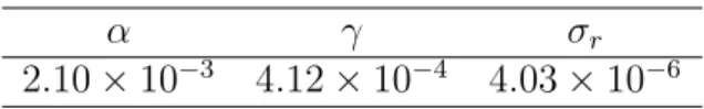
𝛼 𝛾 𝜎r
2.10×10⁻³
4.12×10⁻⁴
4.03×10⁻⁶
Table 5.1: Estimated parameters for the short rate model: long term mean γ, mean reversion speedα and short rate volatility σr.
1The One-day Interbank Deposit Futures Contract is a futures contract whose underlying asset is
the interest rate up to the contract’s expiration date, for this purpose defined as the capitalized daily Interbank Deposit (ID) rates verified on the period between the actual trading day and the last trading day. The ID futures contract are quoted in effective interest rates per annum, based on 252 business days convention, and its expiration date is always the first business day of the month of maturity.
2The first difference represents the absolute changes in the value of the short rate and is simply given
Figure 5.2 shows the generated tunnel of scenarios 3 for the annualized short rate for a
period of 3 years starting in January 2015, for 10.000 scenarios. It is possible to note the mean reversion behavior of the Vasicek model, suggesting an annualized long term short rate of 10% approximately.
Figure 5.2: Scenarios for the annualized short rate of the Brazilian interest rate.
5.1.2 Stock Prices
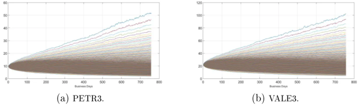
To implement the model for the stock prices defined in 4.14 it was necessary to estimate the parameters 𝜇 and 𝜎S, which accounts for the drift (the long term expected return)
and the volatility of the return on the stocks. To estimate those parameters, we first analyzed the historical data for the ordinary stocks for PETROBRAS S.A. (PETR3 ON) and VALE S.A. (VALE3 ON), which consisted in the series of the historical daily prices (adjusted close prices4) traded in the BM&F Bovespa stock exchange. Preferred stocks
may as well be used as underlying stocks of a stock swap, it its important that dividend payments should be incorporated into the price.
We analyzed the period from January 2006 to December 2014, as can be seen in figures
5.3 and 5.4 below for both counterparties:
(a) PETR3 prices. (b) PETR3 log-returns.
Figure 5.3: Historical data for the daily values of price and log-return for PETR3 (Petrobras ON) from January 2006 to December 2014.
3Instead of showing all the scenarios, in order to the make the analysis easier and clearer all the
tunnels presented in this work contain 200 percentiles for each date.
4Price adjusted to incorporate dividend payments, stock splits and any other changes in the value of