REAd | Porto Alegre – Vol. 24 – Nº 2 – Maio-Agosto 2018 – p. 218-229
WORLD FINANCIAL RELATIONS: UNDERSTANDING THE CREDIT
DERIVATIVE SWAPS (CDS) DEPENDENCE STRUCTURE
1Fernanda Maria Müller2 Marcelo Brutti Righi3 Anderson Luis Walker Amorin4
http://dx.doi.org/10.1590/1413-2311.200.78321
ABSTRACT
This study investigates the copula model that best fit to model the dependence structure of
Credit Derivative Swaps (CDS) spreads. For the analysis, we consider daily data from the
period of January 1, 2009 to December 31, 2014. Regarding the models, we considered Vine
copulas and Hierarchical Archimedean copulas, and different families of copulas. Our results
indicate that C-Vine copulas, as well Student t family, demonstrated better performance, according to the criteria used to get the dependence structure. The best fit of the dependence
structure can avoid the model risk, from the use of an incorrect model.
Keywords: Credit Derivative Swaps. Model risk. Vine Copulas.
1 Recebido em 27/11/2017, aprovado em 31/05/2018.
REAd | Porto Alegre – Vol. 23 – Nº 3 – Setembro / Dezembro 2017 – p. 218-229
219 RELACIONES FINANCIERAS INTERNACIONALES: ENTENDIENDO LA
ESTRUCTURA DE DEPENDENCIA DE LOS CREDIT DERIVATIVE SWAPS (CDS)
RESUMEN
Este estudio investiga el modelo copula que mejor modela la estructura de dependencia de
Credit Derivative Swaps (CDS) spreads. Para el análisis se consideraron datos diarios del período comprendido entre el 1 de enero de 2009 y el 21 de diciembre de 2014. Los modelos
considerados fueron las Copulas Vine y las Copulas Arquimedianas, con diferentes familias de
copulas. Nuestros resultados indican que las copulas C-Vine, así como la familia t Student, demostró mejor desempeño, de acuerdo con los criterios utilizados, para obtener la estructura
de dependencia. El mejor ajuste de la estructura de dependencia puede evitar el riesgo del
modelo, debido al uso de un modelo inapropiado.
Palabras clave:Credit Derivative Swaps. Riesgo del modelo. Copulas Vine.
RELAÇÕES FINANCEIRAS INTERNACIONAIS: ENTENDENDO A ESTRUTURA DE DEPENDÊNCIA DOS CREDIT DERIVATIVE SWAPS (CDS)
RESUMO
Esse estudo investiga o modelo cópula que melhor modela a estrutura de dependência de Credit
Derivative Swaps (CDS) spreads. Para a análise foram considerados dados diários do período de 01 de Janeiro de 2009 a 21 de Dezembro de 2014. Os modelos considerados foram as
Cópulas Vine e as Cópulas Arquimedianas, com diferentes famílias de cópulas. Nossos
resultados indicam que as cópulas C-Vine, bem como a família t Student, demonstrou melhor performance, de acordo com os critérios utilizados, para obter a estrutura de dependência. O
melhor ajuste da estrutura de dependência pode evitar o risco do modelo, decorrente do uso de
um modelo inapropriado.
REAd | Porto Alegre – Vol. 23 – Nº 3 – Setembro / Dezembro 2017 – p. 218-229
220 INTRODUCTION
Credit derivative swaps (CDS) have become a key innovation in the credit risk market
in the last few years, mainly because they are a versatile and adjustable financial instrument
that splits the credit exposure of financial products between two or more parties (ALNASSAR
et al., 2014). Coudert and Gex (2010) explain that the functionality of a CDS is simple, and that there are three parties involved: the credit buyer (CB), the credit seller (CS), and the
reference company (RC). CB therefore buys a CDS from CS against the default risk of RC. CS
guarantees to CB that he will receive a sum that compensates CB for his loss in the case of an
RC default. To do this, CS receives a percentage of the face value of the debt from CB for the
period of the contract or until RC defaults.
This simplicity and adjustability, along with the efficiency with which the swap acts as
a protection tool for financial players, creates a huge market for CDS (ABID; NAIFAR, 2006).
In this sense counterpart credit risk is one of the most important drivers of financial markets
(ARORA et al., 2012). Because of their importance, these derivative instruments have received attention from regulators, practitioners and researchers.
Correctly modeling the dependence structure of a CDS is important for risk managers
in order to set trading limits, for traders in order to hedge the market risk of their credit
positions, and for pricing credit derivatives (FEI et al., 2013). Financial assets usually present asymmetry, non-linear dependence, non-normality, and other stylized facts commonly reported
in the financial literature. The use of flexible models to deal with these characteristics will help
reduce problems arising from the model risk.5
Empirical studies on the insurance sector CDS indices have focused on analyzing the
dependence of these financial instruments using copulas. Abid and Naifar (2006) applied a
copula procedure on CDS from Japanese companies. Chen et al. (2011), who studied the
dependence among South American countries during the Argentinian debt crisis in 2001, used
a copula approach. Tamakoshi and Hamori (2014) investigated the dependence structure of the
CDS indices of the insurance sector in the United States, the European Union, and the United
Kingdom. In Gaiduchevici (2015) and Christoffersen et al. (2016) other uses of the copula
approach are identified.
Copulas provide a general approach to measuring dependence among groups of random
variables; in addition, this approach makes no assumptions about the distribution of returns. In
5 Model risk is related to sources of uncertainty caused by statistical models, such as model choice and the
REAd | Porto Alegre – Vol. 23 – Nº 3 – Setembro / Dezembro 2017 – p. 218-229
221 practical applications, the problem is to identify the correct copula to use for modeling the data.
For the bivariate case, there are various investigations. However, for multivariate cases, the
choice of adequate families is rather limited. An alternative is to use Vine copulas. Vines are a
flexible model for describing multivariate copulas using bivariate copulas (KUROWICKA;
COOKE, 2006). These constructions decompose a multivariate probability density into
bivariate copulas, where each copula can be chosen independently from the others, which
results in increased flexibility for modeling the dependence. Another possibility for modeling
multivariate dependence through copulas is the Hierarchical Archimedean method.
In this study, we investigate by means of copulas, the dependence structure of the CDS
spreads of 20 countries, using daily data from January 1, 2009 to December 31, 2014, which
corresponds to 1,565 observations. To reduce model risk resulting from the misspecification of
the copula, we carried out an exhaustive investigation to identify which copula models were
more appropriate for capturing the international dependence structure of CDS spreads, as well
as which model best adjusted the marginal distribution. In this work, we considered Vine
copulas and Hierarchical Archimedean copulas, and different families of copulas.
We believe that this study makes two primary contributions to the above strand of the
literature. First, it contributes to the identification of the copula model that reduces the model
risk of the dependence structure of CDS spreads. Appropriate dependence techniques are of
paramount importance in finance, since they are used as input into expensive decisions. On the
other hand, our results on the dependence structure are important for regulators wishing to
model the regulatory framework of the insurance sector.
1 COPULAS
To facilitate the presentation of the copula structure, we focus here on the bivariate case.
A function 𝐶 ∶ [0,1]2 → [0,1] is a copula for the cases in which 0≤ x ≤ 1, and x1 ≤ x2, 𝑦1 ≤ 𝑦2, (x1, 𝑦1), (x2, 𝑦2) ∈ [0,1]2. This function fulfils the following properties:
𝐶(x, 1) = 𝐶(1, x) = x, 𝐶(x, 0) = 𝐶(0, x) = 0, (1) 𝐶(x2, 𝑦2) − 𝐶(x2, 𝑦1) − 𝐶(x1, 𝑦2) + 𝐶(x1, 𝑦1) ≥ 0. (2)
The first property refers to the uniformity of the margins, and the second, the n
-increasing property, represents the fact that 𝑃(x1 ≤ X ≤ x2, y1 ≤ Y ≤ y2 ) ≥ 0 for (X, Y) with
REAd | Porto Alegre – Vol. 23 – Nº 3 – Setembro / Dezembro 2017 – p. 218-229
222 i) Given a copula C, and univariate distribution functions 𝐹1 and 𝐹2, a distribution
F, withmarginal distributions 𝐹1 and 𝐹2, can be represented by:
𝐹(x, y) = 𝐶(𝐹1(x), 𝐹2(𝑦)), for (x, y) ∈ ℛ2. (3)
ii) Let C be a copula that satisfies (3) for a two-dimensional distribution function
F with marginal distributions 𝐹1 and 𝐹2. C is unique if 𝐹1 and 𝐹2 are continuous, for every (x, y) ∈ [0,1]2:
𝐶(x, y) = 𝐹(𝐹1−1(x), 𝐹2−1(y)), (4)
where 𝐹1−1(x) and 𝐹2−1(y) represent the inverse of the marginal distribution functions of 𝐹1 and 𝐹2, respectively.
To extend bivariate copulas to the multivariate case, a flexible and intuitive way is to
use Vine copulas. In the literature, C-Vines, R-Vines and D-Vines are proposed. For brevity,
we present here only the C-Vine copula. In this case, the dependence in relation to a particular
variable, the first root node, is modeled using bivariate copulas for each pair. In conformity
with the work of Brechmann and Schepsmeier (2013), a root node is generally selected in each
tree, and all pairwise dependencies, with respect to this node, are modeled conditioned on all
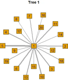
previous root nodes. The structure is similar to a star, as can be seen in Figure 1. The C-Vine
density, with root nodes 1, … , 𝑑, is represented by:
𝑓(x) = ∏ 𝑓𝑘 𝑑
𝑘=1
(x𝑘) ∗ ∏ ∏ 𝑐𝑖,𝑖+𝑗|1:(𝑖−1) 𝑑−𝑖
𝑗=1 𝑑−1
𝑖=1
(𝐹(x𝑖|x1, … , x𝑖−1), 𝐹(x𝑖+𝑗|x1, … , x𝑖−1)|𝜽𝑖,𝑖+𝑗|1:(𝑖−1)),
where 𝑓𝑘, 𝑘 = 1, … , 𝑑 represent the marginal densities and 𝑐𝑖,𝑖+𝑗|1:(𝑖−1) are the bivariate copula
densities with parameter(s) 𝜽𝑖,𝑖+𝑗|1:(𝑖−1).
2 EMPIRICAL ANALYSIS
We used daily data for the CDS spreads of Argentina, Belgium, Brazil, China, Costa
Rica, Croatia, France, Germany, Indonesia, Ireland, Italy, Jamaica, Korea, the Czech Republic,
Russia, South Africa, Spain, Thailand, Turkey, and the United Kingdom. These countries were
selected because they are representatives from different continents and present daily data
characterized by periods of turbulence and lulls. Our sample period was from January 1, 2009,
to December 31, 2014, which corresponds to 1,565 observations. We used log - returns of CDS
REAd | Porto Alegre – Vol. 23 – Nº 3 – Setembro / Dezembro 2017 – p. 218-229
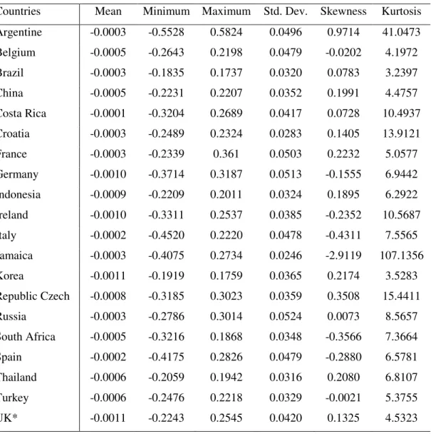
223 Table 1 - Descriptive statistics of the log-returns of CDS spreads, from January 2009 to
December 2014
Countries Mean Minimum Maximum Std. Dev. Skewness Kurtosis Argentine -0.0003 -0.5528 0.5824 0.0496 0.9714 41.0473 Belgium -0.0005 -0.2643 0.2198 0.0479 -0.0202 4.1972 Brazil -0.0003 -0.1835 0.1737 0.0320 0.0783 3.2397 China -0.0005 -0.2231 0.2207 0.0352 0.1991 4.4757 Costa Rica -0.0001 -0.3204 0.2689 0.0417 0.0728 10.4937 Croatia -0.0003 -0.2489 0.2324 0.0283 0.1405 13.9121 France -0.0003 -0.2339 0.361 0.0503 0.2232 5.0577 Germany -0.0010 -0.3714 0.3187 0.0513 -0.1555 6.9442 Indonesia -0.0009 -0.2209 0.2011 0.0324 0.1895 6.2922 Ireland -0.0010 -0.3311 0.2537 0.0385 -0.2352 10.5687 Italy -0.0002 -0.4520 0.2220 0.0478 -0.4311 7.5565 Jamaica -0.0003 -0.4075 0.2734 0.0246 -2.9119 107.1356 Korea -0.0011 -0.1919 0.1759 0.0365 0.2174 3.5283 Republic Czech -0.0008 -0.3185 0.3023 0.0359 0.3508 15.4411 Russia -0.0003 -0.2786 0.3014 0.0524 0.0073 8.5657 South Africa -0.0005 -0.3216 0.1868 0.0348 -0.3566 7.3664 Spain -0.0002 -0.4175 0.2826 0.0479 -0.2880 6.5781 Thailand -0.0006 -0.2059 0.1942 0.0316 0.2080 6.8107 Turkey -0.0006 -0.2476 0.2218 0.0329 -0.0021 5.3755 UK* -0.0011 -0.2243 0.2545 0.0420 0.1325 4.5323
Source: prepared by authors. * United Kingdom
Table 1 reports the descriptive statistics of the log-returns of the CDS spreads. Jamaica
presented the lowest standard deviation (Std. Dev.), while the CDS spreads for Russia showed
the highest standard deviation. In general, skewness values indicate which log-returns are
skewed. The series also showed excess kurtosis (they have fat tails), which is common behavior
for financial data. The kurtosis value for Jamaica (107.1356) stands out among the results.
In the first step, we estimated the conditional means and variances of the log- returns of
the CDS spreads. The Ljung-Box test indicated that there were significant autocorrelations in
the series. The conditional mean was adjusted by AR(1) (first-order autoregression)
REAd | Porto Alegre – Vol. 23 – Nº 3 – Setembro / Dezembro 2017 – p. 218-229
224 heteroscedasticity in the residuals of the AR models using the Ljung–Box test applied to the
squared standardized residuals and the Lagrange multiplier (LM) test applied to the
standardized residuals. The values for these tests indicated the presence of significant
conditional heteroscedasticity. In order to model the volatility of the CDS spreads we used
GARCH (Generalized Autoregressive Conditional Heteroskedasticity) models. Conditional
volatility was estimated using the GARCH, the exponential GARCH (EGARCH) and the
GJR-GARCH (Glosten-Jagannathan-Runkle GJR-GARCH) models. The probability distributions
considered were as follows: normal distribution, generalized error distribution (GED), Student
t distribution and asymmetric Student t distribution. To compare the fitted models, we analyzed the results using the Akaike information criterion (AIC), the Bayesian information criterion
(BIC) and the Hannan–Quinn information criterion (HQIC). Finally, to check the adequacy of
the fitted models we conducted an analysis of the residuals.6
Our results suggested that the EGARCH model using a generalized error distribution
presented the best results according to the AIC, BIC and HQIC. In this way, for the marginal
we estimated the AR(1)-EGARCH(1,1), with generalized error distribution. These results are
omitted for brevity reasons. The structure of the AR(1)-EGARCH(1,1) model is given by: 𝑟𝑖,𝑡 = 𝜙0+ 𝜙1,𝑡𝑟𝑖,𝑡−1+ 𝜀𝑖,𝑡,
𝜀𝑖,𝑡 = 𝜎𝑖,𝑡𝑧𝑖,𝑡, 𝑧𝑖,𝑡 ~𝑖. 𝑖. 𝑑. 𝐹(0,1),
ln(𝜎𝑖,𝑡2) = 𝜔 + 𝛼1𝑔(𝜀𝑖,𝑡) + 𝛽1ln(𝜎𝑖,𝑡−12 ), (5)
where, for asset i in period t, 𝑟𝑖,𝑡 is the log-return of the CDS spreads, 𝜎𝑖,𝑡2 is the conditional
variance, 𝜙0, 𝜙1, 𝜔, 𝛼1 and 𝛽1 are parameters, 𝜀𝑖,𝑡 is the innovation in expectation and 𝑧𝑖,𝑡 is a
white noise process with distribution F. 𝑔(. ) can be written as 𝑔(𝜀𝑖,𝑡) = 𝜃𝜀𝑖,𝑡+ 𝛾[|𝜀𝑖,𝑡| −
𝐸(|𝜀𝑖,𝑡|)], where 𝜃 and 𝛾 are real constants. We estimated the models using quasi-maximum
likelihood. The adjusted models exhibited a good adjustment to the data. The LM test and the
Ljung–Box test applied to the squared standardized residuals indicated the adequacy of our
models. Besides, the coefficients of the AR(1)-EGARCH(1,1) models were significant. After
isolating the marginal behavior, it was possible to conduct a joint analysis free of this marginal
influence. We used the residuals series 𝒛 = {𝑧𝑖,𝑡} and transformed it into pseudo-observations
𝒖 = {𝑢} ∈ [0,1]𝑝 by inversing the GED distribution fitted to each of them, because of the
domain and image definition of the copula functions. With these pseudo-observations, we
REAd | Porto Alegre – Vol. 23 – Nº 3 – Setembro / Dezembro 2017 – p. 218-229
225 estimated the C-, D- and R-Vines.7 The input order for the countries in the models was the
decreasing order of the sum of the absolute Kendall’s Tau of a country with all the others. From that, we obtained the following identification order: [1] Italy, [2] Turkey, [3] South Africa, [4]
Russia, [5] Spain, [6] Belgium, [7] Brazil, [8] Croatia, [9] China, [10] Ireland, [11] France,
[12] Korea, [13] Germany, [14] Czech Republic, [15] Indonesia, [16] Thailand, [17] United
Kingdom, [18] Jamaica, [19] Argentina, and [20] Costa Rica.
We considered the following copula families: Normal, Student t, Gumbel, Frank, Clayton, Joe, BB1, BB7, and BB8. Concerning the estimation of the parameters, we considered
an ML estimation procedure that follows a stepwise approach. In the first step, ML estimates
separately the parameters in each relationship. The parameter estimations obtained in this first
step are known as sequential ML estimates. In the second step, the full log-likelihood function
is maximized using the sequential ML estimates as starting values, resulting in the so-called
joint ML estimates.
The number of estimated parameters was huge, since there were 19 trees in each
structure. To keep this paper brief, we have omitted the estimated parameters, but they are all
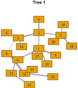
available upon request. Figures 1 to 3 exhibit plots of the main trees of the C-, D- and R-Vines,
respectively. From these plots we have a visual interpretation of how relationships occur. Of
course, there would be 18 more plots like this for each structure. We have also omitted these,
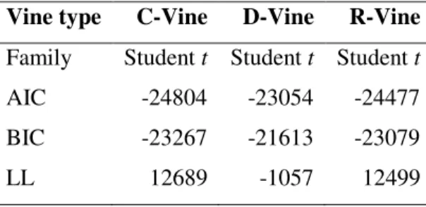
but they are available upon request. Table 2 shows the fitting results for the models.
Table 2 - Fitting statistics for the C-, D- and R-Vine estimated models
Vine type C-Vine D-Vine R-Vine
Family Student t Student t Student t AIC -24804 -23054 -24477 BIC -23267 -21613 -23079 LL 12689 -1057 12499
Source: prepared by authors.
To examine which copula was the best fit for the data, we considered the following
criteria: AIC, BIC, and LL (log-likelihood).8 We observed that the Student t copula is the
7 We also considered other complex copula constructions, such the Hierarchical Archimedean type, but their
performance was much worse than those of the Vines. In higher dimensions, Archimedean copulas have shortcomings for modeling asymmetric and complex dependences structures. For brevity, the results are omitted.
REAd | Porto Alegre – Vol. 23 – Nº 3 – Setembro / Dezembro 2017 – p. 218-229
226 predominant one, as is quite usual for daily financial returns. Regarding CDS analyses using
copulas, Chen et al. (2008), Tamakoshi and Hamori (2014) and Creal and Tsay (2015) also
verified that Student t copula are preferred over competing models. Referring to the Vine type, we observed that, according to the values of AIC and BIC, the C-Vine structure had the best
fit. For the values of LL, we found that the best value was presented by the D-Vine copula
(-1057).
A knowledge of the dependence structure among CDS spreads across countries, which
shows goodness of fit, is important for investors and regulators, because dependence is an input
relevant to portfolio allocation and risk management decisions. The use of families and types
of Vine copulas that present a better adjustment allows the regulator or manager to reduce the
model risk inherent in the process of estimation of the dependence, and consequently to reduce
financial losses arising from the use of an incorrect copula.
Figure 1 – C-Vine tree plot
REAd | Porto Alegre – Vol. 23 – Nº 3 – Setembro / Dezembro 2017 – p. 218-229
227 Figure 2 – D-Vine tree plot
Source: prepared by authors.
Figure 3 – R-vine tree plot
REAd | Porto Alegre – Vol. 23 – Nº 3 – Setembro / Dezembro 2017 – p. 218-229
228 CONCLUSIONS
Understanding the dependence behavior of CDS spreads is important because of the
popularity and liquidity of these instruments in the credit markets. This study focused on
determining the copula model that presented the best fit to model dependence structure of CDS
spreads in the multivariate context. In the analysis, we considered 20 countries and daily data
for the period from January 1, 2009, to December 31, 2014. The copula model allowed us to
capture the nonlinear dependence structure that is usually identified in financial data. From the
descriptive analyses, we noticed the presence of stylized facts in the log-returns for CDS. Our
main results indicated that the C-Vine structure and the Student t copula family presented the better performance. Thus, this specification is the most appropriate for obtaining the
dependence structure of the data considered, and possibly reduces the model risk arising from
the use of the wrong model.
REFERENCES
ABID, N.; NAIFAR, F. A. N. Credit-default swap rates and equity volatility: a nonlinear
relationship. The Journal of Risk Finance,v. 7, n. 4, p. 348 – 371, 2006.
ALEXANDER, C.; SARABIA, J. M. Quantile uncertainty and value-at-risk model risk. Risk Analysis, v. 32, n. 8, p. 1293–1308, 2012.
ALNASSAR, W. I.; AL-SHAKRCHY, E.; ALMSAFIR, M.K. Credit derivatives: did they
exacerbate the 2007 global financial Crisis? AIG: case study. Procedia – Social and Behavioral Sciences, v. 109, p. 026 – 1034, 2014.
ARORA, N.; GANDHI, P.; LONGSTAFF, F.A. Counterparty credit risk and the credit
default swap market. Journal of Financial Economics, v. 103, n. 2, p. 280-293, 2012.
BRECHMANN, E.C.; SCHEPSMEIER, U. Modeling dependence with C-and D-vine
copulas: the R-package CDVine. Journal of Statistical Software, v. 52, n. 3, 1-27, 2013.
CHEN, Y.-H.; WANG, K.; TU, A. H. Default correlation at the sovereign level: evidence
from some Latin American markets. Applied Economics, v. 43, n. 11, p. 1399-1411, 2011.
CHEN, Y.-H.; TU, A. H.; WANG, K. Dependence structure between the credit default swap
return and the kurtosis of the equity return distribution: evidence from Japan. Journal of International Financial Markets, Institutions and Money, v. 18, n. 3, p. 259-271, 2008.
CHRISTOFFERSEN, P.; JACOBS, K.; JIN, X.; LANGLOIS, H. Dynamic dependence and
REAd | Porto Alegre – Vol. 23 – Nº 3 – Setembro / Dezembro 2017 – p. 218-229
229 COUDERT, V.; GEX, M. The credit default swap market and the settlement of large
defaults. International economics, v. 123, p. 91-120, 2010.
CREAL, D.D.; TSAY, R.S. High Dimensional dynamic stochastic copula models. Journal of Econometrics, v. 189, n. 2, p. 335 – 345, 2015.
FEI, F.; FUERTES, A.M.; KALOTYCHOU, E. Modeling dependence in CDS and equity
markets: dynamic copula with markov-switching. Working Paper, 2013.
GAIDUCHEVICI, G. Modeling sovereign risk interaction in emerging Europe. Economic Insights, n. 4, v. 2, p. 117-124, 2015.
KUROWICKA, D.; COOKE, R.M. Uncertainty analysis with high dimensional dependence modelling. John Wiley & Sons, Chichester, 2006.
SKLAR, A. Fonctions de Repartition á n Dimensions et leurs Marges. Publications de l'Institut de Statistique de l'Université de Paris, v. 8, p. 229-231, 1959.
TAMAKOSHI, G.; HAMORI, S. The conditional dependence structures of insurance sector
credit default swap indices. North American Journal of Economics and Finance, v. 30, n.