An overview of some historical Brazilian macroeconomic series and some open questions

~.

FUNDAÇÃO GETULIO VARGAS

SEMINÁRIOS DE PESQUISA

ECONÔMICA DA EPGE

An Overview of Some Historical Brazilian

Macroeconomic Series and Some Open

Questions

RUBENS PENHA CVSNE

(EPGE/FGV)

Data: 23/06/2005 (Quinta-feira)

An Overview of Some Historical Brazilian

Macroeconomic Series and Some Open

Questions*

Rubens Penha Cysne

t

June

23, 2005

Abstract

This paper presents an overview of the Brazilian macroeconomy by analyzing the evolution of some specific time series. The presentation is made through a sequence of graphs. Several remarkable histori-cal points and open questions come up in the data. These include, among others, the drop in output growth as of 1980, the clear shift from investments to government current expenditures which started in the beginning of the 80s, the notable way how money, prices and exchange rate correlate in an environment of permanently high inHa-tion, the historical coexistence of high rates of growth and high rates of inHation, as well as the drastic increase of the velocity of circu-lation of money between the 70s and the mid-90s. It is also shown that, although net external liabilities have increased substantially in current dollars after the Real Plan, its ratio with respect to exports in 2004 is practically the same as the one existing in 1986; and that residents in Brazil, in average, owed two more months of their final income (GNP) to abroad between 1995-2004 than they did between 1990 and 1994. Variance decompositions show that money has been important to explain prices, but not output (GDP).

*Work in Progresso Please do not cite or quote. Key Words: Brazilian Economy, Money, Prices, Output, Balance of Payments, Investments, Inflation. JEL Classifications: EO, GO, HO, Nl and OI.

tprofessor at the Graduate School of Economics of the Getulio Vargas Foundation and a Visiting Scholar at the Department of Economics of the University of Chicago. E mail: rpcysne@uchicago.edu.

'

:.;

1é

1 Introduction

This paper provides a bird's eye view of the Brazilian macroeconomy within different periods of time. The analyses are carried out through the graph-ical view of some specific time series. For each series, the period of time contemplated in the study coincides with the period in which the data is

digitally available in primary data bases1_{• The series go as far in the past}

as 1900, the first year for which there is an estimate of Brazilian GDP. Ali other series start in 1947 or !ater, due to the unavailability of ofl:icial data concerning previous periods. In some cases, the equivalent series for the U.S. is displayed for the purpose of comparison.

A second objective of the paper, besides summing up historie economic

information about Brazil, is raising some questions the answers of which are still open to economic research.

The paper proceeds as follows. Section II concentrates on the GDP

growth between 1900 and 2004, taking the U.S. as a benchmark. Sections

I l i and IV deal, respectively, with capital formation and pu blic finance.

Section V concentrates on money and prices and section V I on the foreign

sector (balance of payments) and exchange rates. Section V I I points out

some open macroeconomic questions. Finally, section VIII concludes.

2

GDP

Figure 1 presents the evolution of the Brazilian and of the U.S. real GDP

(Gross Domestic Product) between 1900 and 2004. In both graphs, for the

purpose of comparison, the y-axis has been arbitrarily normalized to start

at one. Because I am using logarithmic data, rates of growth can be easily

inferred by taking the difference between y-coordinates at different points of time.

1 _{I call primary data bases those provided by the federal government (including Banco}

Central do Brasil, Tesouro Nacional, Ministério da Fazenda, MiniStério do Planejamento,

Fundação IBGE and IPEA) and the Fundação Getulio Vargas. The respective sources of

each time series used in the work are presenteei in Appendix.

I

i!í'h"'

,,----Brazilian Real GDP: 1900-2004 U.S. Real GDP: 1900-2004

6.5 6.5

6

+

-+

- I 6

+

-+

1 I

-5.5 -1-

-+

-1 5.5 -1-

-+

1 1

-5 -L _J_ -1 1 - 5 -L _J_ 1 1

-4.5 j__ _]_ _I I _ 4.5 j__ _]_ _I

.§' ₄ _I _I

_-

I

_-

.§' ₄ _I _I

_-

I

c.. _{I I I} c.. _{I _I I}

Cl _3.5 Cl _3.5

""

- -

""

1i! I

_&!

"'

3

-

-

3

2.5

-

-I 2.5

-2

-I

-

-

-

I

-1.5 _{- I -~-} 1.5

-~-1 1

1900 1920 1940 1960 1980 2000 1 900 1920 1940 1960 1980 2000

Year Year

Figure 1

Regarding the Brazilian economy, one point . that comes up in the left pane! of Figure 1 is the break in the historical rate of GDP growth in the beginning ofthe eighties. Average growth was 5.68% between 1900 and 1980 andjust 2.11% between 1980 and 2004, totalling 4.85% per year in the whole period. This can be inferred from the left pane! of Figure 1 by drawing a straight line connecting the data in 1900 an 1980, extrapolating it to 2004, and subtracting its y-coordinate in 2004 from the y-coordinate of the original data.

If the Brazilian economy had kept its 1900- 1980 historical growth as of 1980, the GDP and the per-capital income in 2004 would have been around 2.28 times the one which actually prevailed. In Reais (Brazilian present monetary unit) of2004, thls would mean a per capita domestic in come around

R$ 23,014, instead of just R$ 10,094. In average dollars of 2004, U$ 7, 865.

3, instead of U$ 3, 449.82

.

Would it be the case that the growth decline in the 80s was somehow associated with a similar downturn of the industrialized economies?

The right pane! of Figure 1 presents the evolution of the United States GDP for the same period. Average growth for the United States reached

2_{The average sale values of the dollar in 2003, 2004 and from Jan 1 to June 02 of 2005}

;)ctween 1900 and 1980 and 3.14% between 1980 and 2004. Repeating the calculations mentioned above for Brazil, if the United States had grown as of 1980 at its 1900 -1980 rate, the ratio between projected real GDP and actual real GDP would have reached just 1.09 in 2004, in contrast to the ratio of 2.28 for Brazil. Assuming that the behavior of the remaining industrialized countries could be approximated by that of the U.S. economy, the answer to

the question posed in the preceding paragraph is clearly negative. It looks

like most of the Brazilian loss of GDP after the 80s is to be explained by its own economic policies, rather than by externaI factors.

The calculations mentioned so far pertain to a type sometimes found in

01' the Brazilian economy. Even though the numbers do point out in

the right direction, a more careful extrapolation provides different numbers. The figures inferences above are too dependent on the points in time in which they are taken (respectively, 1900, 1980 and 2004). Extrapolating the GDP of a certain economy at a certain point in time is not a good practice because at this time this economy could be in different positions

of its business cycle3. A way of dealing with this problem is estimating the

average rates of growth based on a least-squares approximation, rather than

on point estimates4

•

Figure 2 repeats Figure 1, this time adding an extrapolation to the 1981-2005 period based on a 1900 - 1980 least-squares fito

3 A secomd point is that the calculations are deterministic, and have not taken into

consideration the different shocks that can impact long-run leveIs of GDP. In this paper I shall not be concerned about this facto

4 A log-linear trend can be interpreted as a rough estimation of potential output, which

,

.

Brazilian Real GDP: 1900-80 Extrapol.

6.5 r , r , . . , ,

-, ,

, , .,

6 --- ..

·-1---····

T" ----

'i'-.-... 'i'--'

'/.~---5.5 --- - - --~ - - - --~ -- ---i- --- -- -~- r -- -~-

-, , . . /'

.

:g

4:

::::::r:::r:::T:M:::::F

i

3.:

···:·:["I;f:·L·J·::·:T·

:~ LI::~t::TJ::~:::l~

1900 1920 1940 1960 1980 2000 Year

Figure 2

- - -

-U.S. Real GDP: 1900-80 Extrapol.

6.5 r----,..----,----,----,---.---,

6 - - - .. -

-i ---.

'1- ----.. -1- ---.. --i- - -:-

--- I

1f ::: ·· ..

:.[].:E:J:·::T:

a. 4

---;--

---r-§ 3.5 ---:---:---:----

--:---:---i

3

---r---l---

i--:---I---+--:: :.' i--:---I---+--::: :,!: ... : ..

~:

':':.

t·: ":.]':: : ...

J:"

1 - - - -- -

+---+---+ ---+ ---

---4---1900 1920 1940 1960 1980 2000 Year

These alternative calculations indicate a "GDP loss" of just 52.08% for Brazil between 1980 and 2004, instead of the 128% reported before. The reason for such a discrepancy is that, as one can observe from the left panel of Figure 2, the output in 1980 was above the potential output determined by the log-linear trend used in the projections.

The change of procedure does not affect the number for the United States. Under the alternative methodology based on least-squares log-linear extrap-olation the "lost GDP" for the United States reads 9.06% (against 9.0% before).

A comparison between both graphs shows that Brazil has grown a way

more than the United States during the 20th century. Maybe a good example

of a catch-up of a latecomer.

3 Investments

;eJJt; li 41 .([Uilti 2

Brazil - Capital Formation as a Fraction of GOP

0.3r---~---_r---,_---r_----_.r_----_.---,

0.28

0.26

õ:

C\ 0.24

C)

::::..

§ 0.22

1ã E

af 0.2

~ _g.

0.18

u

0.16

0.14

-.L

,

T

+

_,

-

,

T

-+--.l

,

I

--i

-

_,

--,-

--1

I"

,

-+

0.12L---~---L---~--- __ L _ _ _ _ _ ~ _ _ _ _ _ _ _ L _ _ _ _ _ _ ~

1940 1950 1960 1970 1980 1990 2000 2010

Year

Figure 3

Capital formation increases till the end of the eighties. By this time, the large investment projects initiated under the military governments started to cease, and capital formation starts to decline.

The situation seems worse when one consider capital formation with 1980 prices, as displayed by Figure 4 (this time, as of 1970 only):

-Brazil - In\lestment as a Fraction of GDP, Calculated with 1980 Prices 0.26

I I I

0.24 _{- l - I}

-c::- "I I

o

S:2 0.22 -

-gf

c.:>

. .::

1-D....

0.2

<::> L .J.

DO

CJ)

I

:c.

.::

+

-t

o 0.18

1ã

-+

ê _{I I}

~

=[ 0.16 T

-,

cu

u

0.14

-

-0.12

1970 1975

Year

Figure 4

This decrease of investments is certainly to be included among the explana-tions concerning the fall of GDP growth as of 1980.

4

Public Finance

At the same time in which capital formation started decreasing in the begin-ning of the 80s, public consumption, which includes mostly wage payments in the three administrative public leveIs (federal, state and local governments), started increasing. In twenty years, it practically doubled. Figure 5 shows this point quite clearly:

Brazil - Government Consumption as a Fraction of GDP

0.22r---r---,---,---.---.---.---~

0.2

ã:" 0.18

CI

(!)

~

"'o:: 0.16

o

a

E

:::::2 0.14

~

~ 0.12

0.1 I T I -L I I

-t

l

-I

--

-I

_ 1

1

-I 1-I l -I 1-J. I -t I I 0.08~---L---~~----~~----~---~---~---~

1940 1950 1960 1970 1980 1990 2000

Year

Figure 5

Taxes as a percentage of GDP, on the other hand, have kept their increasing trend as of 1990:

Brazil - Taxes as a Percentage of GDP

36

I I

34

+

_---I - l - _{I -}

-t-I I I I

32

+

--I 1-

-+

ã:" _I

I

CI

(!)

~ 30 -I-- -I -I-

--+

m

_{I I}

~

_-+-

-I---+

28

26 1- L

I I

24

1990 2000 2002

Year

Figure 6

2010

..

' , . " . : " ' : .">

Net public debt as a percentage of GDP, as shown in Figure 7, have increased steadily between 1996 and 2002, showing a small reversion between 2002 and the 2005:

Brazil - Net Public Debt as a Percentage of GDP

65r---,---r---,---.---.----~---._---,

60

55

6:'

g

50

~

:õ

~ 45

.g

:c

~ 40

ã) :z

35

30

I

-

I-1

1 1 1 1

-1- 1- 1 1

-- 1 -- -- 1 -- -- I

1 1 1

- 1 - - 1 - - I

25L---~----~----~~----~---L----~---~----~

1990 1992 1994 1996

Figure 7

1998

Year

2000 2002 2004

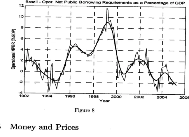
Another fiscal variable largely used in Brazil is the Operational Net Public Borrowing Requirements (NPBR). This variable is equal to the deficit cal-culated with real interests plus the inflation tax and encompasses not only the three public administrative leveIs but also state enterprises and public social security. When the inflation tax is negligible, the operational defict translates precisely the variation of the real value of the net indebtness of the government. Figure 8 shows the evolution of this variable between 1992 and 2005, in a 12-month moving sumo As usual, the red line translates the trend. The negative values presented as of 2003 are associated with the fall of the net indebtness shown in the preceding figure.

Brazil - Opero Net Public Borrowing Requriements as a Percentage of GDP

12~----~---~---~---r ______ ~ ______ ~ ____ ~

10

_--

-I I _I

s

₊

_-I

_+-

_-+

ã:' o

I C!>

~ 6

I

o:: tIl

-+-

_-+

a... ₄

:z

ãi c

.2

2

i!! _I

Q)

c.. O

l

-O

-2

-

--4

1992 1994 1996 1998 2000 2002 2004

Vear

Figure 8

5

Money

and

Prices

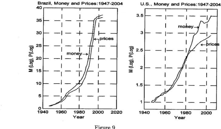
Figure 9 below shows the long-run relationship between money (M1) and

prices in Brazil (left panel) and in the United States (right panel).

The visual correlation (numerically, 0.994) in the Brazilian case is

remark-able. AE before, in both cases an arbitrary normalization is done in order to

have the y-axis starting at one. This is trivial for prices, which are

repre-sented by an indexo Regarding M1, the normalization implies redefining the

unit of account. In any case, what matters are the rates of growth implied by the differences of the y-coordinates at different points of time.

Brazil, Money and Prices:1947-2004

40 U.S., Money and Prices:1947-2004 35

30

10 5

I I

- I

+

I I

_I ~on.!-+

1-+-rPrices

1l

I -I

1-OL-_~L-_~ _ _ ~L-_~

1940 1960 1980 2000 2020 Year

Figure 9

3.5

3

1.5

1 1940

1 l

-I l -I

1-1960 1980 Year

In both cases, money grows faster than prices, which can be (tautolog-icaIly) read as a positive growth of the ratio between real GDP and the velocity of circulation of money. In the Brazilian case, between 1947 and 2004 the average growth rates of money, prices and real GDP were,' respec-tively, 87.0%, 84.0% and 5.1%, numbers which imply an average increase of M1 velocity at the rate of 3.39% a year.

It is clear from Figure 9, by the slope of the price line, how the

stabi-lization of inflation was successfully reached in 1994. It took democracy ten

years to deliver low inflation. It is still an open question how many additional

years it wiIl take to deliver a reasonable sustained growth of the per capita income.

Figure 10 shows the evolution of M1 as a fraction of the nominal GDP

and inflation.

- I I _I I

M1 as a Fraction of GDP and Inflation

3000 0.12 _T

_-

_-

_-r

_-

-~

-

-I 2500 0.'1

T -

-

I

-,

I ~ Inflalion 2000 0.08 -

-I

-

-

_I

>- c::

e:

_{1500 ~}

~ 0.06

-

-

_-

_-

<;::

.E

0.04

-

-

_-

_-

1000

0.02

-

-

.L

_-

-

_-

_-

500

O

O

1960 1970 1980 1990 2000 2010

Year

Figure 10

The ratio between Ml and nominal GDP has fallen steadily from 12.7

%

in 1971 (because infiation increased and also because of the financiaI innova-tions introduced at this time) to less than 0.1% in the early 90s. After 1994 it recovered steadily, reaching around 5.0% in 2004. With a money multi-plier around 1.47 (average between January of 2004 and April of 2005), this implies a ratio around 3.4 between the monetary base and nominal GDP.

6

Foreign Sector

• Extemal Savings

Figure 11 shows the evolution of the current account of the Brazilian

-..----Brazil - B.of P: Current Account, 1947-2004

X 104

2r---r---.---.---~----_.---,_----~

§ -2

o

~

c

~-3

::::J

(.)

I

-+

-+

I

...L

-4 I -4 I

-J

I

1

1

l

l -I

I

1I

-1

1

-l-L

1

4 L -____ - L _ _ _ _ _ _ L -_ _ _ _ ~ _ _ _ _ _ _ L _ _ _ _ _ ~ _ _ _ _ _ _ ~ _ _ _ _ ~

rs

1940 1950 1960 1980 1990 2000 2010

Year

Figure 11

Between 1947 and 2004, Brazil has saved to the rest of the world in only 9 years: 1950, 1964, 1965, 1984, 1988, 1989, 1992, 2003 and 2004. In

the remaining 49 years, Brazilian net externaI liabilities (which equaI net externaI debt plus n.et foreign direct investments5 _{in Brazil) have increased.}

The excess of internaI investments over domestic savings in BraziI has been particularly high from the seventies to before the mid-eighties and be-tween 1995 and 2002.

The highest current account deficit, both in millions of current dollars or in dollars of 1947, occurred in 1998 (U$ 33,416 and U$ 5,3708, respectiveIy). The record high untiI1996, in millions of 1947 dollars, happened in 1982 (U$ 4,0225) .

• Net ExternaI Liabilities

The historical variation of the net externalliabilities as of 1947 is shown in Figure 12 in current dollars, in 1947 dollars and as a ratio with respectto exports:

X 105 Brazil - Variation of Net Externai Liabilities 1947-2004 3.5 r-,----~---r_---_r----~r_---,_---_,7

3

,-~ .!!! C5 2.5 c t;: C )

--

,---.:::I 2 o::::: cu c ê _:::J

1.5

,-g

.Q

,

~

~ 1

,-w

10

:z 0.5

,

T

-,--,-

_,

,

T

-,-r

6

5

1

rs

O L-L-____ ~====~~==~

__

_L ______ ~ ______ L_ ____ ~o

1950 1960 1970

Fugure 12

1980 Year

1990 2000

Net externalliabilities (in Portuguese, Passivo Externo Líquido - call it D) have reached U$67, 516 +D46 millions in 1980, D46 standing for the initial value of this variable in millions of current dollars, in December 31, 1946. Between 1981 and 2002, additional U$ 224,189 millions have been added to these liabilities, making a total of U$ 291, 705 in the end of 2002. By subtracting the positive excess of the GNP (Gross National Product) over the internai absorption of goods and services in the years 2003 and 2004, one obtains the final figure for the net externaI liabilities existing at the end of 2004: U$ 275, 883+D46 millions.

The final number, of course, depends on the net externalliabilities ex-isting and the end of 1946. In current dollars, these can be considered to be negligible, in which case one obtains the final figure for the Brazilian net externaI liabilities in December of 2004 : U$ 275, 8836_.

In order to compare the absorption of externaI capitais between the 1973 - 1981 years (1973 standing for the year of the first oli crisis) and

6Data of the current account of the Balance of Payment between 1930 and 1947, for instance, can be obtained from the IBGE, "Estatísticas Históricas do Brasil. Rio de , Janeiro". By adding up all current account deficits between 1930 and 1946, one obtains a value of the net externalliabilities in the beginning of 1947 equal to U$ -1041.2 millions

+

D1930 · Here, D1930 stands for the net externalliabilities in the beginning of 1930. The

net externallliabilities at the end of 2004, therefore, can also be expressed as U$ 274,841.8 millions +D1930 •

the 1994 - 2002 period (1994 being the year in which the Real Plan was launched), it is appropriate that the figures above are reported in constant dollars. Using millions of dollars of 1947, the accumulated real-value cur-rent account deficit reads a total of U$ 23,895 in the years 1973 - 81 and U$ 30,031 in the years 1994 - 2002. In these terms, the eight years after the Real Plan have used 25.7% more externaI savings than the eight years after the first oil crisis (which includes the second oil crisis in 1979 and the upsurge of interest payments in the beginning of the eighties). Also in constant dollars, the period 1994 - 2004 responds for 43.0% of the total accumulation of net externalliabilities since 19477 •

Make X denote exports. The ratio D/X gives one possible measure of the exposure associated with externalliabilities. In the Brazilian case, the historical peak of this ratio occurred in 1999. The value attained at this time, though, v;:as practically equal to the one existing at the end of 1986. At the end of 1999 a payout of net externalliabilities required 59.1 months of the export revenues. At the end of 1986, 57.8 months.

Another interesting point. At the end of 2004, 34.3 months of exports were needed to liquidate the net externaI liabilities. This number is just slightly superior to the average one (32.0 months) existing in the three years before the Real Plan was launched (1992 - 1994). Under this criterion, therefore, there has been no increase of the externaI exposure after the Real. An alternative indicator of externaI indebtness uses a ratio with respect

to the Gross National Product (GNP), rather than exports. Although one

does not pay externaI liabilities with G N P, this is the right criterion to use when one is concerned with the average effort of a resident in Brazil to pay the country's net externaI liabilities. Under this alternative criterion, the numbers are as follows.

Between 1990 and 1994, under the average price of the dollar at that time, net externaI liabilities were worth 2.9 months of GN P. Using data of the years 1995 - 2004, one obtains 4.9 months, a 69% (or 2-month) expansion. The increase seems pretty modest, when compared with the high leveIs of consumption enjoyed after the Real and with the achievement of having stabilized inflation.

• Exchange Rates

Figure 13 shows the evolution of exchange rates since 1947. The left

70f course, thefigure is higher (62.40%) when the calculation is performed in cuirent

graph adds prices to the plot, whereas the right one adds both prices and money:

E. R. and Money (M1) 40~----r---~----~ __ ~ 35 30 I --I I I

+

I

~ 25

I

I--' C

o...

li

20 --I

I I --I

c:::

ui 15

1--

I--110

15

I:)L..---.L-____ L-. _ _ _ L-. _ _ - - J

1940 1960 1980 2000 2020 Year

Figure 13

Nominal E. R. and Prices 4 0 . - - - . - - - . -____ . -__ ~

35 30 I --I I

+

~ 25

I -I

' C

a..

li

20 --I

I I --I

I--c:::

ui 15 _l

-

I--10 5

O L - - - - . L -_ _ _ L-. _ _ _ _ .L-_ _ - - J

1940 1960 1980 2000 2020 Year

As it happened with money and prices, figure 13 shows a remarkable corre-lation between exchange rate and money or prices.

• Real Exchange Rates and Commercial Balance

,

..

5000 Brazil - Commercial Balance and Real Exch. Rate

I ~IReal E. R.

4000 _{- I}

_+-

₊

₊

_-

_-

_l

-I I I I

'"

c:

o

-I _-I-

₊

~ 3000

_-

--

I

=> >:

:c 2000

-+-1: _o

;:§..

C>..

f-E 1000

-;-C>..

><

w

O _~..2.o~aL

-1000

1983 1986 1990 1994 1999 2005

Year

Figure 14

On the right axis one reads the real exchange rate. An important point

to be noticed is the delay between changes of value of the real exchange rate and their effects over the commercial balance.

This point is particularly important in the present moment, in which the combination of high interest rates with flexible exchange rates has lead to a much lower price of the dollar than the one which happened last year. Following the trends shown in figure 14, this is supposed to generate a fall of the commercial balances in the near future, a fact that has to be taken into consideration by the present managers of economic policy.

7 Variance Decompositions

Figures 15 a, b and c provide a variance decomposition for a V AR with log

of GDP, log of prices and log of Ml, in this order, with a four year-horizon

and using, respectively, 8, 4 and Ilags:

percentages of ~orecast Error in ROWS Explained by columns

y p m Y 79.96339 1. 57973 3.13367 P 2.66195 17.84278 8.74950 m 17.37466 80.57749 88.11683 150 140 130

120 >< -8 _c:

110

-;-fd

100

a::

.c:

.g

90 w

80

70

Per cent ages Df FDrecast Errar in RDWS Explained by calumns

y p m

y 95.78056 0.09369 4.12575

P 1. 24292 2.08408 96.67300

m 3.09465 0.75747 96.14788

Figure 15b, Variance Decomposition, VAR with 4 Lags

percentages af Farecast Errar in Raws Explained by calumns

y p m

y 96.26412

1. 21839 0.63509

P 0.47568 5.50960 5.06999

m 3.26020 93.27201 94.29492

Figure 15c, Variace Decomposition, VAR with 1 Lag

It is interesting to see that money explains a fraction no greater than 18%

of the variance of the GDP and no lower than around 80% of the variance of prices. This order of magnitude is reasonably robust to changes in the forecast borizon. Prices, on the other hand, explain less than 6% of the variance of money.

8

Some Open Questions

Some points observed above require further investigations.

First, the drop in output growth as of 1980 (Figures 1 and 2). After 15 years, the country has not been able to resume its 1900 -1980 historical rate of growth. Does it translate a temporary downturn or a structural change in

the Brazilian pattern of growth8_?

..

between 1980 and 1984 (e.g., the Lei da Informatica in 1984); heterodox

sta-bilization plans carried out between 1986 and 19919_{, which failed miserably}

and cluttered the economy; the difficulties to economic policy making

intro-duced by the Constitution of 198810 etc. The main point here, though, is not

pointing to this or that reason, but understanding if a fast recovery to the old rates of real output growth is technically feasible or not, and if positive, under which policies and/or circumstances.

The precedent analysis (Figures 3, 5 and 6) suggests that a shift from public current expenditures to the formation of capital is one of the important ingredients, if a return to the old growth rates is to be achieved.

Second, as Friedman (1968, p. 1) points out, some economists regard rapid growth and absence of price stability as incompatible. Brazil, however, as one can notice from Figures 1 and 9, provides a clear counter-example to

this claiml l

. This is a country in which monetary policy has certainly not

fulfilled its function (in the words of Friedman) of "preventing itself of being a major source of economic disturbance." Notwithstanding, between 1947 and 2004, to restrict to the time period in which monetary data is available, average yearly GDP growth reached 5.1% , whereas inflation presented a

yearly average of 85.9%. It is therefore an open question how those who, see

inflation and rapid growth as incompatible respond to this data. ' ,

Third, Figure 10 suggests that the remarkable increase of the velocity of circulation of money in the beginning of the seventies seems to have gone be-yond the one which could be explained based only on the increase of inflation and nominal interest rates. In other words, there was a autonomous shift of the money demand as of this date. This fact has been documented initially

by Cysne (1984 and 1985) and later by Rossi (1986, 2000). It remains an

open question to detail how this shift in money demand has been related to the issuance of the ORTNs (Obrigações Reajustáveis do Tesouro Nacional), as of the mid sixties, of the LTNs (Letras do Tesouro Nacional), as of the early seventies, and also to the repurchase agreements, which granted much more liquidity to the public debt as of this date.

Fourth, a point of a more historical nature (or methodological, ir the

9The Cruzado Plan in February in 1986, the Cruzadinho in July of 1986 (basically, a fiscal package), the Bresser Plan ofmid-1987, Plano Verão (Summer Plán) in 1989; Plano Collor I in 1990 and Plano Collor II in 1991.

lOThe Constitution of 1988 transferred Federal revenues to states and municipalities without reciprocities regarding the provision of public services. It also increased labor costs and the earmarking of revenues, potentially shifiting future fiscal adjustments from healthy decreases of current expenses into unhealthy increases of ineflicient taxation.

original series is to be questioned) between 1929 and 1933 the American GDP decreased 26.6%. Brazilian GDP, on the other hand, shows a contraction of just 5.23% between 1929 and 1931 and, somewhat surprisingly, an increase of 7.73% between 1929 and 1933. Given the high dependence of the Brazilian economy on its export markets at that time, how can one account for this high GDP growth between 1929 and 1933?

9

Conclusions

This paper has aimed at presenting an overview of the Brazilian Economy 'covering the period 1900-2004. Besides the descriptive purpose of putting together large amounts of data in an easily recognizable way, some empirical points have been remarked, whereas others have been suggested as demand-ing empirical research.

Some of the subjects raised here, such as the proper identification of the potential output of the economy; the lag between real exchange rate and its effect on the commercial balances; the increase of public current expenditures and the concomitant falI of investments, have practical effects in the present management of macroeconomic policies. Others are of a more historical nature.

The main conclusions of the overall analysis have already been summa-rized in the introduction of the work.

References

[1] Cysne, R. P. (1984): "Macroeconomic Policy in Brazil: 1964-66 x 1980-84" . Doctoral Dissertation, Graduate School of Econornics, Getulio

Var-gas Foundation. Published by Losango SA, Rio de Janeiro.

[2] Cysne, R.P., (1985), Moeda Indexada, Revista Brasileira de Economia 39, no. 1, Jan.jMar.,57-74.

[3] Friedman, M. (1968). The Role of Monetary Policy. The American Eco-nomÍC: Review, LVIII, n. 1.

[4] Braun, Steven (1990). "Estimation of Current-Quarter Gross National

pu

•

--- -l

I

[6] Clark, Peter K. (1982). "Okun's Law and Potential GNP." Board of Governors of the Federal Reserve System, October.

[7] Estrella Arturo, and Frederic Mishkin (1999). "Rethinking the Role of NAIRU in Monetary Policy: Implications of Model Formulation and Uncertainty." In Monetary Policy Rules, edited by J. B. Taylor, pp. 405-430. Chicago: University of Chicago.

[8] Haddad, Claudio (1978). "Crescimento do produto real no Brasil, 1900-1947". Rio de Janeiro: Fundação Getúlio Vargas.

[9] Okun, Arthur (1962). "Potential Output: Its Measurement and Sig-nificance." In American Statistical Association 1962 Proceedings of the Business and Economic Section. Washington,D.C.: American Statistical Association.

[10] Rossi, J.W. (1986). "The Demand for Money in Brazil Revisited", TDI- . 96 (IPEA/INPES, Rio de Janeiro).

[11]

Rossi, J.W. (2000). "The Demand for Money in Brazil: \Vhat Happened in the 1980s?" Journal of Development Economics 31 (1989) 357-367. North Holland

[12] Taylor, J. B. (1993). "Discretion Versus Policy Rules in Practice". Carnegie-Rochester Conference on Public Policy 39: 195-294 .

Appendix - Sources of the Data

Real GDP, Brazil - Original Source, Haddad (1978) -from 1900 to 1947-, FGV and IBGE. Secondary Source, Data Bank of the Getulio Vargas Foun-dation.

Real GDP, U.S. - Federal Reserve Bank of St Louis (FRED)

Money - Original Source Central Bank of Brazil. Secondary Source Data Bank of the Getulio Vargas Foundation.

Prices - IGP-DI, Source, Getulio Vargas Foundation.

Current Account Deficit of the Balance of Payments - Central Bank of Brazil .

. Exports - Central Bank of Brazil.

GDP-GNP = Net income transferred to Abroad - Central Bank of Brazil.

GDP in current dollars - Central Bank of Brazil

Nominal Exchange Rate -: Data Bank of the Getulio Vargás Fouildation

FUNDAÇÃO GETULIO VARGAS

BIBLIOTECA

ESTE VOLUME DEVE SER DEVOLVIDO A BIBLIOTECA NA ÚLTIMA DATA MARCADA

BIBLIOTECA MARIO HENRIQUE SIMONSEN

FUNDAÇÃO GETÚLIO V/\RGAS