Fertility and the value of Life

April29, 2003

Fertility and the Value of Life

Abstract

The value of life methodology has been recently applied to a wide range of contexts as a means to evaluate welfare gains attributable to mortality reductions and health improvements. Yet, it suffers from an important methodological drawback: it does not incorporate into the analysis child mortality, individuals’ decisions regarding fertility, and their altruism towards offspring. Two interrelated dimensions of fertility choice are potentially essential in evaluating life expectancy and health related gains. First, child mortality rates can be very important in determining welfare in a context where individuals choose the number of children they have. Second, if altruism motivates fertility, life expectancy gains at any point in life have a twofold effect: they directly increase utility via increased survival probabilities, and they increase utility via increased welfare of the offspring. We develop a manageable way to deal with value of life valuations when fertility choices are endogenous and individuals are altruistic towards their offspring. We use the methodology developed in the paper to value the reductions in mortality rates experienced by the US between 1965 and 1995. The calculations show that, with a very conservative set of parameters, altruism and fertility can easily double the value of mortality reductions for a young adult, when compared to results obtained using the traditional value of life methodology.

Keywords: value of life, mortality, fertility, survival rates

JEL Classification: J17, J13, I10

Javier A. Birchenall

Department of Economics, University of Chicago, 5107 S. Blackstone Ave. #1007, Chicago IL 60615 e-mail: jabirche@uchicago.edu.

and

Rodrigo R. Soares

Department of Economics, University of Maryland, 3105 Tydings Hall, College Park, MD 20742; and Graduate School of Economics, Get´ulio Vargas Foundation, Rio de Janeiro, Brazil

e-mail: soares@econ.umd.edu

∗_{We benefited from comments from Roger Betancourt, Kevin Frick, Esteban Rossi-Hansberg, Seth Sanders, and}

“In many parts of the Essay I have dwelt much on the advantage of rearing the requisite population of any country from the smallest number of births. I have stated expressly, that a decrease of mortality at all ages is what we ought chiefly to aim at; and as the best criterion of happiness and good government, instead of the largeness of the proportion of births, which was the usual mode of judging, I have proposed the smallness of the proportion dying under the age of puberty.”

Thomas R. Malthus (1826)

1

Introduction

This paper incorporates fertility and altruism into the “value of life” approach. We develop a manageable way to deal with valuations of reductions in mortality rates when fertility choices are endogenous and individuals are altruistic towards their offspring. Our framework, designed to account for non-monetary aspects of welfare gains, falls on the tradition inaugurated by Schelling (1968), and extends previous techniques developed by Usher (1973), Arthur (1981), and Rosen (1988, 1994), among others.

Recently, the value of life methodology has been applied to a wide range of contexts as a means to evaluate welfare gains attributable to mortality reductions and health improvements. Nord-haus (1999), Murphy and Topel (2001), and Garrett (2001) applied this methodology to analyze different aspects of health related gains in welfare in the United States throughout the twentieth century. Becker, Philipson, and Soares (2003) applied an adapted version of this technique to evaluate the evolution of welfare inequality across countries, once improvements in life expectancy are accounted for.

welfare of the offspring.1

In the paper, we evaluate the welfare implications of mortality reductions in a setup where individuals choose the number of children they have and are altruistic towards their children. We show that, under these circumstances, the value of adult mortality changes can be decomposed into three factors: the consumption factor from the traditional value of life specification, originally derived by Rosen (1988); a fertility factor, which accounts for the welfare improvements related to the higher probability of having children; and an altruism factor, which accounts for the fact that the mortality reductions will also be enjoyed by all future generations. Additionally, our approach allows us to calculate an adult’s willingness to pay for reductions in child mortality. This willingness to pay will generally depend on the effect of child mortality on thefinal costs of child production, the uncertainty regarding the number of surviving children, and, again, on the fact that these gains will also be experienced by all future generations.

To illustrate the empirical relevance of fertility and altruism in the value of life problem, we apply our methodology to value the reductions in mortality rates experienced by the US between 1965 and 1995. The parameterization of the model poses a series of new questions regarding the calibration of some unusual parameters. We try to deal with these in the most reasonable way presently possible. The calculations show that, with a very conservative set of parameters, altruism and fertility can easily double the value of mortality reductions for a young adult, when compared to results obtained using the traditional value of life methodology.

Most of the issues discussed in the paper touch on the more general question of how to deal with children and future generations in the evaluation of specific policy interventions. Since the value of mortality risks is a completely forward looking measure, egoistic adults who survive child-hood place zero value on mortality changes at earlier ages. For adults, childchild-hood mortality is a contingency they already survived and will never face again. As a consequence, in the tradi-tional framework, the contribution of changes in child mortality to the welfare of an adult is null. Naturally, this problem arises because the traditional framework does not account for altruistic behavior towards future generations. Obviously, future generations cannot voice their concerns or reveal their preferences via market behavior. And children, because of their lack of maturity and the consequent dependence on parental care, are incapable of legally deciding. For these same reasons, contractual arrangements involving children, or possibly unborn individuals, cannot di-rectly incorporate life expectancy benefits into current evaluations of specific interventions (in this

regard, see Becker and Murphy (1988)). As an alternative, we allow for endogenous fertility and altruism in order to transfer the benefits of certain policies across different generations.

Altruism in human societies is certainly not restricted to the direct family or, particularly, to direct descendants. Nevertheless, the case for incorporating parent’s altruism towards children in public policy evaluations seems far stronger than any other. Not only does this approach incorporates preferences of a significant share of the population who is not allowed to decide (children), but it also establishes an intergenerational link that ultimately accounts for the benefits accrued by all future generations. Additionally, the task of assigning values to welfare gains experienced by children is transferred to those who are actually their legal guardians, and already decide in their names in all relevant dimensions of life, namely, the parents.

The structure of the remainder of the paper may be outlined as follows. Section 2 presents a simple model illustrating the main implications of the incorporation of fertility and altruism into value of life calculations. Section 3 develops the general version of the model, and derives a formula for the social value of changes in survival functions. Section 4 illustrates the empirical relevance of our approach, by calculating the value of the mortality reductions experienced by the US between 1965 and 1995. Thefinal section concludes the paper.

2

A Simple Model of Fertility and the Value of Life

This section illustrates the consequences of altruism and endogenous fertility for the valuation of life expectancy changes. We construct a simple example, analogous to Rosen’s (1988, Section 1), to highlight the dimensions added to the problem and to compare our results to the previous literature.

Consider individuals who live for two periods: childhood and adulthood. Individuals face a probabilitypc of surviving birth. If they survive birth, they become adults and face a probability

paof survival into adulthood. Decisions are made just before adult death is realized. Adults value consumption, the number of surviving children they have, and the utility that each child will enjoy as an adult. Adults are responsible for all decisions in the economy.

Adults at periodt receive a given endowment wt. They decide on consumption and number of births (fertility), before the event with probability pa is realized. Actuarially fair insurance is available for every good consumed by parents; nt represents the number of births, b the goods cost of having a child, andethe goods cost of raising a surviving child. Given these assumptions, we write the budget constraint as:

The costs of having and raising children arefixed. To keep things simple and comparable to previous results, we assume no margin in which parents can invest or transfer additional resources to their children.2 _{Following Becker and Barro (1988), we assume that the discount rate applied} to the future utility of children increases with the number of children in a strictly concave fashion. We define Nt ≤ nt as the number of surviving children, and the discount rate applied to the utility of each surviving child as αNtφ. In the valuation of survivors,φ represents the degree of risk aversion of the parents with φ<1.

By the dynastic interaction, the problem proposed has a recursive structure. The expected utility of an adult individual at timet satisfies the following value function

Vt= max

{ct,nt} n

Ehu(ct) +αN_tφVt+1

io

, (2)

subject to (1).

Note that there are two different dimensions of uncertainty in the problem. One is related to whether the individual will die before being able to realize the consumption and fertility plans, while the other is related to the number of children who survive (Nt) out of the total number of children born (nt). The value function is defined as the expected utility of an adult individual. Therefore, there is no uncertainty regarding the value ofVt+1itself if the series{wt, wt+1, wt+2, ...} is known. We maintain this assumption and, as Rosen (1988), normalize the utility in the event of death to zero in order to write

Vt= max

{ct,nt} n

pa

h

u(ct) +αE³N_tφ´Vt+1

io

, (3)

subject to

wt=pa(ct+bnt+pcent).

This problem is equivalent to the one discussed in Rosen (1988, Section 1) once fertility and altruism are incorporated into the analysis, although we should note that fertility introduces a new, nontrivial, dimension of uncertainty in the discussion. Since one of our main motivations is to explore child mortality in a context of value of life calculations, we deal explicitly with this uncertainty. To study child mortality, we follow Sah (1991), and assume that the number of surviving children (Nt) follows a binomial distribution with density function

f(Nt;nt, pc) =

  nt

Nt

 pNt

c (1−pc)n

t−Nt

,forNt= 0,1,2, ..., nt. (4)

Therefore, by definition, we can write

E³N_tφ´= nt X

Nt=0

N_tφf(Nt;nt, pc).

As in Kalemli-Ozcan (2002), we approximate the functionE³N_tφ´around the expected num-ber of survivorsE(Nt) =pcntby the delta method. This strategy allows us to deal with fertility as a continuous variable and still account for the effects associated with the risk regarding the number of surviving children, via the explicit consideration of the second moment of the distribution. A second order approximation to E³N_tφ´leads to

Et

³

N_tφ´'(pcnt)φ−

φ(1−φ)

2 (1−pc) (pcnt)

φ−1_{, (5)}

since Et(Nt−Et(Nt)) = 0 and the variance for the binomial distribution satisfies V ar(Nt) =

Et[Nt−(pcnt)]2=ntpc(1−pc). Using this result, the individual problem becomes

Vt= max

{ct,nt}

pa

½

u(ct) +α ·

(pcnt)φ−

φ(1₋φ)(1₋pc)(pcnt)φ−1 2

¸

Vt+1

¾

, (6)

subject to (1). The first order conditions determining the optimal consumption and fertility decisions are given by the following expressions, plus the budget constraint:

pau0(ct) =paλt, and

paα

·

φ(pcnt)φ−1pc+

φ(1₋φ)2_(1−pc)(p

cnt)φ−2pc 2

¸

Vt+1=pa(b+epc)λt,

where λt is the multiplier on the budget constraint.

For future reference, note that the second expression in the first order conditions can be rewritten in a simpler form as

paα

∂E(Ntφ) ∂nt

Vt+1=pa(b+epc)λt.

Changes in Adult Survival

M W P_ta= ∂Vt ∂pa

1 λt

.

This marginal willingness to pay can be interpreted as the monetary value of the marginal utility from increased survival probability, or, alternatively, as the marginal rate of substitution between the survival probability and income. From the envelope theorem, this expression can be written as

M W P_ta=u(ct) +αE(N

φ

t)Vt+1 λt

+paαE(N

φ

t) λt

∂Vt+1 ∂pa −

ct−bnt−pcent.

Using thefirst order conditions, we obtain:

M W P_ta=

µ

1 εc −

1

¶

ct+ (b+epc)

µ

1 εn −

1

¶

nt+paαE(Ntφ) ∂Vt+1

∂pa 1 λt

,

where εc and εn denote the elasticities of the consumption and fertility sub-utility functions in relation to their respective arguments:3

εc= ∂u(ct)

∂ct

ct

u(ct), and εn=

∂E³N_tφ´

∂nt

nt

E³N_tφ´ .

In a stationary environment, wherewt=wt+1=wt+2=...=w, we have that ∂Vt ∂pa

= ∂Vt+1 ∂pa

= ∂V

∂pa

andλt=λt+1=λ. In this case, we can write

M W Pa= 1 1−paαE(Nφ)

·µ

1 εc −

1

¶

c+ (b+epc)

µ

1 εn −

1

¶

n

¸

. (9)

Equation (9) can be immediately compared to the results from the original value of life liter-ature. It highlights the insights gained by incorporating fertility and altruism into the analysis. Without fertility decisions and altruism, (9) would be reduced to (ε−1

c −1)c, which is exactly the result presented by Rosen (1988, p.287). This result summarizes the fact that increases in life expectancy will be more valuable for higher levels of consumption and a lower elasticity of the sub-utility function u(ct). However, because higher survival probabilities increase the cost of the

3_{Fertility will increase the traditional valuation formula ifε}

n<1. This condition corresponds to

φ1−pc pc

2−φ

2 < nt,

which we assume from now on. This will always be true for “reasonable” values of pc andnt. For example, for

any child survival rate above 0.5, the left-hand side of the expression is smaller than 0.5 for all φbetween 0 and 1. Since we have a single-sex model,ntcan be thought of as half the fertility rate. This means that the inequality

actuarially fair insurance, reductions in mortality lower consumption in case of survival.4 _This is precisely the sense in which Rosen (1994) identifies a trade-offbetween the quantity and the quality of life.

The second term inside brackets represents an analogous effect in relation to fertility. The term (b+epc) converts the value of fertility into monetary (consumption) units, while the rest of the expression is completely analogous to the case of consumption. The new expression states that increases in life expectancy will be more valuable in high fertility societies and for low values of the elasticity of the fertility sub-utility in relation to its argument. Again, this last effect derives from the fact that increases in survival probabilities increase the cost of survivors, therefore reducing fertility in case of survival.

Finally, the term outside brackets adjusts the value of life for the fact that not only will these changes affect the current generation, but they will also benefit all future generations.

M W Paaccounts for the present discounted value of the welfare gains [(ε−1c −1)c+ (b+epc)(ε−1n − 1)n] per generation, discounted at a rate paαE(Nφ).5 In order to write the present value of welfare gains for all future generations in an expression as simple as the one above, we will assume a stationary environment. So, when applied to the data, our methodology will be able to evaluate the welfare gains of certain changes in mortality rates if current conditions were maintained indefinitely into the future. In other words, our framework will tell us what the value of certain life expectancy improvements would be in a stationary world where the conditions observed in the data persisted forever. In any case, to the extent that economies display long-run growth, it will be an underestimation of the true welfare improvements brought about by reductions in mortality rates.

The results discussed in this section neatly illustrate the features incorporated into the valu-ation of adult mortality changes once fertility and altruism are taken into account. Apart from the usual channels, a permanent decline in adult mortality will benefit the current and future generations due to altruistic links, and to the higher probability that adults will live long enough to have children. But, besides these gains, there are also important aspects of changes in child mortality and their interactions with fertility that are ignored in the traditional approach. By adding another uncertainty margin to the problem, these aspects reveal a new dimension in the valuation of life expectancy changes.

4_{A more straightforward interpretation would takep}

aas the deterministic adult lifetime. In this case, increases

in adult longevity would increase the period over which afixed amount of resources has to be spread out, reducing consumption in each period of life.

5_{For this to be the case, we must havep}

aαE(Nφ)<1, which is precisely the condition required for the recursive

Changes in Child Survival

We defineM W Pc

t as the marginal willingness to pay of adults at timetfor increases inpc. As we stated before, parents, not children, express their concern for survivors and their willingness to pay for mortality changes. From the envelope theorem, and using thefirst order conditions, we can writeM W P_tc as:

M W P_tc =∂Vt ∂pc

1 λt

= (b+pce)

paφ(pcnt)φ−1nt+paφ(1−φ) 2

(1−pc)(pcnt)φ−2nt+φ(1−φ)(pcnt)φ−1

2 φ(pcnt)φ−1pc+φ(1−φ)

2_{(1−pc)(pcnt)}φ−2_pc

2

+paα

h

(pcnt)φ−φ(1−φ)(1−p

c)(pcnt)φ−1

2

i

λt

∂Vt+1 ∂pc −

paent,

or more compactly as:

M W P_tc= pa

pc

½

bnt+

(1₋φ)

2 + (1₋φ)2_µ2(b+pce)

¾

+paαE(Ntφ) ∂Vt+1

∂pc 1 λt

,

withµ=

√_{V ar(N}

t)

E(Nt) as the coefficient of variation.

Again, in a stationary environment we can write:

M W Pc= 1 1₋paαE(Nφ)

pa

pc

·

bn+ (1−φ)

2 + (1₋φ)2_µ2(b+pce)

¸

. (10)

The discount term multiplies the expression as in the marginal willingness to pay for changes in adult survival rates. Changes in child mortality are assumed to be permanent, and, therefore, they will not only be enjoyed by this generation, but also by all future generations.

In the case of child mortality, two elements compose the valuation of mortality changes for any given generation (the expression multiplying the discount factor). Thefirst term inside the square brackets represents savings for the households due to lower costs in the acquisition of survivors, while the second derives exclusively from uncertainty considerations.

Two extreme examples help to clarify the economic forces at work here. With risk neutrality (φ= 1), the second term inside brackets disappears. In this case, the goods cost per child born determines the marginal willingness to pay for reductions in child mortality. On the other extreme, whenφ<1 andb= 0, the goods cost of children is defined only for survivors, and so the value of changes in child mortality depends only on the risk premium due to uncertainty. So, even without additional economic costs, the gain in mortality may improve welfare since increased chances of child survival reduce parent’s uncertainty.6

With no risk aversion and no cost per child born (b = 0 andφ= 1), the gains of changes in child mortality disappear because the number of births adjusts on a one-to-one basis to changes in child mortality, so as to keep constant the expected number of survivors. As parents are risk neutral and there is no cost wedge between children born and children surviving, parents have a target number of expected survivors that is maintained irrespective of the child mortality rate.7

In summary, two elements compose the valuation of reductions in child mortality: costs of non-surviving children and reductions in the uncertainty associated with fertility. These gains are completely different from the traditional valuations in Arthur (1981) and Rosen (1988) and deserve particular attention in an attempt to attach social values to observed health improvements. In this case, child mortality, and the fact that individuals understand that their offsprings will also enjoy the current benefits, seem to be central issues.8

3

General Model

This section generalizes the model presented before. Our goal is to obtain expressions that allow the valuation of specific mortality changes for an adult individual at any given age. With that in hand, the model will be able to determine the total social value of any given change in survival probability functions.

As will be clear later on, a critical variable for the calculation of the social value of mortality changes is the value of these changes for an individual entering adulthood. Therefore, we start by considering the expected discounted utility for a representative individual entering adulthood at agea:

V_Ta=

Z ∞

a

u(c(t))S(t, a)dt+S(τ, a)αE£NT φ

¤

V_Ta₊₁, (11)

with S(t, a) as the discounted survivor function, or the function describing the probability that the agent survives from ages a to t, discounted at the rate of time preference.9 _{At age a,} individuals decide their profile of consumption, and at age τ > a, parents realize their fertility plans. All children are born at the same time τ. VT+1 reflects the children’s utility once they reach adulthood at age a. Since the value function refers to a different generation, T identifies generations. NT represents the number of children surviving to age a, out of a total number of

7_{Households already incorporate the decline in mortality in their optimal programs in a fully insured way; see,} for example, the discussion in Becker and Barro (1988).

8 _{The quantitative importance of these factors is probably greater for developing countries which are still} experiencing huge reductions in child mortality rates.

9 _{If S}∗_{(t, a) is the survival function, the discounted survival function is given by S(t, a) = e}−ρ(t₋a)_S∗_{(t, a),}

births nT, from parents belonging to generationT. The difference between survivors and births corresponds to the effects of mortality on children.10

For the sake of simplicity, we abstract from the dynamic nature of the child rearing process. In line with the formulation of the previous section, we assume that children are born, face all the risks related to child and pre-adult mortality at one single moment, and immediately become adults. In terms of the undiscounted survival functionS∗(t, i), we only consider thefinal survival probability between ages 0 anda,pc=S∗(a,0), where, as before,pc represents the total survival probability for children. We will revisit this issue when calibrating the model (section 4).

As in the previous section, we consider explicitly the role of uncertainty and assume that the number of surviving children behaves as a random variable with binomial distribution. To approximate the expectation ofN_Tφ, we proceed as before:

EhN_Tφi'(pcnT)φ−

φ(1₋φ)

2 (1−pc) (pcnT)

φ−1_.

Costs of children are divided in two parts: costs of having children, and costs of raising surviving children. Given the assumptions regarding the way in which child mortality operates, we assume that parents have to pay afixed cost per child born, and an additionalfixed cost per child reaching adulthood. Additionally, we assume that interest rates are equal to subjective discount rates,11 and maintain the assumption of actuarially fair insurance for every good consumed by the parents. Therefore, for a given endowmentWT received by a member of generationT at agea, households have the following budget constraint:

WT =

Z ∞

a

c(t)S(t, a)dt+S(τ, a) [bnT+pcenT] . (12)

This formulation keeps the basic features discussed before, but adds a couple of new dimensions in terms of the impact of mortality reductions on different age groups. Now we have to keep track of exactly when adult mortality reductions take place. For instance, as it will be clear in the following pages, adult mortality reductions taking place before fertility decisions are realized (τ) have qualitatively different impacts from mortality reductions taking place after that. First order conditions for the individual problem in this case are almost identical to the ones discussed in the simpler version of the model. Therefore, we omit them here.

10_{Strictly, consumption should also be indexed by generation, as inc}

T(t), indicating the consumption of

gener-ationT at aget. Again, we writec(t) to save on notation.

To evaluate changes in mortality in this context, we follow Murphy and Topel (2001) and think of changes in the survival function in terms of changes in some underlying parameter θ.

The variableθ is assumed to shift the survival function in some particular way. In this sense, we defineSθ(t, i) = ∂S(t,i;_∂θ θ) as the change in the conditional probability of survival from ageito age t brought about by a change inθ.

3.1

The Problem of an Individual Entering Adulthood

Changes in Adult Survival

We start with the problem of an individual entering adulthood, at age a. As we mentioned before, this individual will be key in allowing for the valuation of mortality changes for individuals at all different ages. We label the willingness to pay of generationT at ageafor changes in adult survival probabilities M W PA

a. As before, we express the value of changes in life expectancy as the marginal willingness to pay for increases in the survival probabilities S(t, a). The valuation corresponds to

M W P_aA= ∂VT ∂θ

1 λaT

.

Using the envelope theorem, this expression can be written as:

M W P_aA= [λa_T]−1

 

∞

Z

a

u(c(t))Sθ(t, a)dt+αSθ(τ, a)E(NTφ)VT+1+αS(τ, a)E(NTφ) ∂VT+1

∂θ   − ∞ Z a

c(t)Sθ(t, a)dt−Sθ(τ, a)(b+pce)nT.

Substituting forλa_T from thefirst order conditions and reorganizing terms leads to

M W P_aA= ∞

Z

a

µ

1 εc −

1

¶

c(t)Sθ(t, a)dt+Sθ(τ, a)(b+pce)

µ

1 εn −

1

¶

nT +

αS(τ, a)E(N_Tφ) λa

T

∂VT+1 ∂θ .

This expression is completely analogous to the one obtained in the static setting, with the only difference that we are taking into account the dynamic implications of the change in adult survival rates. As before, in a stationary environment, we have ∂VT+1

∂θ = ∂

VT

∂θ = ∂∂θV, so that:

M W P_aA= 1

1₋αS(τ, a)E(Nφ₎

  ∞ Z a µ 1 εc −

1

¶

c(t)Sθ(t, a)dt+Sθ(τ, a)(b+pce)

µ

1 εn −

The value of Sθ(t, a) will depend on exactly when the changes in mortality take place. We

can identify two benchmark cases: changes in mortality that affect survival rates before fertility decisions are realized, and changes in mortality that affect survival only after fertility decisions are realized. In thefirst case, we haveSθ(t, a)= 0 for some6 tsuch thata6t6τ, and the expression

above cannot be further simplified. In the second case, we have Sθ(t, a) = 0 for every t <τ, so

that we can rewrite the expression for the marginal willingness to pay in a simpler form:12

M W P_aA= 1

1₋αS(τ, a)E(Nφ₎

∞

Z

a

µ

1 εc −

1

¶

c(t)Sθ(t, a)dt.

Here, since the change will not affect survival before the age of reproductionS(τ, a), adults value the reduction in mortality independently of their fertility choice (from the envelope theorem, there is no direct first order effect working through fertility). Therefore, the term related to εn that was present before disappears. The valuation corresponds simply to the consumption related utility gains equivalent to Rosen (1988) and Murphy and Topel (2001) (numerator), and to the discounted value of these gains for future generations (denominator).

When mortality reductions affect survival probabilities before age τ, individuals also benefit directly from the increased probability of living long enough to have children. Since individuals are altruistic, they are willing to pay to ensure new generations through the realization of fertility decisions. This force is not present when changes in mortality only affect survival rates after age τ.

Changes in Child Survival

The case of changes in child survival is completely analogous to the simpler version of the model. We defineM W PC

a as the marginal willingness to pay of an adult at ageafor increases inpc. Using the envelope theorem and the first order conditions, we write the willingness to pay as:

M W PaC =

S(τ, a)

pc

·

bnT +

(1−φ)

2 + (1₋φ)2_µ2(b+pce)

¸ ∂pc

∂θ +S(τ, a)αE ³

N_Tφ

´_∂Va T+τ

∂θ 1 λa_T,

As before, in a stationary environment, we can reorganize terms to obtain an expression iden-tical to equation (10):

M W P_aC= 1

1−αS(τ, a)E(Nφ₎ S(τ, a)

pc

·

bn+ (1−φ)

2 + (1−φ)2_µ2(b+pce)

¸ ∂pc

∂θ. (14)

12_{To be more precise, we could be integrating only from the age t}∗ _{that marks thefirst change in mortality,}

The interpretation of the different terms in the equation above and of the economic forces involved in this valuation was discussed in section 2.

3.2

The Problem of a Young Adult

To apply the model to heterogeneous populations, we have to extend it to deal with the problem of adult individuals at different ages. We define young adults as individuals who have not yet realized their fertility choices. For these individuals at age i, where a 6 i < τ, the questions involved are similar to the ones discussed in section 3.1, but for one small detail. Since individuals will not necessarily be at agea, we will not be able to isolate ∂Va

∂θ on the left hand-side in order

to obtain a simple expression for the marginal willingness to pay, as we did before. This is exactly whyM W P_aC andM W P_aA will play such a critical role. We can use the results from section 3.1 to overcome this problem and value changes in mortality at any age betweenaandτ.

Changes in Adult Survival

We define the marginal willingness to pay of an individual at ageifor changes in adult survival rates, brought about by a change inθ,asM W PA

i =

1 λiT

∂Vi T

∂θ . Following the same steps as before,

M W P_iA= ∞

Z

i

µ

1 εc −

1

¶

c(t)Sθ(t, i)dt+Sθ(τ, i)(b+pce)

µ

1 εn −

1

¶

nT +

αS(τ, i)E

³

N_Tφ

´

λiT

∂Va T+τ

∂θ .

              

(b+epc)u0(cj₎ αhφ(pcnT)φ−1pc+φ(1−φ)

2

2 (1−pc)(pcnT)φ−2pc

i =Va

T+τ, and

WT

S(j, i)−

Z j

i

ci S(j, t)dt=

Z ∞

j

cjS(t, j)dt+S(τ, j) [bnT +pcenT] .

The new budget constraint takes into account the evolution of wealth implied by the insurance policy and the interest rate (incorporated into the survival function). Note that, by definition,

S(j, i) =S(j, t)S(t, i) as long asi < t < j, so that we can rewrite the resources side of the budget constraint as WT

S(j,i)−S(j,i)1

Rj

i ciS(t, i)dt. Rearranging terms in the budget constraint, and using the definition of survival functions, we can write:

WT =

Z ∞

j

cjS(t, i)dt+

Z j

i

ciS(t, i)dt+S(τ, i) [bnT +pcenT] .

TheV_T+a _τ in the right-hand side of thefirst equation in the system does not depend on the age of the individual and, therefore, any pair (c, nT) that satisfies thefirst equation at agei, will also satisfy it at agej. In relation to the budget constraint, the modified form expressed above makes it clear that, if the pair (ci_{, n}

T) was feasible at agei, it will still be feasible for individuals who survive up to agej. These two results together imply that the plan derived by the optimization problem of an adult individual at age ais indeed time consistent, and individuals will stick to it throughout their adult lives. Consumption will therefore be constant at the level chosen at agea

(ca_{), implying a constant value for the multiplier on the budget constraint (fromu}0_(ca_{) =λ}i T). In a stationary environment, this means that the multiplier will be constant through time and generations, so that we can write:

1 λiT

∂Va T+τ

∂θ = 1 λaT+τ

∂Va T+τ

∂θ = 1 λaT

∂Va T

∂θ =M W P A a.

This result yields:

M W P_iA= ∞

Z

i

µ

1 εc −

1

¶

c(t)Sθ(t, i)dt+Sθ(τ, i)(b+pce)

µ

1 εn −

1

¶

nT +αS(τ, i)E(NTφ)M W PaA.

years old. The meaning of this expression is exactly the same of equation (13), the only difference being that the marginal willingness to pay of parents will not be exactly the same as the marginal willingness to pay of their children. Therefore, it is not possible to express M W PA

i directly as the simple discounted value of the sum of the consumption and fertility factors.

Once more, the value ofSθ(t, i) will depend on the moment when mortality reductions take

place. Consider three benchmark cases. First, changes that take place in ages already surpassed by the individuals will only affect parents through their altruism towards children. In this case,

Sθ(t, i) = 0 for allt > i, but the individual will not attach zero value to these changes because of

the altruism motive. In this case, we can simplify M W PA i to

M W P_iA=αS(τ, i)E(N_Tφ)M W P_aA.

The second possibility is that changes in mortality involve survival probabilities that directly affect parents, and that take place before fertility decisions are realized. In this case, we are back to the original expression forM W P_iA derived above.

Finally, mortality reductions may not affect survival probabilities up to age τ, but affect survival probabilities thereafter. In this case, Sθ(t, i) = 0 for every t <τ, and we can simplify M W PA

i to

M W P_iA= ∞

Z

i

µ

1 εc −

1

¶

c(t)Sθ(t, i)dt+αS(τ, i)E(NTφ)M W P A

a. (15)

This is the case that we had before, where mortality changes do not affect survival before the age of reproduction (τ) and, therefore, adults value the reduction in mortality independently of their fertility choice. Welfare effects correspond only to the consumption related to utility gains and to the discounted value of these gains for future generations.

Changes in Child Survival

For changes in θ that affect child mortality, the result is also analogous to the expression for a young adult at age a. Define the marginal willingness to pay of an individual at age i for improvements on child survival asM W PC

i =

∂Vi T ∂θ

1

λi_T,such that

M W P_iC= S(τ, i)

pc

·

bnT +

(1₋φ)

2 + (1₋φ)2_µ2(b+pce)

¸ ∂pc

∂θ +S(τ, i)α

αE(N_Tφ) λi_T

∂V_Ta_+τ

∂θ ,

M W P_iC= S(τ, i)

pc

½

bn+ (1−φ)

2 + (1−φ)2_µ2(b+pce)

¾ ∂pc

∂θ +αS(τ, i)E(N

φ_{)M W P}C

a. (16)

This expression has the same interpretation of equation (14). The only difference is that altruism for future generations is expressed via the discounted value of the marginal willingness to pay of individuals entering adulthood (M W PaC), and not of individuals at the same age of their parent.

3.3

The Problem of an Old Adult

For those individuals at agei, wherei >τ, fertility decisions were already realized. As mentioned before, we assume that these individuals ceased to be altruistic towards their offspring. A norma-tive interpretation of this hypothesis, mentioned in the introduction, is that the inclusion of forms of altruism not related to the parent-children relationship in welfare evaluation is less justifiable, and not nearly as important, as the inclusion of the altruism of parents towards young children. The altruism of older parents towards their 40 year old sons and daughters does not seem too different from the altruism of friends towards each other. Few would argue that the latter should be taken too seriously or, in any case, that it would have any major effect in welfare analysis.

With the hypothesis of egoistic old adults, the problem of an individual at some agei >τturns into the classical problem of the value of life literature, without altruism and without fertility. If mortality reductions take place at age groups that do not directly benefit the individual, the marginal willingness to pay is zero. If mortality reductions take place at some age after i, we are back to the traditional value of life setup. We define the marginal willingness to pay of an old adult for changes inθas M W P_iO, and write:

M W P_iO= ∞

Z

i

µ

1 εc −

1

¶

c(t)Sθ(t, a)dt. (17)

This corresponds to what we called the consumption factor. It represents the goods trade-off

between quantity and quality of life identified by Rosen (1994).

3.4

Social Value of Mortality Reductions

reductions in mortality. We already developed valuations of mortality changes for all relevant age groups.

Suppose that a population ofP individuals is distributed across ages according to the density functionf(·). The social value of a given change in mortality rates, brought about by a shift in the parameter θ, is given by

Social M W P =P

 

τ

Z

a

(M W P_iC+M W P_iA)f(i)di+ ∞

Z

τ

M W P_iOf(i)di

 .

Or, defining

M W Pi=

  

M W PC

i +M W PiA, ifi6τ and

M W PO

i , ifi >τ we can write it in a simpler form as:

Social M W P =P

∞

Z

a

M W Pif(i)di. (18)

The social value is simply the weighted sum of the value of the mortality changes across the different age groups, where the weights are given by the number of individuals in the population that belong to each specific group (P f(i)). It is immediate to see that the age distribution may have significant impacts on the social value of a specific change in survival probabilities. A society with a high proportion of old individuals will value less reductions in child or young adult mortalities, and value more extensions in old age life expectancy. This adds to the point that the social value of recent child mortality reductions in developing countries may be quite significant, given that these societies typically have very young populations.

4

Parametrization and Empirical Implications

We use the model developed in the previous section to give monetary values to the mortality reductions experienced by the United States population between 1965 and 1995. This is a case that has been studied in the literature, and, therefore, constitutes a good initial example. Our goal is to assess the empirical relevance of the new dimensions introduced in the value of life calculation by incorporating fertility and altruism.

that individuals consider the economic conditions prevalent in 1965 as the ones that would persist indefinitely into the future. To proceed, we need values for a series of parameters and variables determining initial conditions (c, nT, εc, b, e,φ, α, and the interest rate), the survival functions (S∗(t, a)), and changes in the survival functions (S_θ∗(t, a)).

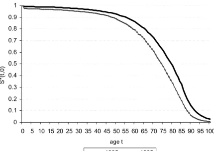
Figure 1: Survival Probabilities for the US Population (from age 0 tot), 1965 and 1995

0 0.1 0.2 0.3 0.4 0.5 0.6 0.7 0.8 0.9 1

0 5 10 15 20 25 30 35 40 45 50 55 60 65 70 75 80 85 90 95 100

age t

S

*(

t,0

)

1995 1965

The survival functions for 1965 and 1995 are calculated from age specific number of deaths and population, obtained from the World Health Organization Mortality Database. The database contains information broken down by 5 year age intervals, so we assume constant mortality rates within each interval. We calculate the 1965 numbers as averages for the period between 1960 and 1969, and the 1995 numbers as averages between 1990 and 1999. Figure 1 illustrates the shift in the (undiscounted) survival function for the US population between 1965 and 1995. This shift corresponds to a change in overall life expectancy at birth from 70 to 76 years. Note that the US experienced relatively modest gains in child mortality during this period, mainly because of the already extremely low starting point (mortality before 5 years went from 2.84 to 0.99 percent). Also, the age distribution of the American population in 1965, portrayed in Figure 2, had a relatively high share of old adults when compared to young adults. If anything, it seems that the particular example picked will tend to minimize the importance of the forces that we are trying to highlight.

Figure 2: Age Distribution of the US Population, 1965

0% 2% 4% 6% 8% 10% 12%

< 1 1-4 5-9 10-14 15-19 20-24 25-29 30-34 35-39 40-44 45-49 50-54 55-59 60-64 65-69 70-74 75-79 80-84 >84

age groups

of life literature. First, interest rates are assumed to be 3 percent per year, and this number is used to calculate the discounted survival functions (S(t, a)). As mentioned, the assumption of subjective rate of time preference equal to the interest rate implies constant consumption throughout life. This allows the consumption term in the willingness to pay expressions to be factored as ¡ε−1

c −1

¢

c

∞

R

i

Sθ(t, i)dt. Consumption is set to the 1965 value of total per capita

consumption (private plus government, in 1996 US$), obtained from the Federal Reserve Board Economic Database ($13,835). The value of εc can be estimated from compensating differentials for occupational mortality risks. Murphy and Topel (2001), using numbers from the literature on occupational risks, estimate εc to be 0.346.

For fertility (nT), the survival probability of children (pc), and the discounted survival prob-ability of adults up to the age when fertility is realized (S(τ, a)), we use the 1965 values of, respectively, the total fertility rate (2.9, ornT = 1.45), the survival probability between ages zero and 18 (0.96), and the discounted survival probability between ages 18 and 40 (0.50). We take

when they are 25 or 30, and take care of children in one way or another until they are roughly 50 or 55, the middle point would be around age 40.

The remaining parameters needed —b,e,φ, andα— are somewhat uncommon in applied work, so some exploratory calibration effort is required.

Estimates of b and e can be obtained from surveys of expenditures on children, such as the ones undertaken by the US Department of Agriculture (USDA). Lino (2001) presents the 1960 estimates of the USDA for the average costs of raising a child up to age 18, in 2000 US$. We use the CPI to deflate this value to 1996 US$. The USDA estimates imply that roughly 5 percent of the expenditures on children take place before age 2, while 95 percent take place between ages 2 and 18.13 _{We assume that costs up to age 2 are related to the costs of having a child (b),} and costs between ages 2 and 18 are related to costs of raising a surviving child (e). This yields

b = $6,956 and e = $126,812. Again, if anything, these estimates seem to underestimate the value ofbin comparison toe, and this will tend to minimize the importance of child mortality in welfare evaluations.

Finally, we need estimates ofα andφ. Identification of these parameters requires somewhat subtler information. It requires knowledge of how much individuals value their own utility vis-`

a-vis their children’s utility, and by how much this relative valuation changes as their number of children changes. We know of no direct study trying to estimate these relations. Therefore, to calibrate the values ofαandφ, we use the evidence presented by Cropper, Aydede, and Portney (1992) regarding the rate at which people implicitly discount future lives saved. They estimate the average discount rate applied to lives saved 25 years in the future to be 0.087, and the increase in this discount per additional child below 18 in the household to be 0.0145. We make the heroic assumption that these estimates correspond to, respectively,αS(τ, a)E(N_Tφ) andαS(τ, a)∂E(NTφ)

∂nT ,

evaluated at the average fertility level.14 _{These expressions define two non-linear equations inα} andφ, that can be numerically solved. For the case in question, we obtainα= 0.16 andφ= 0.24. There are various problems with this identification of α and φ. First, in the hypothetical exercise used in the interviews that entail Cropper, Aydede, and Portney’s (1992) estimates, there are no personal relations between the individuals being considered. Second, even in this context, it

13_{These shares are roughly constant across income levels and time. Also, the growth in expenditures on children} through time seem smaller than one might expect. In 1960, total expenditures per child up to age 18 were $133,768, while in 2000 this number was $150,899 (both in 1996 dollars).

14 _{Suppose that the value of a given reduction in mortality could be expressed as a function of the “number} of lives saved” (L). Consider a variable θ1 which reduces mortality today by some amount, and a variableθ2 which reduces mortality for future generations by another. An individual will be indifferent between the changes in mortality brought about byθ1andθ2if and only if _∂θ∂L₁ =αS(τ, a)E(NTφ)

∂L

∂θ2. This is the very loose sense

in which we assume thatαS(τ, a)E(NTφ) corresponds to the number estimated by Cropper, Aydede, and Portney

is not clear whether their estimates correspond exactly to the theoretical concepts that we would ideally want. Changes in survival probabilities cannot be summarized in terms of number of lives lost, with the same values for any individual at any given age. Additionally, the ideal exercise to estimate αandφ would consider permanent changes in mortality taking place at the present against permanent changes in mortality taking place at some future point, benefiting relatively more future generations. The survey used by the authors consider trade-offs regarding a one-shot reduction in the number of deaths in the present, against a one-shot reduction in the number of deaths in the future. Finally, Cropper, Aydede, and Portney (1992) themselves identify a series of signals indicating that their results probably overestimate the actual discount rate applied to future lives saved.15

Despite all these problems, we think of these numbers as an initial benchmark to can guide our discussion. We take Cropper, Aydede, and Portney’s (1992) 0.087 number to be a lower bound estimate of the intergenerational discount factor. In our view, and given all the caveats discussed in the last paragraph, the intergenerational discount applied between members of the same family is likely to be larger than this.

We calibrate the model using the parameters generated by this benchmark specification and then change the specification by varying the intergenerational discount rate. First, we consider the value suggested by Arrow (1995). Arrow suggests that the pure social discount rate across generation should be roughly 4%. Discounting this value from the perspective of an individual entering adulthood, we obtain αS(τ, a)E(N_Tφ) = 0.484, which is very close to one-fourth of the discount rate estimated in Cropper, Aydede, and Portney (1992) (thinking in terms of rates, we have √4

0.087 = 0.543). This yieldsφ= 0.04 andα= 0.95.

Following, we consider the intergenerational discount rate suggested by the evolutionary biol-ogy literature. According to this view, the altruism between two individuals can be genetically motivated only if it is given by the “coefficient of relationship” between them, or , in other words, by the pool of common genes that the two individuals share (see discussion in Bergstrom (1996)). This would give a pure intergenerational discount rate betweens parents and children equal to 50%, which, discounted from the perspective of an individual entering adulthood, yields αS(τ, a)E(N_Tφ) = 0.252. This in an intermediary case, close to one-half of the discount rate esti-mated by Cropper, Aydede, and Portney (1992) (again, in terms of rates, we have√0.087 = 0.293). This number generates φ= 0.08 andα= 0.49.

Introspection suggests that all three cases are rather conservative estimates. It is worth re-membering that αS(τ, a)E(N_Tφ) = 0.087 implies that parents values their own consumption more than 10 times more than the utility of each child. In any case, we do not think that this is the ideal way to calibrate the values ofαandφ. Instead, we consider our tentative approach an important first step in a direction that requires further research.

Table 1 presents the values of the main parameters and initial period variables used in the benchmark specification. Table 2 presents the marginal willingness to pay of an individual entering adulthood (age a) for the three sets of parameters, together with the values ofα andφ implied by the different parameterizations, and the increase in the calculated welfare gains due to the incorporation of fertility and altruism. Table 3 presents the total social value of the gains in survival rates for the same set of parameters, together with the increase in the calculated social gains due to the new dimensions considered.

Table 1: Values of Variables in Benchmark Parameterization Base Year: 1965

pc 0.96

S(τ, a) 0.50

c 13,835

nT 1.5

φ 0.24

α 0.16

b 6,956

e 126,812

εc 0.35

E(N_Tφ) 1.09

∂E(NTφ)

∂nT 0.181

µ 0.147

αS(τ, a)E(N_Tφ) 0.087 εn 0.25

the reductions in mortality that were observed between 1965 and 1995. This number is 20 percent higher than what would be obtained had fertility and altruism been ignored. As we increase the weight that parents give to their children, this difference increases exponentially. If we assume that S(τ, a)E(N_Tφ) = 0.252, the willingness to pay of an 18 year old individual in 1965 becomes US$38,470, or 71 percent higher than in the traditional setup. In the last case, when we use the discount rate suggested by Arrow (1995), the calculated willingness to pay of a young adult is US$66,773, or 197 percent higher than what would be obtained in the traditional setup.

Table 2: Value of Mortality Reductions in the US between 1965 and 1995 for an 18 Year Old Individual, Different Sets of Parameters

parameterization αS(τ, a)E(N_Tφ) φ α M W Pa Increase from (1996 $) Traditional

Cropper et al. (1992) 0.087 0.24 0.16 27,035 20%

Evolutionary Biology 0.252 0.08 0.49 38,470 71%

Arrow (1995) 0.484 0.04 0.95 66,773 197%

When we move to the analysis of the social value of mortality reductions, these numbers decline. This is because a large fraction of the population is composed by old adults, who already surpassed the assumed child rearing age (τ = 40).16 _{Table 3 shows that, in this case, the most} conservative set of estimates (αS(τ, a)E(N_Tφ) = 0.087) implies that the social value obtained using our methodology is 6 percent higher than what would be obtained otherwise. But, again, this number increases exponentially with increases in the weight given to children by their parents. With the intermediate set of estimates (S(τ, a)E(N_Tφ) = 0.252), the calculated social value of the reductions in mortality is 22 percent higher than what it would be in the traditional approach. With parents discounting children at the rate suggested by Arrow (1995) (αS(τ, a)E(N_Tφ) = 0.484), the calculated social value becomes 65 percent higher than what would be obtained ignoring fertility and altruism.

Table 3: Social Value of Mortality Reduction in the US between 1965 and 1995, Different Sets of Parameters

parameterization αS(τ, a)E(N_Tφ) φ α Social M W P Increase from (Bill., 1996 $) Traditional

Cropper et al. (1992) 0.087 0.24 0.16 4,920 6%

Evolutionary Biology 0.252 0.08 0.49 5,659 22%

Arrow (1995) 0.484 0.04 0.95 7,620 65%

In terms of values, the intermediate set of estimates (S(τ, a)E(N_Tφ) = 0.252) implies that the gains in life expectancy experienced in this thirty-year period had a social value of 5.66 trillion dollars (in 1996 US$). This value corresponds to almost 2 times the value of the US GDP in 1965. And 1 trillion dollars come directly from the effects of fertility and altruism in the valuation of changes in mortality.

Though the results are quantitatively significative, and indicate the relevance of fertility and altruism in value of life-type calculations, we must repeat that several dimensions of our empirical implementation tend to underestimate the factors that we are trying to highlight. Indeed, we see the evidence as an extremely strong case in favor of the incorporation of fertility and altruism into the analysis. In our subjective evaluation, a more precise estimation of the parametersb, e,α,

andφ, and the application of the methodology to countries or periods with larger changes in child mortality, would both tend to increase the relative importance of fertility and altruism.

5

Final Comments

To illustrate the empirical relevance of fertility and altruism in the value of life problem, we used our methodology to value the reductions in mortality rates experienced by the US between 1965 and 1995. Our results show that altruism and fertility can easily double the value of mortality reductions for a young adult, when compared to results obtained using the traditional value of life methodology.

Yet, some additional effort on the estimation of “new” parameters is necessary, in order to generate a more precise estimate of the relative importance of fertility and altruism in the problem. These parameters are related to the costs of having and raising children, and to the way in which parents discount their children’s utility when compared to their own. We believe that these issues deserve further attention, and may be important areas for future empirical research.

References

[1] Arrow, Keneth J. (1995). “Intergenerational Equity and the Rate of Discount in Long-term Social Investment.” IEA World Congress, December 1995, 23p.

[2] Arthur, W. Brian. (1981). The Economics of Risks of Life.American Economic Review, Vol. 71, 54-64.

[3] Becker, Gary and Robert Barro (1988) A Reformulation of the Economic Theory of Fertility. Quarterly Journal of Economics, Vol. 103, 1-25.

[4] Becker, Gary and Kevin. Murphy (1988). The Family and the State. Journal of Law and Economics, Vol. 31, 1-18.

[5] Becker, Gary, Tomas Philipson, and Rodrigo R. Soares (2003). “Quantity and Quality of Life and the Evolution of World Inequality.” Unpublished manuscript, University of Chicago. [6] Bergstrom, Theodore C. (1996). Economics in a Family Way.Journal of Economic Literature,

Vol. 34, No. 4. (Dec., 1996), pp.1903-1934.

[7] Cropper, Maureen L., Sema K. Aydede, and Paul R. Portney (1992). Rates of Time Prefer-ence for Saving Lives.American Economic Review Papers and Proceedings, Vol. 82, 469-472. [8] Cropper, Maureen L. and Frances G. Sussman (1988). Families and the Economics of Risks

to Life.American Economic Review, Vol. 78, 255-260.

[9] Garrett, Allison M. (2001). “Health Improvements and the National Income and Product Accounts: 1880 to 1940.” Unpublished manuscript, University of Chicago.

[10] Kalemli-Ozcan, Sebnem (2002). Does Mortality Decline Promote Economic Growth? Jour-nal of Economic Growth, Vol. 7, 411-439.

[11] Lino, Mark (2001). USDA’s Expenditure on Children by Families Project: Uses and Changes Over Time.Family Economics and Nutrition Review, Vol.13, No.1, 81-86.

[13] Murphy, Kevin M. and Robert Topel (2001). “The Economic Value of Medical Research.” Unpublished manuscript, University of Chicago.

[14] Nordhaus, William D. (1999). “The Health of Nations: The Contribution of Improved Health to Living Standards.” Unpublished manuscript, Yale University.

[15] Rosen, Sherwin (1988). The Value of Changes in Life Expectancy. Journal of Risk and Uncertainty, Vol. 1, 285-304.

[16] Rosen, Sherwin (1994). The Quantity and Quality of Life: A Conceptual Framework. In: George Tolley, Donald Kendel, and Robert Fabian (eds.).Valuating Health for Policy: An Economic Approach. Chicago, University of Chicago Press, 221-248.

[17] Sah, Raaj (1991). The Effects of Child Mortality Changes on Fertility Choice and Parental Welfare.Journal of Political Economy, Vol. 99, 582-606.

[18] Schelling, Thomas C. (1968). The Life You Save May Be Your Own. In: Samuel B. Chase, Jr (editor).Problems in Public Expenditure Analysis. Brookings Institution, Washington D.C., 1968, p.127-61.