❊♥s❛✐♦s ❊❝♦♥ô♠✐❝♦s
❊s❝♦❧❛ ❞❡
Pós✲●r❛❞✉❛çã♦
❡♠ ❊❝♦♥♦♠✐❛
❞❛ ❋✉♥❞❛çã♦
●❡t✉❧✐♦ ❱❛r❣❛s
◆◦ ✹✹✼ ■❙❙◆ ✵✶✵✹✲✽✾✶✵
❱✐♥t❛❣❡ ❈❛♣✐t❛❧✱ ❉✐st♦rt✐♦♥s ❛♥❞ ❉❡✈❡❧♦♣✲
♠❡♥t
❙❛♠✉❡❧ ❞❡ ❆❜r❡✉ P❡ss♦❛✱ ❘❛❢❛❡❧ ❘♦❜
❖s ❛rt✐❣♦s ♣✉❜❧✐❝❛❞♦s sã♦ ❞❡ ✐♥t❡✐r❛ r❡s♣♦♥s❛❜✐❧✐❞❛❞❡ ❞❡ s❡✉s ❛✉t♦r❡s✳ ❆s
♦♣✐♥✐õ❡s ♥❡❧❡s ❡♠✐t✐❞❛s ♥ã♦ ❡①♣r✐♠❡♠✱ ♥❡❝❡ss❛r✐❛♠❡♥t❡✱ ♦ ♣♦♥t♦ ❞❡ ✈✐st❛ ❞❛
❋✉♥❞❛çã♦ ●❡t✉❧✐♦ ❱❛r❣❛s✳
❊❙❈❖▲❆ ❉❊ PÓ❙✲●❘❆❉❯❆➬➹❖ ❊▼ ❊❈❖◆❖▼■❆ ❉✐r❡t♦r ●❡r❛❧✿ ❘❡♥❛t♦ ❋r❛❣❡❧❧✐ ❈❛r❞♦s♦
❉✐r❡t♦r ❞❡ ❊♥s✐♥♦✿ ▲✉✐s ❍❡♥r✐q✉❡ ❇❡rt♦❧✐♥♦ ❇r❛✐❞♦ ❉✐r❡t♦r ❞❡ P❡sq✉✐s❛✿ ❏♦ã♦ ❱✐❝t♦r ■ss❧❡r
❉✐r❡t♦r ❞❡ P✉❜❧✐❝❛çõ❡s ❈✐❡♥tí✜❝❛s✿ ❘✐❝❛r❞♦ ❞❡ ❖❧✐✈❡✐r❛ ❈❛✈❛❧❝❛♥t✐
❞❡ ❆❜r❡✉ P❡ss♦❛✱ ❙❛♠✉❡❧
❱✐♥t❛❣❡ ❈❛♣✐t❛❧✱ ❉✐st♦rt✐♦♥s ❛♥❞ ❉❡✈❡❧♦♣♠❡♥t✴
❙❛♠✉❡❧ ❞❡ ❆❜r❡✉ P❡ss♦❛✱ ❘❛❢❛❡❧ ❘♦❜ ✕ ❘✐♦ ❞❡ ❏❛♥❡✐r♦ ✿ ❋●❱✱❊P●❊✱ ✷✵✶✵
✭❊♥s❛✐♦s ❊❝♦♥ô♠✐❝♦s❀ ✹✹✼✮
■♥❝❧✉✐ ❜✐❜❧✐♦❣r❛❢✐❛✳
Vintage Capital, Distortions and Development
Samuel de Abreu Pessoa
∗Rafael Rob
†May 21, 2002
A bst r act
This paper asks to what extent distortions to the adoption of new technology cause income inequality across nations. We work in the framework of embodied technological progress with an individual, C.E.S. production function. We estimate the parameters of this production function from international data and calibrate the model, using U.S. National Income statistics. Our analysis suggests that distortions account for a bigger portion of income inequality than hitherto has been assessed.
JEL Classification numbers: D24, D33, E25, O11, O47, O49
K ey words: Vintage Capital, Embodied Technological Progress, Putty-Clay, Total Fac-tor Productivity, Elasticity of Substitution.
1
I nt r oduct ion
In this paper we assess to what extent distortions to the purchase of capital-goods account for the huge per-capita income differences among countries of the world. We approach this question by considering a world in which there is exogenous technological progress and where the decision to adopt new technology depends on the price of capital that embodies this technology. We construct a model of this adoption decision and use it to determine
∗
Graduate School of Economics (EPGE), Fundação Getulio Vargas, Praia de Botafogo 190, 1125, Rio de Janeiro, RJ, 22253-900, Brazil. Fax number: (+) 55-21-2553-8821. Email address: [email protected].
whether the observed variation in the price of adopting technology accounts for the observed variation in per-capita incomes.
In analyzing this question, we hypothesize that technological progress is embodied, rather than disembodied. In other words, we hypothesize that technological progress is effective only if new capital-goods that embody the new technology are installed. In such a world, the effect of distortions is strong for the simple reason that when no new capital-goods are installed (due to distortions), there is no growth in income. By contrast, if technological progress were disembodied, it would apply to old capital-goods and, hence, would raise incomes even without the installation of new capital-goods. Our main objective is to quantify this reasoning; i.e., contrast the quantitative effects of distortions in a disembodied versus an embodied model.
This approach wasÞrst suggested in a paper by Jovanovic and Rob (1997) and continued in papers by Parante (2000) and Mateus-Planas (2001). Compared with those papers, we offer the following improvements. First, instead of picking a production function in advance (for example, the Leontieff production function), we estimate a production function from empirical data. More speciÞcally, we consider the C.E.S. family of production functions, and pin down one member of this family based on international data on investments and prices. This makes the model more amenable to empirical and quantitative exercises for two reasons. First, because the production function is derived from data, the results pertaining to it are more empirically relevant. Second, because the production function we use allows
Þrms to choose the quantity of capital on top of the timing of adoption, the model mimics more accurately the way Þrms adjust their capital in the real world.
A second improvement compared to previous models with embodied technological progress is that our theory cranks out a price-proÞle for capital of different vintages. This price-proÞle is then used to evaluate the inventory of capital goods in the economy, which is the com-mon practice in National Income statistics. As a result of this procedure, we make a clear and operational distinction between three types of depreciation: physical, technological (or obsolescence) and economic (or scrapping). By contrast, previous models construct an ad-hoc measure of the value of the inventory of capital goods and, as a result, lump together different types of depreciation.
vary across countries, holding other parameters constant) can easily account for the observed income inequality when distortions are allowed to vary over a reasonable range. This is to be contrasted with the aforementioned models of embodied technological progress where that is not the case. It is also to be contrasted with models of disembodied technological progress, which require an unrealistic capital share of income, namely 2/3, instead of the “traditional” 1/3 in order to have the same explanatory power (see Chari et al. (1997)). Related to this, a version of our model is able to account for growth miracles based purely on factor accumulation, as documented by Young (1995). A second indicator of the success of our theory is that, even if we accommodate other, non-economic factors, distortions remain an important explanatory variable. This can be contrasted with Hall and Jones (1999) who argue that these factors play an overwhelming role by comparison with economic factors. The reason we are able to improve upon the Hall and Jones (1999) exercise is that our embodied model generates an endogenous Total Factor Productivity (TFP) term, which accounts for some of the variation in income. By contrast, when technological progress is disembodied, there is no such thing as endogenous TFP and, thus, the entire unexplained variation in incomes is absorbed into the exogenously speciÞed TFP term.
We proceed as follows. In the following subsection we describe verbally the mechanics of our model. In Section 2 we formalize the model. In section 3 we solve the Þrm’s maxi-mization program. In section 4 we solve for general equilibrium. In section 5 we aggregate various variables and derive various National Income statistics. In Section 6 we calibrate the model. In Section 7 we estimate the individual production function. In section 8 we simulate the model, showing what per-capita incomes it predicts as distortions vary from country to country. In Section 9 we report various other predictions of our model, including the capital-output ratio and the price-earning ratio. In Section 10 we perform a development decomposition exercise, showing how much inequality is explained by distortions when we take a more comprehensive view of the sources of inequality. Section 11 concludes.
1.1
Ver bal descr ipt ion of t he M odel and it s M echanics
the timing of adoption and, at each date of adoption, it chooses how much capital to install. The economy is populated by a continuum of Þrms, which upgrade their technology in sequence. As a result of these sequential upgradings, we have, at any moment in time, a window of capital goods in the economy. The width of this window corresponds to the waiting period between upgrades and the height of the window corresponds to how much capital is being installed by each Þrm. In addition, at any moment in time, we have a (general equilibrium) price-proÞle of capital-goods; i.e., a function relating the vintage of a capital-good to its price. The essence of the model is to determine how the window and prices of capital-goods are affected by distortions and other parameters. Once we determine these effects, we proceed to determine the effect of distortions on various National Income statistics. In particular, we determine the effect of distortions on the holding period of capital-goods, the per-capita income, the investment-capital ratio, the investment-output ratio, wage-rates, and the price-earning ratio. These effects can then be contrasted both with micro and macro-data.
2
T he M odel
We consider an inÞnite horizon, continuous-time economy.
A gent s and G oods. The economy is populated by a continuum of identical, inÞ nitely-lived individuals of measure 1. Each individual consumes output, and supplies inelasticly one unit of labor. The productivity of individuals’ labor is determined by their educational level.
In addition to individuals, there is a continuum of inÞnitely-livedÞrms. Each Þrm sells output, hires individuals, and buys capital. Firms are owned by individuals, as speciÞed below. Individuals andÞrms take prices as given. Since production in eachÞrm is according to a constant returns to scale technology, the measure (and size) of Þrms is indeterminate. For convenience, we normalize this measure to be 1.
There is one output in the economy, which is used both for consumption and capital accumulation. When a Þrm buys capital, output is withdrawn from consumption on a one-to-one basis.
the meaning of “quality” is speciÞed immediately below. We assume:
A(s) =A0egs,
where g is the rate of technological progress.
Firms periodically upgrade their technology by buying new capital. Capital installed at date s reßects the date-s frontier technology and is said to be vintage-s capital. AÞrm that last upgraded its technology at date s is said to be a vintage-s Þrm.1
A single fi r m at a gi ven point in t im e. AÞrm is characterized, at a given point in timet, by its technologys(s ≤t), and its capital-worker input-combination, denoted(K, L), whereK is the capital-workerratioandLis the number of workers. Assume all workers have the same educational levelh, and assumehis constant through time. Then, an(s, K, L)-Þrm is using LA(s)eφ(h) efficiency units of labor. h is measured by years of schooling andeφ(h) is
a Mincerian function which translates years of schooling into labor productivity. According to this speciÞcation, a newer-vintage technology is of higher quality in that it translates the time of a worker into more efficiency units of labor. A higher educational level has the same effect.
P r oduct ion in a single fi r m. AÞrm produces output according to a C.E.S. production function. Namely, the date-t per-worker ßow of output of an (s, K, L)-Þrm is:
Y(s, t) =e−δ(t−s)Bh(1−α)(A(s)eφ(h))σ−1
σ +αK
σ−1
σ
i σ
σ−1
, (1)
whereσ is the elasticity of substitution andαis the distribution parameter. B is total factor productivity (TFP), i.e., it measures the efficiency with which a Þrm converts inputs into output, and δ is the physical depreciation factor.2 The values of these parameters are the
same for all Þrms within one country, and remain constant through time.3 On the other
hand, as we go across countries (which we do later) the values of parameters change. Hence differences across countries are captured by differences in parameter values.
To make the language less cumbersome we refer sometimes to capital per-worker simply
1To be precise one should distinguish between aÞrm and a plant. AÞrm is an inÞnitely-lived entity that
upgrades its plant every once in a while. A plant consists of a certain vintage capital and ceases to exist once this capital is upgraded. For simplicity we suppress this distinction.
as “capital” and to output per-worker as “output.”
U pgr ading. Consider a point in time, says, at which aÞrm upgrades its technology. At that point the Þrm also chooses how much capital of that vintage to install and how many workers to employ. Once the Þrm makes that determination it is committed to the
vintage-s technology and to the (K, L) input-combination - until its next technological upgrade. Therefore, aÞrm has fullßexibility ex-ante, and full rigidity ex-post.4 Between upgrades the
Þrm makes no economic decisions; it merely collects the output ßow speciÞed by (1), and pays wages.
The cost of upgrading to a new technology is p units of output per-unit capital of the new vintage. Thus, if a Þrm upgrades at dates and installsK units of capital per-worker, it pays pKL. pKL is paid up-front (ats), and pis independent of s.
When a Þrm upgrades to a new technology it dumps the capital of its old technology; there is no such thing as a second-hand market in capital-goods,5 and there is no such thing
as combining capital of different vintages. Also, although capital is “made of” output and output is the same through time, there is no way of converting capital-goods of an old vintage into a newer vintage. There is also no way of converting capital-goods back into output that can be consumed. The decision to create capital goods is irrevocable.
T he Fir m ’ s M axim izat ion Pr oblem. The objective of a Þrm is to maximize the discounted value of revenues net of wages and capital upgrading costs. Discounting is with respect to the constant, instantaneous interest rate r, which the Þrm takes as given.
The economic decision facing aÞrm is as follows. At a given point in time, say t, theÞrm operates with a certain combination (s, K, L). Then it has to decide on its next upgrade date say s+T, where T is labelled the “waiting period” (and 1
T is labelled the “frequency of upgrades.”) The Þrm has also to decide on how much capital to install and how many workers to employ at s+T.
The trade-off governing these decisions is as follows. The capital stock the Þrm has on its hands is already paid for so it “comes for free.” On the other hand, as time goes on the technological frontier keeps moving out so this capital becomes more and more obsolete. On top of that, the Þrm had pre-committed itself to employ a certain number of workers whose equilibrium wage keeps increasing (see below).6 Therefore, a point comes where it no longer
4Known in the 1960s literature as the “putty-clay” formulation. 5We introduce this market later.
Nonethe-pays to keep the old technology, i.e., it Nonethe-pays to upgrade. We determine below the optimal upgrade date, or, equivalently, the optimal waiting period, T.
Considering output used for consumption as the numeraire, the dynamic programming formulation of the Þrm’s problem is as follows:
V(s, K, t) = max T,K0
½Z T+s
t
e−r(τ−t)[Y(s,τ)−w(τ)]dτ
+e−r(T+s−t)[V(T +s, K0, T +s)−pK0]ª, (2)
where w(τ) is the wage rate at date τ. V is the per-worker value function. The Þrm takes
p, r, and w(·) as given.
D ist or t i ons. As stated earlier there is, at aÞxed point in time, a one-to-one (social) rate of transformation between consumption and investment. Nonetheless, aÞrm (privately) pays
p for capital, rather than paying 1. The reason is that there are distortions (or subsidies) to the adoption of technology, which equal p−1. At the level of the theory, distortions are broadly interpreted; distortions could be taxes or tariffs on the acquisition of machines, bureaucratic hurdles on the construction of new structures, regulatory delays in implementing new discoveries, corruption, etc. When we (later) quantify the theory, distortions are more narrowly interpreted as taxes and tariffs. At that point we also verify that this narrow interpretation does not constrain the empirical usefulness of our quantitative exercises.
Several comments on our modeling choices are in order.7
1. Production in our model is according to the C.E.S. production function, which is in contrast with the “usual” production function in the growth and development litera-ture, namely Cobb-Douglas. Our idea is to allow a parametric family of production functions and, then, pin down a member of this family, based on empirical data; in particular, we are not ruling out the Cobb-Douglas case, which is a special case of a C.E.S. production function when σ = 1.8 As we show below a wealth of empirical
less, upgrading still occurs as long asσ<1(even if laborisdivisible and perfectly mobile). Thus, our results do not necessarily hinge on the ex-post rigidity of labor demand.
7Our model is closely related to a class of models poularized in the 1960, in particular, Phelps (1963),
Solowet all (1966), Bliss (1968) and Bardhan (1969). Our working paper explains in what ways we extend that class of models.
8We are also not ruling out the Leontief case, which is a special case of a C.E.S. production function when
implications hinges on the production function at hand. Thus, we are able to assess the plausibility of the production function we pin down by comparing the implications it yields to those yielded by the Cobb-Douglas (or some other) production function.
2. Technological progress in our model is embodied in capital, but has an effect on la-bor. Intuitively, what the new-vintage capital does is to enable workers to use better equipment, thereby raising their productivity. This is known in the literature as “labor-augmenting” (or “labor-saving”) technological progress. Two major reasons for consid-ering the labor-augmenting, as opposed to the capital-augmenting, case are: (i) Since we focus on a balanced growth-path (see below), since such path does not exist when technological progress is capital-augmenting (unless the production function is Cobb-Douglas), and since it does exist when technological progress is labor-augmenting, the choice of which technological progress to consider is pinned down by what we focus on. (ii) If technological progress were capital-augmenting and labor were mobile between vintages the model would be simpler in that there would be an aggregate quantity of capital and an aggregate production function. See Fisher (1965) for a general result, and Greenwoodet al. (1997) who use such model to study growth features of the U.S. economy. The advantage of using our more complex model is that it parallels the treat-ment of capital goods in U.S. National Accounting, NIPA (whereas the simpler model does not). In particular, NIPA reaches an aggregate value of capital by distinguishing between capital goods of different vintages, pricing them differentially and adding up their values, which is exactly what we do here.9
3. As time progresses a Þrm is able to produce less and less (unless it upgrades) due to what we call “physical depreciation.” More conventionally, physical depreciation affects the capital stock, not the output that results from it.10 The primary reason
for our speciÞcation is analytical convenience. As we shall see, we are able to solve
9Another obvious advantage is that the model with mobile labor has been extensively studied, whereas
the model with immobile labor has not.
10A plausible story to tell about our way of treating depreciation (and, at the same time, about the
the model analytically under this assumption, whereas under the more conventional assumption it can only be solved numerically. As it turns out, it makes little difference whether output or capital depreciates. We have solved (numerically) the model under the alternative assumption that capital depreciates, and found the quantitative results to be very close; we explain the reason for this later.
To complete the model’s description one needs to specify the economy’s initial conditions, and individuals’ maximization problems (in their capacity as consumers). We do that after we state the solution to the Þrm’s problem.
3
Solut ion t o t he Fir m’s M aximizat ion Pr oblem
We seek a balanced growth-path, along which all real variables grow (exponentially) at the constant rate,g. With this goal in mind, we consider, from this point onwards, only constant-growth wage paths, w(τ) = w0egτ, wherew0 is endogenous and yet to be determined.
deals with these issues and characterizes the solution across different parameter values. The following Proposition states the net result for a range of parameter values which includes the empirically relevant case. In stating the Proposition we use the following notation:
f(x)≡
h
1−α+αxσ−σ1
i σ
σ−1
,
where f(x)≡ AY(0)
0Beφ(h) andx≡
K A0eφ(h).
For simplicity we set, from this point onwards,A0= 1.
P r op osit ion 1 Assume 0 ≤ σ < 2 and w(s) = f(k)e−(g+δ)Teφ(h)+gs, where k and T are
specified immediately below. (i) Assume also that p ≤ p ≡ rB+δασ−σ1 for 0 ≤ σ <1, or that
p ≥ p for 1 < σ < 2. Then there exist unique optimal waiting periods between upgrades, which are constant, strictly positive and finite. The optimal waiting periodT is the solution to the following equation:
0 = e−δT
B ·
p
αBD(r+δ, T)
¸σ
−egT 1
D(r−g, T)
·
D(r+δ, T)
µ
p
αBD(r+δ, T)
¶σ
B−p ¸
, (3)
whereD(x, T)≡ 1−e−xT x .
(ii) Consider a dates at which thefirm upgrades. T hen the optimal capital-worker ratio is:
K(s) =keφ(h)+gs, (4)
where k ≡
h
Zσ−1−α 1−α
i σ
1−σ
and Z ≡ αBDp
(r+δ,T). The optimal labor demand is indeterminate, L(s)∈[0,∞).
T he maximized output at s is:
Y(s, s) = Bf(k)eφ(h)+gs. (5)
(iii) I f the hypotheses underlying (i) are not satisfied, thefirm never upgrades its capital or demands an infinite quantity of capital.11
11We are not discussing these possibilities in greater detail because we are interested in a balanced-growth
As the Proposition states, the scale of production is indeterminate whenever w(s) =
f(k)e−(g+δ)Teφ(h)+gs. This is a standard feature of models with price-takingÞrms and with constant returns to scale. If the average cost in such model is equal to the product price -and w(s) = f(k)e−(g+δ)Teφ(h)+gs is the analogue of this condition in our model - the Þrm is indifferent between all scales of production.12 Another standard feature is that although the
scale of production is not determinate the capital-worker ratio K(s) is.
Other features of the solution are as follows: (i) The Þrm’s optimum choices are de-termined sequentially. We Þrst solve for the optimal waiting period T using equation (3). Then, we plug this T into (4) and solve for the optimal quantity of capital. Therefore, T is scale-independent so it becomes an “intensive” variable, like K. (ii) The optimal quantity of capital K(s) grows at the constant rate g; theÞrm is on a balanced growth-path. (iii) The optimal choice of T andK depend only on the ratio Bp, not on each one separately. (iv) h
affects the choice ofK, but not the choice of T.13
Regarding the comparative statics of the optimum, and maintaining the assumptions underlying Proposition 1, we have the following result:
P r op osit ion 2 (i) K(s) is decreasing in p. (ii) I f σ <1, T increases in p and if σ >1, T decreases in p. If σ = 1, T is independent of p.
The speciÞc mechanism via whichpaffectsT relates to capital and labor being substitutes or complements. In particular, when σ >1 labor and capital are substitutes. Hence, when
p goes up the Þrm uses less capital, and, because capital and labor are substitutes, it uses more labor. In turn, one way of using more labor is to upgrade more frequently (because then the “effective” quantity of labor increases).
Proposition 2(ii) suggests aÞrst glimpse at why the Cobb-Douglas case or, more generally, σ ≥ 1 might not be the most realistic production function in our context. Indeed it would
12If w(s) > f(k)e−(g+δ)Teφ(h) +gs, the Þrm produces zero. If w(s) < f(k)e−(g+δ)Teφ(h) +gs, the Þrm
produces inÞnite quantity.
13The reason for this is thateφ(h) multipliesL, rather than K or the outputY. This provides a testable
implication of the way we incorporatehinto our production function, the implication being that as one goes across countries with different educational levels one should observe no variation - on account ofhalone - in the frequency of technological upgrades. This implication can be used to contrast our way of incorporating hinto the production function with alternative ways.
seem that aspgoes up theÞrm would want to spread the higher cost of buying capital over a longer holding period. However, as Proposition 2 states, that holds true only if σ<1. Later in the paper we provide empirical evidence (and further theoretical arguments) corroborating this intuition, i.e., supporting σ<1.
4
G ener al Equilibr ium
We consider now the whole economy and determine equilibrium prices and the mechanics of consumption and investment over time and across Þrms.
4.1
T he household sect or
We start with the problem facing a typical individual in her capacity as a consumer. We assume such individual has a C.E.S. ßow utility function, u(c) = c1−γ
1−γ, and a constant rate
of time-preference parameter, ρ. The life-time utility of such consumer from a consumption stream, c(·), is:
∞
Z
0
e−ρtc(t)1
−γ
1−γ dt.
The consumer has some initial wealth, call it ω, which comes from owning equities, as we specify in the next two subsections. On top of that wealth, the individual receives a stream of wages w(·). The consumer chooses a consumption stream that maximizes her life-time utility subject to the life-time budget constraint:
0 =
∞
Z
0 e−rt
[c(t)−w(t)]dt−ω. (6)
As is well-known, the solution to the household’s problem is:
c(t) =c0e
r−ρ
γ t, (7)
4.2
P r icing of Capit al G oods
When a Þrm upgrades its capital it Þnances this activity by going to the bond market and borrowing at the constant interest rate r. Equivalently, a Þrm can go to the equity market and issue shares. Let the unit of measurement be such that one share is backed by one unit of capital. Then a share yields a stream of dividends which equals the marginal productivity of this capital. Denote the date-τ marginal productivity of vintage-s capital by R(s,τ). Then, considering a share of a vintage-s Þrm, its price must be the discounted value of the dividends it yields:14
p= s+T
Z
s
R(s,τ)e−r(τ−s)dτ.
By the same token, if we consider a later date, say t, wheres < t < s+T, the date-tprice of a share issued at date-s,p(s, t), is the discounted value of the remaining dividends it yields:
p(s, t) = s+T
Z
t
R(s,τ)e−r(τ−t)dτ. (8)
We interpretp(s, t)either as the share price of a vintage-sÞrm, or, equivalently, as the price of the capital backing this share. In the second interpretation we consider p(s,·), for aÞxed
s, as tracking the price of vintage-s capital over its life-time.15 We consider p(·, t), for a
Þxed t, as a “price-proÞle” of capital of different vintages at date t. A familiar example of such price proÞle is the blue book, which lists the prices of cars of different “models,” i.e., it shows how the price of a car relates to its vintage (or, equivalently, its age).
4.3
I nit ial Condit ions
To focus on a balanced growth-path we assume that Þrms are initially staggered across vintages, so their upgrading decisions come in sequence. SpeciÞcally, we assume that at
t = 0 Þrms are uniformly distributed across vintages [−T,0) with a constant density = 1
T.
14The price of a share is understood as its shadowprice since in our economy we don’t need a separate
equity market to decentralize feasible allocations.
15Fixing s,p(s,·) is the function p(s, t) ast varies over[s, s+ T]. Fort > T + s, p(s, t) = 0. Analogous
The amount of capital per worker of a vintage-s Þrm, for−T ≤ s <0, is the K(s)speciÞed in equation (4). This pins down the economy’s initial conditions.
SinceÞrms upgrade in sequence, a density 1
T ofÞrms upgrades and a density
1
T of workers gets re-assigned to new vintage capital - at each point in time. Thus, a uniform distribution over vintages (or, equivalently, over capital of different ages) is preserved for the indeÞnite future.
4.4
Equilibr ium P r ices
WeÞnd now equilibrium wage rates, interest rates and shadow prices of capital and dividends. L abor M ar ket. At each instant, say s, a density 1
T of workers seek new employment as their employment with Þrms that dump their old capital is terminated. These workers give rise to a perfectly inelastic supply curve of workers, with a quantity intercept of 1
T. The equilibrium wage rate at s must be such that the set ofÞrms that are upgrading their technology (the same Þrms that used to employ these workers), demands this quantity of labor. Under the labor demand we derived in Section 3 this happens if and only if:
w(s) =f(k)e−(g+δ)Teφ(h)+gs. (9)
A noteworthy property of (9) is that the equilibrium wage rate at date s equals the per-worker output of an s−T-vintage Þrm. Thus, such Þrm dumps its capital at s even if it does not have the option to upgrade.
B ond M ar ket. Since output net of investment grows at the rateg, and since consump-tion grows at the rate r−ρ
γ , see equation (7), market clearing dictates we haveg =
r−ρ
γ . Thus,
r =γg+ρ.
D ivi dends. The dividend corresponding to vintage-s capital at time t is the marginal product of that capital. Given constant returns to scale, the total dividend distributed by a vintage-s Þrm is the output net of wages:
R(s, t)K(s) = e−δ(t−s)Bh(1−α)(eφ(h)A(s))σ−1
σ +αK(s)
σ−1
σ
i σ
σ−1
−w(t)
= e−δ(t−s)Bf(k)[1−e−(g+δ)(s−(t−T))]K(s), (10)
P r ice P r ofi le. Substituting (10) into (8) we get:
p(s, t) = pe−δ(t−s)D(r+δ, T −(t−s)) D(r+δ, T)
1−H(T −(t−s))
1−H(T) , (11) where:
H(T)≡ D(r−g, T)
D(r+δ, T)e
−(g+δ)T. (12)
Consider a point in time t and a vintage s, t−T < s < t. Then (10) and (11) show that dividends and capital prices are independent oft. Rather, they depend on the ageof capital only, t−s. Consequently, from this point onwards we write p(t−s), instead of p(s, t) and
R(t−s), instead ofR(s, t). At times it will be convenient to work with the variablea, which denotes the age of capital, e.g., p(a).
Figure 1 below shows two p(a) curves, one for a high-p country (p = 3), the other for a low-p country (p = 1). The parameter values underlying these curve are those we report in Sections 6 and 7.
0 20 40 60 80
Age
0.5 1 1.5 2 2.5 3
p
H
a
L
p=1
p=3
Figure 1:Price ProÞles. Parameters values are as calibrated for the U.S.
Both curves decrease, intersect the vertical axis atp, and intersect the horizontal axis at
a =T, i.e., at the age at which capital is retired.16 Note that the high-pcurve lies everywhere
16One can show that:
lim
T→∞p(a) = e −(g+δ)T
above and declines at a slower rate than the low-pcurve. Moreover, the high-pcurve declines at a slower rate even if we control for the higher price-intercept by dividing by p (in which case the two curves start at the same point on the vertical axis).
By contrast, if we consider σ > 1 we get counter-factual shapes of price-proÞles. A high-pprice-proÞle starts (obviously) higher than a low-p price-proÞle. However, the high-p
price-proÞle declines faster and, as a result, intersects the low-pprice-proÞle. Furthermore, it intersects the horizontal axis at a lower a, which is due to the fact that the life-time of capital is shorter the higher p is; see Proposition 2. This contrast between the shapes of price proÞles, depending onσ being below or above 1, provides further evidence in favor of σ <1.
Given equity prices, as given by (11), ω is determined as the value of initial equity holdings:
ω=
0
Z
−T
p(s,0)K(s)ds.
In turn, c0 is determined so that the consumer exhausts her budget.
5
A ggr egat ion
Given the above equilibrium, we construct now the theoretical counterparts of various National-Income Statistics.
Per -capit a out put . AttÞrms in the economy operate with vintage-stechnology, where
s ∈ [t−T, t]. A vintage-s Þrm employs T1 workers and produces a ßow of output Y(s, t). Thus, using (5), the aggregate per-capita output ßow att is:
y(t) = 1
T
Z t
t−T
Y(s, t)ds
= 1
T
Z t
t−T
e−δ(t−s)Bf(k)eφ(h)+gs ds
= yeφ(h)+gt, (13)
where:
y≡Bf(k)D(g+δ, T).
I nvest m ent . Att a density T1 of Þrms upgrades its capital, and each suchÞrm installs the quantity K(t) of new capital. Using (4), this implies that the per-capita investment at
t is:
i(t) = k
Te
φ(h)+gt
. (14)
I nvest m ent -Out put r at io. Using (13) and (14) it follows that the investment-output ratio is:
i ≡ i(t)
y(t) =
k T B
Tf(k)D(g+δ, T)
= 1
Bψ(k)D(g+δ, T), (15)
where
ψ(x)≡ f(x)
x = [(1−α)x
−σ−1
σ +α]
σ
σ−1.
Fact or -Shar es of I ncom e. Capital-income is the sum of dividends on capital employed by all Þrms. Since there is a density 1
T of vintage-s Þrms at time t, where s ∈ [t−T, t], capital-income at t is:
1
T
Z t
t−T
R(t−s)K(s)ds.
After we substitute in from (4) and (10) we get:
Capital Income= 1
TBf(k) ·
1−e−(g+δ)T
g+δ −T e
−(g+δ)T
¸
eφ(h)+gt.
And dividing this by output it follows that:
αK = 1−
(g+δ)T e−(g+δ)T
By working out a similar computation, the labor-share of income is:17
1−αK =
(g+δ)T e−(g+δ)T
1−e−(g+δ)T . (17) T he Value of t he Economy’s Capit al St ock at M ar ket P r ices. Given the mar-ket prices for installed capital, (11), and the optimal quantity of installed capital, (4), the economy-wide market value of capital at t is:
kM(t) =
1
T
Z t
t−T
p(t−s)K(s)ds
= iM(t)
Z T
0
e−(g+δ)τD(r+δ, T −τ)
D(r+δ, T)
1−H(T −τ) 1−H(T) dτ, where:
iM(t) =
pk T e
φ(h)+gt
.
Given the above formula, the capital-investment ratio is:
kM(t)
iM(t)
=
Z T
0
e−(g+δ)τD(r+δ, T −τ)
D(r+δ, T)
1−H(T −τ) 1−H(T) dτ ≡
1 δEF
. (18)
The analogue of the investment-capital ratio in a model with disembodied technological progress isδ+g, the rate of physical depreciation plus the rate of technological depreciation or “obsolescence.” Here the investment-capital ratio, which we denote by δEF (where EF
stands for “effective”), includes, in addition to δ+g, a third term, which we call economic depreciation (we later show that δEF ≥ δ+g). Economic depreciation is due to the fact
that capital is scrapped (or “retired” or “dumped”), which does not happen in a model with disembodied technological progress.18 One of the points we make later is that this distinction
is quantitatively signiÞcant. In particular, for the U.S. economy, economic depreciation is
17Although it is “natural” that labor and capital shares add up to one this hinges on computing these
shares at market prices. If we compute them at factor costs they add up to less than one. The differernce is the “distortion-share of income.”
18As a consequence, what is true for the disembodied model is also true in the embodied model when
economic depreciation is of no relevance, i.e., when T→ ∞. Formally, one can show that:
lim
almost 3 times bigger than the sum of physical and technological depreciations.
Our concept of capital, which is to evaluate different vintages at their market prices, is in accordance with NIPA practice and is not found in previous models of vintage capital. Instead, previous models use an ad-hoc measure of aggregate capital, which accommodate physical and technological depreciation, but not economic depreciation.
T he P r ice-Ear ning R at io. A commonly used statistic of the stock market is the price-earning ratio. Here it is convenient to work with its inverse, the price-earning-price ratio or, in short, the proÞt-rate. In our environment, the proÞt-rate of an age-a Þrm (at any point in time) is:
Π(a)≡ R(a)
p(a).
After substituting in from (10) and (11) we get:
Π(a) = (g+δ) D(g+δ, T −a)
D(r+δ, T −a)−e−(g+δ)(T−a)D(r−g, T −a).
It can be readily veriÞed that this proÞt rate satisÞes the no-arbitrage condition:
r=Π(a) + p0(a)
p(a). (19)
Consider now the cross-section of all Þrms in the economy, and call the collection of equities associated with them the “market portfolio.” At any point in time, say t, this portfolio consists ofK(s)shares of vintage-sÞrms, wheres∈[t−T, t]. SinceK(s)grows exponentially at the rate g, this is equivalent to a portfolio consisting of age-a Þrms, with a ∈[0, T], and where the weight assigned to an age-a Þrm is e−ga
T . The average proÞt-rate of this portfolio,
Π,is:
Π≡
RT
0
e−ga
T Π(a)da
RT
0
e−ga
T da
=g(g+δ)
R0
−T e
−ga D(g+δ,−a)
D(r+δ,−a)−e(g+δ)aD(r−g,−a)da
6
Calibr at ion
We calibrate the model now, assigning numerical values to its parameters. To do this we consider the National Income statistics we derived in the last section along with the optimal-ity conditions of Section 3 as mapping parameters of the economy into endogenous variables. Taking the values of these endogenous variables, as observed in actual data, inserting them into this mapping and “inverting” we recover the values of unobserved parameters.19 The
parameter values we recover in this way are: σ,α, B,δ, pand T.
We proceed in two steps. In the Þrst step we Þx σ and calibrate the remaining Þve parameters as a function of σ, using U.S. data. In the second step, we estimate the value of σ, using the Summers-Heston (1991) (SH) international data set. This approach is dictated by the fact thatσis a curvature parameter of the production function, and the U.S. economy is at a single point along this production function (along a balanced growth-path). This makes it impossible to identify the value of σ from U.S. data alone. On the other hand, if we had data points which vary along the production function, we could identify σ, and this is where the international data comes in handy.
In the remainder of this section we work out the Þrst step of the calibration.
6.1
Syst em of Equilibr ium Equat ions
The system that maps parameters into endogenous variables consists of the following equa-tions: The per-capita output, (13), the investment-output ratio, (15), the capital-share of income, (16), the Þrst-order condition for the timing of upgrades, (3), and the capital-investment ratio, (18). We consider these equations at a Þxed point in time, say 0. After we ßesh out these equations, by substituting in for k, Z, f and ψ, we obtain the following
19As will be (or has been) noted, the dichotomy parameters-endogenous variables is not the same as the
dichotomy observables-unobservables. Nonetheless, to make the language less cumbersome, we ignore this distinction and identify observables with endogenous variables and unobservables with parameters.
system:
y0=Beφ(h)
·
1−α 1−α(αBD(rp+δ,T))1−σ
¸ σ
σ−1
D(g+δ,T)
T
i = 1
B(
αBD(r+δ,T)
p )
σ 1
D(g+δ,T)
αK = 1− (g+δ)T e
−(g+δ)T
1−e−(g+δ)T 1 =e−(g+δ)T ³ p
αBD(r+δ,T)
´σ
B
pD(r−g, T)−
³
p
αBD(r+δ,T)
´σ
B
pD(r+δ, T)
1 δE F =
RT
0 e
−(g+δ)τD(r+δ,T−τ)
D(r+δ,T)
1−H(T−τ) 1−H(T) dτ.
(20)
6.2
T he values of Obser vables
In this sub-section we specify the value of observables and where they come from. Since we focus on a balanced growth-path we computed long-run averages of certain observables.
• The U.S. growth-rate, g, is 1.36% per year, which is obtained by estimating a trend line for the variable RGDPW of SH for the period 1960-1992.
• The annual riskless interest-rate, r, is 4.5%, which corresponds to a long-run average of 30-year T-bills.
• The investment-output ratio is 0.22, which is the average value for the U.S. variable i in SH for the period 1960-1985 (what constitutes investment is spelled out immediately below).
• The Mincerian factor, eφ(h), for the U.S. is normalized to1.
• The per-capita output for the U.S., y0, is normalized to 1.
The reason we normalizeeφ(h) andy
0is that we later focus on theratioof other countries’
per-worker output to the U.S., and those ratios are independent of scale.
• The income-share of capital takes its “traditional” value, 1/3.
The last observable, the investment-capital ratio,δEF,comes from NIPA, using the
and Government Fixed Assets. We exclude Household Durable Goods.20 We have chosen
these assets so that the concept of capital in the U.S. is consistent with the concept of capital in other countries, as reported by SH.
The value of these assets is calculated by NIPA,21using the “perpetual inventory method,”22
which corresponds to the way we have theoretically priced capital in the model - our price proÞle, p(·, t).23 We took the market values of investment and capital reported by NIPA
over a 30-year window, 1970-1999, and computed the long-run average of the investment-to-capital ratio:
δEF =
1 30
1999
X
t= 1970 1 40
Pt−1
j=t−41ij
Kt
= 0.066,
where Kt ≡ kM(t)
y(t) .
Altogether we have the following values of observables:
y0 eφ(h) αK g r i δEF
1 1 1/3 0.0136 log(1.045) 0.22 0.066
We plug these values into the system (20), which gives us 5 equations in 5 unknowns,
p, T,α, B andδ. We considerσ as a free parameter.
6.3
Solving t he Syst em
Our working paper shows that system (20) is uniquely solvable. Furthermore, although we have not assigned a numerical value to σ as yet, we are able to pin down numerical values for p, T andδ. The net result is as follows:
20Jovanovic and Rob (1997) consider a narrower deÞnition of capital, which includes equipment but not
structures. Our concept of capital is broadened to include structures because we hypothesize that structures undergo technological change as well (possibly at a lower rate than the rate of technological progress applying to equipment). Evidence supporting our hypothesis is found in Gortet al. (1999). As a result of considering a broader concept of capital our model explains much more income inequality across nations than the Jovanovic-Rob (1997) model.
21It is found on the BEA web page http://www.bea.doc.gov/bea/an1.htm. See “Fixed and Reproducible
Tangible Wealth in the United States 1925-94,” BEA, August 1999.
22On the depreciation methodology see Fraumeni (1997).
23There is slight discrepancy between our theoretical concept of capital and NIPA practice. What NIPA
p T δ 1.04 44 0.0035
As regards α andB, we are only able to express them as functions of σ:
α = 1
1 + 1−H(H(TT)) (iT)
σ−1
σ
, (21)
B = 1 i
n
1−H(T)h1−(iT)σ−σ1
io σ
σ−1 1
D(g+δ, T). (22)
Once we have a value for σ (which we obtain in the next section) we can, obviously, pin down numerical values for α and B as well.
R em ar ks on calibr at ed values.
1. We are able to solve numerically forδandT because we get them by solving the third and Þfth equations of system (20), and these equations are independent of σ. Hence, the implied values of δ andT depend only on αK,δEF, g and r.
2. As noted earlier, there is no empirical counterpart to what we callpin the model. To see this more clearly, generalize the production function (1) as follows:
Y(s, t) = eδ(t−s)Bh(1−α)(eφ(h)A(s))σ−1
σ +α(CK(s))
σ−1
σ
i σ
σ−1
,
where C is a constant which translates forgone output into capital goods, and capital goods into capital services. Re-doing all the calculations one arrives at:
p=C1−H(T)
i
D(r+δ, T)
D(g+δ, T).
Thus, one can either calibratepso thatC= 1, which is what we do; or, ifpis an observable, one can recover the value of C. Since our model does not distinguish between consumption and capital-goods or between capital-goods and capital-services (which implies thatC is not necessarily 1), there is no natural candidate to whichp should be equated.
and “structures.” According to Coen (1980)24 the average lifetime of equipment is12 years,
and according to Gort et al. (1999) the average lifetime of structures is 50 years. In order for these two lifetimes to average to 44 years (our calibrated value) the share of equipment in total capital stock should be 14%. According to NIPA data, the share of equipment in total private capital is 16%, which is not far off the “required” 14%. Consequently, we interpret T as the average lifetime of capital goods belonging to these two categories. An explicit treatment of the multiple capital-goods case is, naturally, the next step in this line of research.
4. The calibrated value of δ+g is 1.7%, whereas δEF equals 6.6%, which is quite a bit
bigger. The difference is economic depreciation. Therefore, economic depreciation in the U.S. is almost three times bigger than δ+g.
5. The calibrated value ofδ may seem small by comparison with other estimates. Note, however, that some of the effective depreciation (6.6%) is accounted for by what we call economic depreciation, which others have lumped together with physical depreciation. Fur-thermore, our empirical concept of output is gross of maintenance costs.25
7
Est im at ing t he Elast icit y of Subst it ut ion
7.1
M et hodology
In this Section we estimate σ, using the SH international data-set. Our starting point is equation (15), which, for convenience, we reproduce here:
i = 1
B µ
αB
p
¶σ
³
1−e−(r+δ)T
r+δ
´σ
1−e−(g+δ)T
g+δ
. (23)
We consider this equation as the long-run demand for investment. Assuming all countries have the same technology (apart from the TFP term B), this demand is the same for all countries. As regards the long-run supply of investment it is derived as a by-product of the maximization of the individual consumer’s program (stated in Section 4.1). This supply curve is inÞnitely elastic and its price intercept is monotonically related to p. Thus, since
24Apud in Parente (2000), page 691.
different countries face differentp’s, as one goes across countries, one is tracing points along the demand for investment, which enables the identiÞcation of σ. This is the approach we pursue here.
A potential problem with this approach is that different countries differ not only with respect to p, but also with respect to total factor productivity B, which is an unobserv-able. We shall control for that by constructing a panel data set, which accommodate both variations. Then we shall estimate σ from that panel.
To make this approach operational we take the logarithms of both sides of (23). This gives us the econometric speciÞcation:
logijt = logF Ej −βlogpjt+²jt, (24)
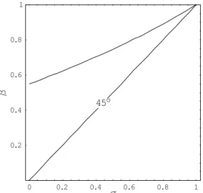
where F Ej is “Þxed effect” for country j, pjt is the relative price of capital in country j in year t, and²jt is noise term. β, as we explain immediately below, is monotonically related to σ, so once we get an estimate for β we can infer an estimate for σ. A plot of the monotonic relationship between σ andβ is shown in Figure 2 below.26
0 0.2 0.4 0.6 0.8 1 I
0.2 0.4 0.6 0.8 1
>
45o
Figure 2: Theoretical Mapping Connecting σ andβ
The economic relationship between σ and β is that σ is the elasticity of demand (for investment) when the timing of upgrades is Þxed, whereas β is the elasticity of demand
26Although there is no simple, closed-form expression linking σand β this functional dependence is
when the timing of upgrades is a choice variable.27 Because of the extra ßexibility, the
demand with timing is more elastic than the demand without timing, i.e., β is bigger than σ, which is seen by inspecting Figure 2.28
A word of caution is in order before we report our estimation results. When (23) is transformed into (24) we don’t actually get a log-linear relationship (the reason is that p
affects T in a non log-linear way). Nonetheless, if we Þx a value for σ and plot the true relationship between log i and log p, the curve we get is ‘nearly’ linear, and its slope is in one-to-one correspondence withσ. Thus, we proceed with the log-linear approximation (24) as our econometric speciÞcation.
7.2
D at a and Est im at ion
Using SH, we constructed a panel data-set for the period 1960 - 1985. The relative price of capital in this panel is the ratio between the price level of investment, SH variable PI, and the price level of consumption, SH variable PC. The investment in this panel is real gross domestic investment at 1985 international prices. This is the same panel that Restuccia and Urrutia (2001) constructed. For details, see the Statistical Appendix of their paper.
Regressing (24) by OLS, we got 0.57 for β. On the other hand, regressing (24) from the same panel - on the assumption that theÞxed effect is constant across countries, F Ej =F E - we got 1.09 for β. The reason for this difference is that p is negatively correlated with
B. Because of that, a cross-section estimation of (23), without controlling for variation in
B, biasesβ upwards, making it appear as though the production function is Cobb-Douglas, β = σ = 1. The rest of this section reports the results of further econometric exercises, which conÞrm thatβ is indeed signiÞcantly <1.29
To conÞrm that β <1 weÞrst ran various other regressions. We tried OLS with random effects, weighted least-squares, instrumental-variable with lagged-price as the instrument, and instrumental-variable, weighted least-squares with lagged-price as the instrument. The estimated values of β for these regressions were 0.64,0.45,0.63, and 0.45, respectively.
Second, we dealt with the following measurement problem. It has been suggested (see
27β isthe same asσin a model without embodiment and, hence, without timing decisions. β is also the
same asσwhenσ= 1(and embodiment) because thenT is independent ofp.
28As an example, consider the Leontief production function,σ= 0. Then, the elasticity of demand without
timing decisions is0. On the other hand, the elasticity of demand with timing decisions is0.55.
Pritchett (2000)) that the investment data reported for the poorest/high-peconomies are way above their true investments.30 If this suggestion is true, that would bias the estimated value
of β downwards. To check for that possibility, we constructed another panel by omitting all African economies. The unweighted instrumental-variable estimation of the new panel produced 0.73 forβ. The other estimates, OLS, weighted OLS, and weighted IV estimation produced 0.56,0.40, and 0.47, respectively. Thus, the estimated β from the restricted panel did not reverse the conclusion that β is less than 1.31
A third problem we addressed relates to using panel-data as opposed to cross-section data. A potential problem with panel-data is that it is difficult to distinguish between short-run (business-cycle type ßuctuations) and long-run movements. Since what we are trying to estimate is the long-run demand for investment, we smoothed the data by constructing Hodrick-Prescott (HP) Þltered data. The resulting OLS and weighted OLS estimates were 0.73 and0.63. The fact that the estimated β, which reßects price elasticity, increases when we go from the original data to the smoothed data is no surprise: as we smooth data, we go from short-run to long-run demand, so the price elasticity is expected to increase.
An important by-product of this smoothing exercise is that it shows we have enough variability in the data - in the time dimension - in order to estimate β. Indeed, if there were not enough variability we would have gotten smaller, not bigger, estimates for β. Overall, our results suggest that β is somewhere in the range [0.45,0.75]; it is deÞnitely less than 1.
Given these results and using the monotonic transformation betweenβ andσ, see Figure 2, weÞnd thatσ is somewhere in the range[0,0.4]. For the rest of this paper we pickσ= 0.4 which correspond to the OLS HP Þltered-data estimate of β.32
For this value of σ the calibrated value of α is 0.95, and of B, 0.27.
30Because the share of sector investments in total investment is high, and because data on
public-sector investments is exaggerated.
31We experimented with alternative ways of working with the data, including running different regressions
for different regions of the world. These experimentations did not alter ourÞnding. See our working paper.
32Further evidence corraborating our Þndings is found in Yuhn (1991). That paper surveys works that
estimate the elasticity of substitution for the U.S., and reports values between 0.078 and 0.763. See his discussion on page 343 and thereafter.
8
Quant it at ive Exer cises
In this section, we examine to what extent distortions account for income inequality across nations. The way we approach this issue here is that we “shut down” TFP and educational differences and ask how much income inequality can be explained by differences in distortions alone. The thought experiment therefore is to consider the whole world as having access to the same technology, and quantify the impact of bad economic policies (or other institutional and cultural features) that raise the cost of adopting new technology.33 We refer to this
exercise as “model simulation.”
We also examine how the answer to this quantitative exercise hinges on particular fea-tures of our model, which distinguish it from other models. In particular, we examine the sensitivity of our Þndings to the embodiment hypothesis.
8.1
Simulat ing t he m odel
We feed varying values ofpinto the (U.S.) calibrated version of the model and read offwhat effect this has on per-capita income. In doing so we hold the educational level h and the total factor productivity B constant, so as to isolate the effect of distortions.
We use the following procedure. The Þrst equation of system (20) gives us per-capita income (at t = 0) as a function of all parameters:
Beφ(h)
1−α
1−α ³
p
αBD(r+δ,T)
´1−σ
σ
σ−1
D(g+δ, T)
T .
Plugging calibrated and observed values, other thanp, into this expression we get a function, call ity(p), showing how per-capita income depends on distortions. We plot this function as the lower curve of Figure 3.
33A recent paper by Djankovet al. (2000) conducts an empirical comparison between countries regarding
0 1 2 3 4 5 6 7
p
0.2 0.4 0.6 0.8 1
y
y
S
U
Standard
Embodied
Figure 3
The most apparent feature of Figure 3 is that the lower curve spans a large range of incomes as p varies over a “reasonable domain.” In particular, if 1 ≤ p ≤ 5, which is the observed domain of prices in the SH data-set,34 then 0< y <1. Sinceyis income relative to
U.S. income, the theory explains the full range of observed income ratios. This is, of course, a very limited explanation because we are ignoring the roles ofB andh(which we discuss in Section 10). Nonetheless, the theory we put forward here already does much better than the “standard” model with disembodied technological progress and an aggregate, Cobb-Douglas production function; consult Lucas (1988) and Mankiw (1995) for how the standard model is used to assess development facts, and Chari et al. (1997) for a recent application. Indeed, if we do a similar calibration-estimation exercise for the latter (see next subsection) we get the higher curve in Figure 3.
Visual inspection reveals that the higher curve isßatter and, consequently, spans a much smaller range of incomes than the lower curve. The reason for that is that, under embodiment and σ < 1, the capital-elasticity of output increases when k decreases (and hence when
p increases), which magniÞes the effect of distortions, compared with disembodiment and σ = 1.
An extreme form of this is the possibility of a “poverty-trap;” i.e., that per-capita income
34From SH we computed5.1 = PPpi
pi, where the numerator is the 20 lowest-pcountries and the denominator
is zero. A poverty-trap might occur with σ = 0.4 but not with σ = 1. Indeed, whenever σ < 1, the marginal product of capital at K = 0 is Þnite, whereas when σ = 1, the same marginal product is inÞnite (the celebrated Inada condition). Thus, as p goes up, a point comes where an economy with σ < 1 stops upgrading its capital altogether, and becomes poverty-trapped. On the other hand, an economy withσ = 1 (orσ >1) always upgrades its capital - no matter how high p is; such an economy is never poverty-trapped.
8.2
Embodied ver sus D isemb odied Technological Pr ogr ess
Next let us compare - in greater detail - our model of embodied technological progress to the standard model of disembodied technological progress. Our point of departure from the standard model is two-fold. First, we consider embodied technological progress. Second, we consider individual production functions withσ= 0.4, whereas the standard model considers an aggregate, Cobb-Douglas production function withσ= 1. This raises the natural question why our model performs better. Is it the embodiment hypothesis? Or, is it the elasticity of substitution?
To address that question we do the following exercise. We construct the balanced growth-path of the disembodied model with a C.E.S. aggregate production function, whose elasticity of substitution is β. Then, we calibrate this model to U.S. data and estimate β, using the SH data-set. The estimated β is β = 0.7.35 These steps are perfectly analogous to those we
performed above; details are found in our working paper. Once we have these calibration and estimation results we construct the same y(p)functions for the disembodied model with β = 0.7and withβ = 1, and superimpose them on our, embodiedy(p)function withσ = 0.4. The result is shown in Figure 4.
As Figure 4 shows, going from β = 1 to β = 0.7 (i.e., keeping disembodiment, but using a different elasticity of substitution) already represents an improvement. However, going from disembodiment (with β = 0.7) to embodiment (with σ = 0.4) produces a far bigger improvement. Quantitatively, therefore, embodiment plays a more signiÞcant role in explaining income inequality.
0 2.5 5 7.5 10 12.5 15 p
0.2 0.4 0.6 0.8 1
y
Disembodied
s=1.0
Disembodied 0.7 Embodied
0.4
Figure 4
Another aspect of the model that this exercise points to is the following. Our model with individual production functions and embodied technological progress accommodate two features. On the one hand, the model gives rise to an aggregate demand for investment, which, when we estimate it, gives an elasticity of demand with respect to price of 0.73. On the other hand, the model features an individual production function with elasticity of substitution of 0.4, which, when we simulate it, produces poverty-traps with reasonable distortions, e.g., p= 5. By contrast, if one were to work with a disembodied model, one can either assume β = 0.4, get poverty-traps, but work with the wrong elasticity of demand for investment, or, one can assumeβ = 0.73, which corresponds to the right elasticity of demand for investments, but does not generate poverty-traps under reasonable distortions. Under disembodiment, it is impossible to get both a realistic elasticity of demand and poverty-traps for reasonable distortions. The advantage of our model is that it disentangles the price elasticity of investment from the elasticity of substitution (of the individual production function) and is thereby able to capture both features.
8.3
G r owt h M ir acles
human capital accumulation, as opposed to changes in total factor productivity.36 Young’s
Þndings are easier to reconcile with our model than with the standard model, as the following computation suggests. Consider the y(p) function that our theory cranks out evaluated at the price p = 4. This hypothetical price is taken to represent a highly distorted economy, which the East-Asian tigers are said to have been in the 50’s. Consider a change in economic policy that removes these distortions, resulting in p = 1. Then, as Figure 3 shows, we encounter a phenomenal growth experience - per-capita income increases Þve-fold, which, if we consider the time period 1960-1990, amounts to a compounded 9% annual growth-rate. On the other hand, if we consider the standard model, as calibrated in Section 8.2, per-capita income merely doubles, amounting to 3% per-year growth rate. So if B remained constant over the period 1960-1990, then our theory reproduces the actual growth experience of the East-Asian tigers much better than the standard model.
Although suggestive, one should be a bit cautious with this exercise. This is because the y(p) curve connects steady states rather than showing a transition path between steady states. The next natural step in this line of research, which goes beyond the scope of the present paper, is to investigate explicitly transitory dynamic and what it implies about growth-rates when p goes down.
8.4
Cont r ast ing t he Simulat ed M odel wit h D at a
Another way of contrasting our model with (cross section) data is the following. We can ask how actual data compares to our simulated y(p) curve. That curve is derived on the assumption that h and B are constant, and equal to their U.S. levels, whereas, in the real world, h and B are (obviously) not constant. To partially account for cross-country variation in (h, B), we use the following procedure. Using Hall and Jones (1999) (HJ) data we construct the ratios (country j’s income)/(country j’s educational factor)*(U.S. income), where per-capita incomes yj, which are net of the mineral sector output, and educational factorseφ(hj) come from HJ. This accounts for theh, but not for theB, variation, which we
are not able to observe. Then, we pair up these ratios with thepj’s reported by SH, and put these pairs on a two-dimensional diagram. On the same diagram we superimpose the y(p) function calculated above. The result is shown below as Figure 5.
36As far as total factor productivity, B, if anything, theB of the East-Asian tigers is below the average
0 1 2 3 4 5 6
p
0.2 0.4 0.6 0.8 1 1.2 1.4
e
m
o
c
n
I
n
o
i
t
a
c
u
d
E
Embodied
SAU
EGY TTO
SUR
s=0.4
Figure 5
As this Figure shows, most scatter points lie below the y(p) curve. We take this fact to imply that the U.S. economy operates at a high efficiency; i.e., has a higher TFP than most countries. Indeed, the scatter points in this diagram are created without correcting for different countries having different B’s. Hence, whenever a country has a smaller B than the U.S., its scatter point lies below y(p), which is what the Figure shows.37
9
M odel Pr edict ions
In Section 8 we examined how the model works as a theory explaining income inequality. In this section we discuss various other predictions along which the model can be tested. The methodology here is similar to that of Section 8. We Þx h and B while varying p, and ask what effect this has on various economic statistics. We also compare the predictions we get in this way to those we get when the elasticity of substitution is 1 (instead of0.4).38
37We tried to account for theB’s by taking the impliedB from the regressions in Section 7. However, the
B for some African countries is excessively high because the model does not work well for large p’s. As a result of this the scatter diagram became very dispersed.
A natural solution to this is to throw out some countries whosepand, hence, impliedB is high. However, it is not obvious which criterion to use when deciding which observations are to be thrown out. Because of that we treatB as a residual in this exercise.
38This comparison is closely related to a comprison with the standard model, since, when σ = 1, the
Many of our model’s predictions hinge on the mechanics of upgrading and how it relates to distortions. In particular, each Þrm periodically upgrades its technology. The length of the upgrading period varies positively withp; namely, a higher pimplies a Þrm will hold on to its technology for a longer time (see Proposition 2). This creates a “window effect” where more distorted economies hold more antiquated and, hence, lower-quality capital. Related to this, the price of old capital decays more slowly the more distorted the economy is (see Figure 1). These two effects create a “paradoxical” valuation of capital stocks, where poor countries appear to have a large aggregate capital stock.39 Many of the patterns we report
below are due to these features of the model.
• The Investment-Capital ratio. This ratio is decreasing in p, and quantitatively the decrease is quite steep; see Figure 6.1. As suggested, the logic behind this is that capital goods are held for a longer time and their prices decline at a lower rate as p
increases. This increases the market value of the capital stock, which decreases the investment-capital ratio. On the other hand, for σ = 1 this ratio is constant in p
(because the holding period is independent of p).
Another prediction that this exercise brings out is that economic depreciation is large relative to the sum of physical and technological depreciations. Indeed, as p increases the height of the curve converges toδ+g, which is the sum of physical and technological depreciations. Everywhere else the curve is higher and, for “reasonable” values of p, it is signiÞcantly higher.
• The Capital-Output Ratio. To make this ratio comparable across countries, we divide it by p. For σ = 1, this curve is downward sloping, with unit elasticity (see Figure 6.2). For σ < 1, the curve declines at a lower rate and may even bend upwards and increase. For our σ = 0.4, the curve is, in fact, U-shaped. The reason for this is that as p increases, output always decreases. However, the market value of capital is subject to two opposing effects. The quantity of capital installed always decreases (see Proposition 2), which makes the capital stock smaller. On the other hand, capital is held for a longer time and its price declines more slowly. This makes the market value of capital bigger. Which of these effects dominates depends on the value of σ.
39This is due to the fact that, at a given point in time, more capital goods are “ßoating around” and that