Comments Requested.
Technical Change and Fa ctor Shares
by
John J. Seater
Economics Department North Carolina State University
Raleigh, NC 27612
Abstract
The implications of technical change that directly alters factor shares are examined. Such change can lower the income of some factors of production even when it raises total output, thus offering a possible explanation for episodes of social conflict such as the Luddite uprisings in
19th century England and the recent divergence in the U. S. between wages for skilled and
I. Introduction
This paper examines some implications of technical change that alters the relative shares
of output accruing to the factors of production. This type of technical change was studied
extensively in the first “golden age” of growth theory (after Solow-Swan to about 1980) but has
been largely ignored in most of the second golden age (the post-Romer literature on endogenous
growth theory), which generally treats technical change exclusively as an increase in total factor
productivity. For example, the usual quality ladder model of endogenous growth has an
aggregate production function of the form
where L is labor, the Xi are intermediate goods produced in other sectors, and the qi are indices of
the quality of the Xi. Technical change is captured by increases in the quality indices. The factor
shares " and 1-" are unchanged by quality improvements. In the real business cycle literature,
productivity shocks always take the form of changes in the total factor productivity coefficient in
front of the production function. Again, factor shares are assumed unchanged.
There are at least two reasons why share-neutral technical change seems likely to be the
exception rather than the rule. The first is the nature of the production function itself. A
production function is merely a mathematically convenient way to express the relation between
output and inputs. Technical change is by definition a change in that very relation. There seems
no reason whatsoever to assume a priori that such a change in the production function is
1
For example, in the CES production function
changes in either a or R alter factor shares.
neutral TFP coefficient generally alter factor shares.1
The second and more important reason for doubting share-neutrality of technical change
is that the data show systematic changes in factor shares over time, a fact that has been known for
several decades. Table 1, taken from Sato (1970), reports capital’s share in the private non-farm
sector of the US economy over the period 1909-1960. Figure 1 plots the data and shows quite
clearly that physical capital’s share of output fluctuated considerably from year to year and
followed an overall downward trend over the entire period. Capital’s share has a maximum of
0.397 and a minimum of 0.301, nearly a 33 percent increase from the min to the max, a large
swing for a number that goes into the exponent of the Cobb-Douglas production function. The
time trend is statistically significant. Regressing the log of capital’s share on time yields
where " is capital’s share and numbers in parentheses are standard errors. The p-value of time’s
coefficient is 0.0085. In addition, there is a great deal of fluctuation about the trend, as indicated
by the adjusted R-squared value of only 0.113. These data belie the oft-heard assertion that
“capital’s share is roughly constant at about thirty percent”; capital’s share quite clearly is not
constant over either the short run or the long run. Sato and Hoffman (1968) present data for
Japan over the period 1930-1960. The regression coefficient of capital’s share on the log of time
is -0.039 with a standard error of 0.014 (p-value of 0.0094) and an adjusted R-squared of 0.189.
non-2
Katz and Murphy (1992), among others, document that the wages of skilled workers have increased relative to those of unskilled workers. Bound and Johnson (1995) show that the supply of skilled workers also has increased relative to that of unskilled workers, thus
establishing that skilled workers’ income share has risen relative to that of unskilled workers.
3
An enormous early literature examined the origins and extent of biased technical progress, beginning with Kennedy (1964). The recent shift in relative wages for skilled and unskilled labor in the U. S. has revived research into biased change. See Caselli (1999) and Acemoglu (2000) for two recent theoretical investigations. Some investigators, such as Borjas and Ramey (1994) and Dinopoulos, Syropoulos, and Xu (1999), argue that changes in the pattern of trade explain the relative wage shift between skilled and unskilled workers. Although
possibly true, that explanation begs the question of why trade patterns have shifted. Presumably, the ultimate explanation is changes in technology, unless one wants to invoke changes in tastes. Baldwin and Cain (1997), Harrigan and Balaban (1999), and Bartel and Sicherman (1999) are among those providing evidence that technical change explains the relative wage shift. production workers in the U. S. all have trends and variation about those trends over the more
recent period 1959-91. Blanchard (1997, 1998) finds that capital’s share in Europe has been
similarly variable, falling before the mid-1980s and then rising sharply thereafter in many
European countries. We have more than just simple statistics showing changes in capital’s share.
A wide range of formal econometric investigations of biased technical progress finds capital and
labor shares changing over time. Sato and Kendrick (1963), David and Klundert (1965), Sato
(1970), Sato and Hoffman (1968), to name a few, do so by estimating production functions;
Binswanger (1974), Stevenson (1980), and Kumbhakar and Lozano-Vivas (2000) reach the same
conclusions by estimating cost functions. Finally, the past thirty years or so in the US have seen
a large increase in the share of output going to skilled labor at the expense of the share going to
unskilled labor (Bound and Johnson, 1995).2
So the income shares of subsets of the labor force
also have shown movements over time. Factor shares are not constant, even approximately.
The present paper takes biased technical change as given and analyzes some of its
macroeconomic implications without explaining where such change comes from.3
results are obtained. The theory offers an explanation for the social conflict between owners of
capital and labor, such as the famous Luddite uprisings in England in the early 19th century. It
also offers an explanation for why some countries, notably underdeveloped ones, do not adopt
the latest technological breakthroughs but continue to use apparently outdated production
methods. A large fraction of endogenous growth models are called into question by the
implications of technical change that alters factor shares. Finally, it is shown that total factor
productivity can fall (rise) as the result of technical change that raises (lowers) aggregate output,
suggesting that total factor productivity is a rather poor indicator of technical progress.
II. Two Factors of Production
We start with the case of only two factors of production, capital and labor. We consider
later a three factor model that separates physical and human capital. The two factor case is much
easier analytically, permitting detailed dynamic analysis that cannot be done in the three factor
framework. Moreover, the essence of most macroeconomics is aggregation, so the two factor
model with capital of all forms treated as a single entity may have some methodological appeal,
at least to those tending to be lumpers rather than splitters. In all that we do, production is
Cobb-Douglas:
(1)
where Y is output, K is capital, L is labor, A is total factor productivity, and " is capital’s share.
4
A number of early studies (e.g., Sato, 1970) present evidence that the elasticity of substitution is less than one, which would rule out the Cobb-Douglas function. However, those studies all fail to distinguish between raw labor time and human capital, attributing all labor income to hours. If human capital were lumped with physical capital rather than with man-hours, the estimated elasticity of substitution would rise substantially. It thus is not clear that the Cobb-Douglas function is ruled out.
(2)
(3)
The use of Cobb-Douglas production to discuss variable factor shares may seem
surprising; the usual assumption with Cobb-Douglas is that shares are constant. Samuelson
(1965), for example, begins his discussion of induced innovation with the Cobb-Douglas case
and imposes without discussion the restriction that factor shares are constant. However, Sato and
Beckmann (1968) propose fourteen definitions of neutral technical progress, three of which
permit Cobb-Douglas production with changing factor shares. They then do some empirical
work with data from Germany, Japan, and the United States and show that such a production
function is acceptable for all three countries and for Japan even offers the best fit of the various
types considered. So the use of Cobb-Douglas production with changing factor shares in the
following theoretical discussion is not at all unreasonable.4
II.A. Simple Technical Change With Fixed K and L.
We begin by examining the situation where a technical invention alters only the factor
shares, leaving total factor productivity A the same. We also assume for now that both capital
5
Results for the case where the invention reduces " are completely symmetric to those
discussed here.
Suppose an invention is discovered that alters "; for expository ease, suppose that the
invention raises ".5
Will the invention be adopted? To decide, we examine the effect of an
increase in " on the incomes of the total economy and the two factors of production. The
derivatives of Y, MPK, and MPL with respect to " are
(4)
(5)
(6)
We thus have four phases, depending on the value of ln(K/L)
which have the following characteristics:
I: 0 < MY/M", MMPK/M", MMPL/M"
II. MMPL/M" < 0 < MY/M", MMPK/M"
III. MY/M", MMPL/M" < 0 < MMPK/M"
IV. MY/M", MMPK/M", MMPL/M" < 0
each factor’s total income moves in the same direction as its marginal product.
The pre-invention values of " and K/L determine which phase the economy is in. A
large capital/labor ratio places the economy farther to the right on the phase line (i.e., in a lower
numbered phase), given an initial value of ". The initial value of " affects the positions of the
boundaries between phases I and II and between phases III and IV. An increase in the initial
value of " moves both boundaries to the right, reducing the size of phase III and increasing the
size of phase II (phases I and IV both remain infinite in size). The boundary between phases II
and III is anchored at zero and so does not depend on the initial value of ".
The intuition for why the economy’s phase depends on the capital/labor ratio is not
difficult. An increase in " increases the exponent of capital and reduces the exponent of labor in
the production function. If capital is relatively abundant, this shift in exponent magnitude from
labor to capital will raise output; if capital is relatively scarce, it will reduce output. A similar
intuition underlies the changes in factor incomes.
If the economy is in phase I, adopting the invention is Pareto optimal; the income of both
factors of production rises. Although labor’s share of output falls with the increase in ", total
income rises by more than enough to offset this effect, as shown by the increase in MPL and thus
labor income. Phase IV is the symmetric case, in which adoption reduces social welfare because
it would make everyone worse off.
Phases II and III are more difficult. In phase II, total output rises, capital’s income also
rises, but labor’s income falls. In phase III, only capital’s income rises; both total income and
labor’s income fall. Adoption is not Pareto optimal in either case. Adoption is net benefit
optimal in phase II and net benefit suboptimal in phase III because adoption raises total output in
with the representative agent model; Pareto optimality then coincides with net benefit optimality.
In that case, adoption is Pareto optimal if the economy is in phase II; it is Pareto suboptimal if
the economy is in phase III (at least for now; we will see that adoption can be socially optimal
even if the economy is in phase III once the economy’s dynamic response is taken into account).
A general conclusion that emerges is that technical change that alters only factor shares
will have increasingly broad social benefits the more abundant is the factor whose share
increases. In particular, for a given capital/labor ratio, this kind of technical change can raise
total output only if it favors the relatively abundant factor. As we will see below, this latter
implication does not necessarily hold if the capital/labor ratio can change in response to the
technical change or if the technical change alters total factor productivity as well as factor shares;
nonetheless, even in these more general settings, share-altering technical change tends to favor
the abundant factor. This tendency may help explain Berman’s (2000) recent finding from a
three-dimensional panel (industry, country, time) that, in the decade of the 1980s covered by the
panel, technical change was strongly biased against less-skilled workers and in favor of both
physical and human capital. If research and development is conducted largely by industries in
developed countries for the benefit of those same industries, it will tend to favor technical
advances that increase the income shares of the relatively abundant factors - that is, of physical
and human capital. We will return to this line of argument below, when we consider which
countries are likely to adopt a given type of technical change.
As interesting as the normative side of adoption is the positive side. It is clear that the
invention will be adopted if the economy is in phase I and will not be adopted in phase IV. The
economy’s competitive equilibrium can be obtained as the solution to a central planning
adopt in phase I. Consequently, the competitive equilibrium solution for an economy in phase I
must be adoption. Similarly, the planner would not adopt in phase IV because adoption makes
everyone worse off. The competitive equilibrium in phase IV therefore is not to adopt. If the
economy is in phase II or III, we cannot say whether adoption will occur. The outcome depends
on who makes the adoption decision. If owners of capital decide, then the invention will be
adopted if the economy is in either phase II or phase III because captial’s income is raised in both
cases. Similarly, if labor makes the decision, the invention may not be adopted in either phase II
or phase III because labor loses in either case. We thus have two interesting possibilities. First,
an invention that raises aggregate output may not be adopted because it is opposed by one of the
factors of production. Second, an invention that lowers aggregate output may be adopted
anyway because it is favored by one of the factors of production. Recall that in all this
discussion we are assuming the invention raises capital’s share ". Symmetric results obtain if
the invention raises labor’s share 1-" instead.
The first of the foregoing possibilities may explain the famous episode of the Luddites,
who sporadically destroyed textile machinery in various English towns over the period
1811-1816. The Luddites blamed the machines for the prevailing unemployment and low wages. The
Luddites are usually written off in the history books as misguided fanatics, but in fact they may
have been right about the cause of low wages, at least in their industries. If the textile machines
(or perhaps “new and improved” machines that replaced older ones) raised capital’s share, and if
England at the time was in phase II, then the introduction of the machines would have
simultaneously raised total output and capital income on the one hand and reduced labor’s
income on the other hand. Indeed, the Luddite uprisings occurred fairly early in the Industrial
A low capital/labor ratio could have put England in a phase below phase I and thus could have
created conditions favoring uprisings by the workers against technical change that raised
capital’s share. The subject merits further examination by economic historians. We will see a
similar phenomenon at work later when we introduce human capital and discuss a possible
explanation for the recent shift in income shares among low-skill and high-skill workers in the
United States.
The analysis also has an interesting implication for the adoption of new technology by
different countries. Suppose there are two countries, A and B, that use the same production
technology (i.e., the same production function) but have different capital/labor ratios, with
country A's ratio exceeding that of country B. Suppose also that the capital/labor ratios are such
that country A is in phase I (relatively abundant capital) and country B is in phase IV (relatively
scarce capital). An invention that raises " will be adopted by country A and will not be adopted
by country B. Once country A has adopted the invention, it no longer has the same production
technology as country B. The usual argument that all countries should have the same production
functions because technology is freely transferrable therefore may be incorrect, suggesting that
cross-country estimation and testing based on such an assumption may be misspecified.
Adoption of the invention alters the conditions that determine the desirability of
subsequent inventions. In the example just discussed, after country A adopts the invention, its
value of " is higher than before. This change moves the boundary between phases I and II to the
right, increasing the range of capital/labor values that fall in phase II and thus tending to move
6
This discussion recalls and is related to the concept of the technology frontier,
introduced by Kennedy (1964), subsequently discussed and expanded by Samuelson (1965) and others, and recently rediscovered by Caselli and Coleman (2000).
7
The mechanism here differs fundamentally from that discussed by Basu and Weil
(1998), even though the capital/labor ratio is central in both treatments. Basu and Weil assume a Cobb-Douglas production function with a fixed capital share but also assume that total factor productivity depends on the capital/labor ratio:
where y=Y/L is output per person and k=K/L is the capital/labor ratio. In addition, they assume that for each k there is a maximum possible value of A, denoted A*(k). In contrast, the present
treatment takes A as independent of k but allows capital’s share " to change over time.
inventions that raise ".6
However, as we will see below, the change in " brought about by
adoption also increases the steady state value of the capital/labor ratio, which puts country A
deeper in phase I. It therefore is unclear whether adoption moves country A away from or
toward the boundary between phases I and II.7
We return to this issue after we discuss the
economy’s dynamic response to the invention. Before we study system dynamics, we examine
mixed technical change, in which both total factor productivity A and capital’s share " are
altered by an invention.
II.B. Mixed Technical Change.
The previous discussion has been useful for explaining the effects of changes in factor
shares brought about by an invention. However, production functions are just convenient
mathematical representations of reality, and reality is very complex. One therefore should expect
that a real-world invention generally would alter all the parameters of the production function.
We can call this mixed technical change. In our simple Cobb-Douglas case, there are only two
parameters to consider: total factor productivity A and capital’s share ". We now examine the
effects of mixed technical change that alters both of these parameters.
(7)
(8)
(9)
Denote dA + A ln (K/L)d" by Z. Then the three foregoing conditions can be written as
(10)
(11)
(12)
We can write a chain inequality showing the relation among the three terms on the far right sides
of the foregoing expressions:
(13)
discussion by restricting attention to the case where d" > 0. We then obtain the same results as
in the previous section with only slight modification. There are four phases the economy can be
in, depending on the value of Z and as shown in the following diagram:
The discussion of when adoption will be socially optimal and when it will occur in competitive
equilibrium parallels that of the previous section, with the capital/labor ratio replaced by Z. We
therefore need not pursue that discussion in any further detail here, except to note that technical
change generally will involve changes in both A and " so that, in contrast to the analysis of the
preceding section, it no longer is true that only technical change that favors the abundant factor
will raise total output Y.
This analysis suggests that total factor productivity A may not be a reliable indicator of
technical progress. It is possible for Y, MPK, and MPL all to increase in response to a technical
change even though the change reduces total factor productivity. For Y, MPK, and MPL to
increase in response to the technical change, the economy must be in phase I. The required
condition is
(14)
Recall that for this discussion we are assuming d" > 0, so the economy can be in phase I and still
have dA negative if the quantity in brackets is negative, that is, if ln(K/L) > 1/(1-"). We thus
income but is nonetheless associated with a decline in total factor productivity. Symmetrically,
we could have situations in which Y, MPK, and MPL all fall even though A rises. The
usefulness of total factor productivity as a measure of technical progress thus is questionable.
II.C. Dynamics.
We now examine the dynamic response of the economy to an episode of technical
progress that alters factor shares. To make the analysis possible, we must assume the existence
of a representative agent so that we can posit and solve a social planning problem. We also make
three simplifying assumptions. First, labor supply L is taken as fixed throughout the discussion.
Labor supply can vary either because the population grows or because hours per worker change.
Allowing exogenous population growth adds nothing to the analysis, so we assume population
growth is zero. Allowing hours of labor to be set as part of the optimization complicates the
analysis in the usual way without providing any useful insights, so we suppose that everyone
works a fixed amount. We thus are in the framework of the standard Cass growth model with
population growth set to zero. Second, we assume dFK > 0 because otherwise the economy
would be in Phase IV, so that the invention would benefit no one and would not be adopted.
Assuming dFK > 0 is equivalent to assuming that ln(K/L) > -1/" (see section II.A above). Third,
we suppose through most of the discussion that only " is changed with total factor productivity A
unaffected. As we already have seen, the conditions for the economy to be in its various phases
are very similar for the cases when A does and does not change. So for simplicity, we hold A
fixed for most of the analysis; at the end, we examine briefly the effect of allowing it to change.
8
The specification of the budget constraint is correct only for interior solutions, that is, for solutions where 0 < C < F(K, L). We ignore corner solutions throughout because they add nothing to the analysis.
subject to the aggregate budget constraint:8
(15)
where U is a concave utility function, C is consumption, D is the rate of time preference, and * is
the depreciation rate. The current value Hamiltonian is
(16)
where R is the costate variable. The necessary conditions are
(17)
(18)
(19)
(20)
(21)
We obtain the equilibrium loci from these conditions in the usual way and so do not dwell on the
details of their derivation. The equilibrium locus for capital (dK/dt = 0) is given by
(22)
where C(R), obtained from the first-order condition (19), is the function relating consumption to
dK/dt=0 locus is
(23)
The equilibrium locus for the costate variable (dR/dt = 0) is given by
(24)
The dR/dt=0 locus is vertical at K*. We thus have the usual phase diagram, shown in Figure 2.
Note that K* is the steady state stock of capital.
Suppose now that an invention is discovered that raises " and leaves A unchanged.
Because FK > 0 (by assumption), it is immediately apparent from (24) that K* increases, causing
the dR/dt=0 locus to shift to the right. Whether the dK/dt=0 locus shifts up or down depends on
whether the economy is initially in phase II or III, which depends on the sign of MY/M". If
MY/M" > 0, the economy begins in phase II, and it is straightforward to see from (22) that the
dK/dt=0 locus shifts down. We have the situation shown in Figure 3. The steady state moves
from point E0 to point E1, at which the capital stock is higher and R is lower (and therefore
consumption C is higher) than originally. The exact dynamic adjustment path that will be taken
to the new steady state is unclear. It could be that, immediately after the invention is adopted, R
jumps up © jumps down) and the upper path PU is followed, or it could be that R jumps down ©
jumps up) and the lower path PL is followed. Which path is taken depends on the magnitudes of
the production and utility function derivatives and of the other system parameters.
optimal. To see this, first suppose path PL is the optimal adjustment path. Along that path,
consumption and therefore utility is higher at all times than if the invention is not adopted and
the economy remains at point E0. Unambiguously, adoption is optimal. Now suppose that path
PU is the optimal path. Recall that optimality here is a conditional notion; if the invention is
adopted, then the optimal path to follow is PU. Along this path, initial consumption and therefore
utility is lower with adoption than without it. It therefore is not immediately clear that adoption
is optimal. However, notice that a path like PL always is feasible even if not optimal. The
impact effect of the invention is to raise output, by assumption. Some of that increase in output
could be used to raise consumption immediately and the rest used to increase the capital stock K.
The increase in K would increase output further as time passed, allowing ever more
consumption. Path PL thus dominates the alternative of not adopting the invention and remaining
at point E0. In the case under consideration, however, path PL is itself dominated by path PU, so
adoption is optimal a fortiori.
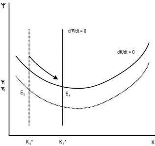
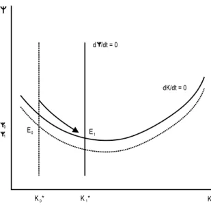
Suppose now that the economy initially is in phase III, where MY/M" < 0. In that case,
the dK/dt=0 locus shift up, and we have the situation shown in Figures 4 and 5. Figure 4 is
drawn with the new steady state value R1 of the costate variable above the initial value R0. The
value of R is above R0 along any possible dynamic adjustment path, meaning that consumption
and thus utility are always lower than they were before adoption. Adoption is unambiguously
suboptimal. An interesting possibility, however, is shown in Figure 5, where R1 is below R0,
implying that consumption and utility eventually exceed their pre-adoption levels. If the
eventual increase in utility is great enough to dominate the decline early on the adjustment path,
On the right side, we can use (19) to solve for R0 in terms of A, D, *, L, and "0 (the value of "
before adoption of the invention). However, on the left side, we must know the entire path of R,
which requires an explicit forms for the utility function U. Even then, an analytic solution
usually is not possible. In principle, though, the path of R on the left side will be determined by
A, D, *, 8, "0, "1 (the value of " after adoption of the invention), and the levels and derivatives
of U and F. In addition to satisfying the foregoing inequality, the parameters A, D, * and "0
must have values that satisfy the two inequalities required for the economy to be in phase III:
where we have used (24) to eliminate K/L in passing from the first line to the second. We thus
have a total of three inequalities to satisfy and many more than three parameters to vary. In
general, we should be able to find combinations that satisfy all three inequalities, thus leading to
the conclusion that adoption of the invention can be socially optimal even though it initially
reduces output, consumption, and utility.
III. Three Factors of Production
production function. Many of the results are straightforward generalizations of those obtained
for the two-factor model, but the three-factor model still is worth examining because it has
important implications for the recent divergence between incomes of skilled and unskilled labor
and also for the failure of many underdeveloped economies to adopt technological advances, an
issue already touched on above.
The production function now is a three-factor Cobb-Douglas:
(25)
where H is human capital. With human capital entering as a separate factor of production, we
now should interpret L as (man hours of) raw or unskilled labor. The marginal products of the
three factors are
(26)
(27)
(28)
III.A. Simple Technical Change with K, H, and L Fixed.
As in the two-factor case, we start by examining the effect of a technical change while
holding all factors of production fixed. We thus are examining the impact effect of the change.
With an additional factor of production, we also have an additional factor share to consider. The
previously; to keep the discussion tractable, and to concentrate on the most interesting case, we
restrict attention to a technical change that alters the relative shares of human capital and
unskilled labor while leaving physical capital’s share unchanged. In particular, we suppose the
change raises human capital’s share $, lowers unskilled labor’s share 1-"-$, and leaves physical
capital’s share " unchanged. For now, we also simplify the discussion by supposing total factor
productivity A is unchanged. We thus have a situation that parallels that of section II.A above,
with human capital taking the place of physical capital in the discussion.
The economy can be in one of four possible phases, determined as in section II.A by the
signs of the effects of the technical change on the level of output and the incomes of the three
factors of production. The derivatives of Y, MPK, MPH, and MPL and their signs are
(29)
(30)
(31)
(32)
and have the following characteristics:
I: 0 < MY/M$, MMPK/M$, MMPH/M$, MMPL/M$
II. MMPL/M$ < 0 < MY/M$, MMPK/M$, MMPH/M$
III. MY/M$, MMPK/M$, MMPL/M$ < 0 < MMPH/M$
IV. MY/M$, MMPK/M$, MMPH/M$, MMPL/M$ < 0
Which phase the economy is in depends on the pre-invention values of ", $, and ln(H/L).
The adoption results are the same as in section II.A, so we need dwell on the details.
Adoption always is optimal and occurs in phase I, adoption never is optimal and never occurs in
phase IV, and adoption may or may not be optimal and may or may not occur in phases II and
III. What is worth spending some time discussing are the implications of these results for two
current events.
III.A.1. Unskilled labor’s income share.
It has been widely noted that in the United States over the last thirty years or so the real
income of unskilled labor has been stagnant while total income and the incomes of physical
capital and especially human capital (skilled labor) all have risen. This event is regarded by at
least some people as evidence of a breakdown in “the system” that has left unskilled workers
behind and that must be corrected by some sort of government intervention. The foregoing
results suggest that existence of the event in question is not compelling evidence of a defect in
the workings of the economy. A technical change that raises the income share of skilled labor
check which phase the economy is in simply by examining the relation between ln(H/L) on the
one hand and the share parameters " and $ on the other. In practice, this is difficult to do
because data on human capital H are sketchy at best.
Of course, real-world technical advances generally will be more complex than that
discussed in this section; in particular, we would expect total factor productivity A and probably
physical capital’s share " to change in most cases. Indeed, the data show an upward trend in A
and a downward trend in ". We have seen, however, that allowing A to change does not alter the
general character of the results. Allowing " and $ to change simultaneously complicates the
results but again does not change the main conclusion that it is quite possible that a technical
advance can reduce the income of unskilled labor even though it raises total output and the
incomes of other factors of production.
III.A.2. Adoption of new technology by underdeveloped economies.
We already have seen in section II.A that countries with different capital/labor ratios may
make different adoption decisions regarding a technical advance even if they have the same
technology at the time the advance is made. A similar result emerges here but now seems much
more likely to occur. Suppose countries A and B have the same technology but different human
capital/labor ratios, with A having the higher value of H/L. An invention that raises $ is more
likely to be beneficial to country A than to country B and so more likely to be adopted by A than
by B. Recent experience in the United States, just discussed in section III.A.1, suggests that
important recent technical advances have raised $. We therefore should expect to see countries
with higher values of H/L adopting those advances. Although we do not know how to measure
H exactly, it seems likely that levels of education should have a positive correlation with H. If
9
Education plays a decisive role in Caselli and Coleman’s (forthcoming) discussion of structural transformation and regional convergence in the US economy.
they are the countries with relatively high levels of education. Such recent technological
advances may not make poor countries any poorer, but they do make the rich countries richer and
increase the amount of income inequality across countries. Again, this outcome is not in any
way due to a defect in “the system” but merely a consequence of the relative factor endowments
of different countries. It does, however, emphasize the importance of education and government
policies that encourage it.9 It therefore may explain why some countries seem stuck in a state of
underdevelopment. Basic education is not something that firms typically will invest in, simply
because its general nature prevents firms from capturing the return to any investment they make
in it. Rather, basic education must be undertaken by individuals themselves. In most countries,
government provides or subsidizes basic education. If the government does this job badly, then
it may condemn its economy to the use of backward technology, guaranteeing that the economy
remains poor. This sort of failure may even instigate a vicious circle. In the foregoing
discussion, education may bring little reward if the available technology is suited for a low level
of education. People therefore may be discouraged from acquiring education in the first place,
thus guaranteeing that the technology will remain backward and continue to not reward
education. In addition, low levels of education hold down the marginal product of physical
capital, making business fixed investment unattractive. We will further pursue this issue in
section III.C below.
This last prediction resembles Caselli and Coleman’s (2000) empirical finding that
countries with a relative abundance of unskilled labor are relatively inefficient at using skilled
in the following variant of the CES production function:
Unfortunately, the limit of this function as F and D go to zero is not Cobb-Douglas but rather
The factor efficiencies do not become factor shares (all of which are 1 in this case) when the
elasticity of substitution goes to one, as they do for the standard CES function
Thus Caselli and Coleman’s estimates of factor efficiencies cannot be applied to the
Cobb-Douglas functions used throughout the present analysis; nonetheless, they are consistent with the
predictions obtained above.
III.B. Mixed Technical Change.
Allowing total factor productivity A to change leads to the same conclusions as in section
II.B above. The main effect is to change the expressions that define the boundaries of the four
phases. The details are left to the reader.
III.C. International Capital Flows in a Dynamic Model.
Because there now are two state variables, K and H, a full dynamic analysis like that
performed for the two-factor model is not be feasible. It is possible, however, to work out the
steady state solutions. The results for a closed economy are not much different from what was
obtained in section II.C above. In contrast, the results for in a model with international capital
flows provides interesting insights into economic development. Discussion will be brief with
mathematical details relegated to the Appendix.
developed and exports physical capital to country E, which for simplicity is assumed to produce
no capital of its own. All markets in both countries are competitive. The two countries produce
the same final good with the aggregate Cobb-Douglas production function
where i = D or E. Each country takes what the other country does as given.
Country D’s planning problem is to maximize the representative agent’s utility over
domestic consumption CD , investment IE in capital located abroad, and investment IH in domestic
human capital
(33)
subject to the dynamic equations
(34)
(35)
(36)
The second term on the right side of the second line in (34) is income from capital located in
country E, equal to the marginal product of KE multiplied by KE itself. Solving this problem with
the maximum principle leads to the following steady state solution for KE:
(37)
chosen by country E.
Country E’s problem is simpler because it does not build physical capital either at home
or abroad. It therefore chooses only its consumption CE to maximize representative agent utility:
(38)
subject to
where the first term on the right side is GDP less the income from capital, all of which goes to
country D. The steady state value for HE is
(39)
Note that HE, which is chosen by country E, depends positively on the value of KE, which is
chosen by country E.
Equations (37) and (39) can be solved simultaneously for the Nash equilibrium values in
terms of the underlying parameters of the two economies. Those values then can be substituted
into country E’s production function to obtain the equilibrium solution for output. What interests
us here is the response of country E to an increase in $E. The solution for output in country E,
conditional on country D’s choice of KE, is obtained by substituting (39) into country E’s
(40)
The decision by Country E’s planner on whether to adopt a technical change that increases
human capital’s share at the expense of unskilled labor, while leaving physical capital’s share
unchanged, depends on the sign of the derivative of output with respect to $E, which determines
whether adoption raises or lowers total output. The derivative is
(41)
The sign of the first term on the right side is ambiguous in general. The second term on the right
side, however, is positive or negative as KE is greater or less than LE. Therefore, the higher the
capital/labor ratio, the more likely country E is to adopt a technical change that raises $E.
Intuitively, adoption is increasingly beneficial the higher is the level of human capital HE, but the
level of HE depends positively on KE. When a new technology arises that favors human capital,
country E is less likely to adopt if it is relatively scarce in human capital. It is likely to be scarce
in human capital if it is scarce in foreign investment. Foreign investment is likely to be low if
human capital is low, as can be seen from the solution for KE given by (37). But human capital is
likely to be low if $E is low, because human capital’s marginal product (return to human capital)
depends positively on $E. This is the vicious circle referred to earlier: low foreign investment
holds down human capital, which makes adoption of technical changes favoring human capital
10
See Barro and Sala-i-Martin, Chapter 4.
seems especially relevant in recent years, when, judging from the U. S. experience, there have
been substantial technical advances favoring human capital at the expense of unskilled labor.
These advances may be of little value to countries with low levels of human capital, which may
remain stuck in a poverty trap relative to the developed nations.
IV. Share Changes in Endogenous Growth Models
To this point, we have considered only models in which growth is exogenous (and, to
keep matters simple, have assumed there was no exogenous growth). We now look at a few
examples of endogenous growth models and study the effect of technical change that alters factor
shares. The general result is that the economy’s growth rate changes, with the direction of
change depending on the magnitudes of some of the economy’s parameters. However, a serious
question also arises concerning the plausibility of many endogenous growth models.
IV.A. AK-Type Models.
The simplest AK model, with the production function
(42)
has only one factor of production with a fixed share of one, so technical change that alters factor
shares is ruled out by implicit assumption. Slightly more elaborate AK-type models admit such
change, however. In particular, consider the model of learning-by-doing with knowledge
spillovers.10
We suppose the production function is
(43)
11
This form has been shown by King, Plosser, and Rebelo (1988) to be necessary for balanced growth in an endogenous growth model.
(44)
where Ka is the average aggregate capital stock. The presence of Ka reflects the knowledge
spillovers. If we assume identical firms, the average aggregate capital stock equals each firm’s
capital stock, allowing us to substitute K for Ka
and write the production function as
(45)
If we then assume that the representative agent has the constant relative risk aversion utility
function11
(46)
we can derive the balanced growth rate
(47)
where * is the rate of depreciation and D is the rate of time preference. Technical change that
alters factor shares changes this growth rate. For general technical change that alters both total
factor productivity A and capital’s share ", the change in the growth rate is
(48)
As before, A is shown to be a misleading measure of technical progress, for the foregoing
expression can be positive even if A is negative. The condition is that
12
See Barro and Sala-i-Martin, Chapter 4.
The right side will be negative if 1 > "lnL, in which case dA can be negative.
Another AK-type model is the one-sector model with physical capital K and human
capital H. The production function is
(50)
and the accumulation equations for K and H are
(51)
(52)
The balanced growth rate is12
(53)
The change in this growth rate brought about by a change in " is
(54)
IV.B. Variety and Quality Ladder Models.
A simple variety model specifies the production function as
(55)
where Xij is the employment of intermediate good j by firm i and N is the number of intermediate
13
See Barro and Sala-i-Martin, Chapter 6.
14
See Barro and Sala-i-Martin, Chapter 7.
to invent new varieties of intermediate goods. The growth rate for this model is13
(56)
where 0 is the cost to create a new type of product, measured in terms of final output Y. This
growth rate is a function of ", so technical change that alters " also alters the growth rate (.
This kind of technical change usually is ignored in a variety model, where technical progress is
assumed to arise solely through creation of new varieties. However, a more realistic model
would allow technical change that alters factor shares through changes in ".
A simple quality ladder model has the same production function as the variety model
except that N is assumed fixed. Also, the quantity of the intermediate good Xij in the production
function is the effective quantity, equal to the physical quantity X*ij multiplied by a quality
indicator qk, where q is the quality step size and k is the current quality step. In this model,
monopolistically competitive suppliers of intermediate goods compete to discover ways to
advance up the quality ladder by increasing k. The balanced growth rate is14
(57)
which once again is a function of " and so is altered by any technical change that alters ".
IV.C. A Problem with Many Endogenous Growth Models.
All endogenous growth models rest on a knife-edge assumption. In the simplest models,
in the AK model and its variants. In the knowledge spillover model, we had to assume that total
factor productivity was a function of aggregate capital Ka raised to the power 1-", that is, raised
exactly to the power of labor’s share. There is no particular reason to make this assumption,
except that it is required if the model is to deliver balanced growth. If the exponent of Ka is less
than 1-", the model goes asymptotically to a steady state with no growth; if the exponent
exceeds 1-", output goes to infinity in finite time (Solow, 1994).
In more complex models, such as the variety and quality ladder models, the knife-edge
assumption is more difficult to spot, but it is there. For example, in the variety model discussed
above, it must be assumed that the net present value of research and development equals 0, the
exogenous cost of R&D; otherwise, R&D either is zero or infinity. The expression for this
assumption is
(58)
Note that this condition is not guaranteed by any market behavior; it is simply assumed to be
met. In the quality ladder model, the knife-edge assumption is that the probability of success in
R&D in intermediate good industry j has the form
(59)
where Z is the quantity of resources expended on R&D in industry j. Again, there is no market
behavior to guarantee that this condition is met.
These knife-edge conditions are simply assumed; no convincing reason is given to
believe they are true. Jones (1995) finds them sufficiently implausible that he doubts the validity
technical change that alters factor shares. The foregoing expressions show that the knife-edge
conditions in the models discussed all depend on the share parameter ". Should " change, then
something else in the condition must change in a way that exactly offsets the effect of the change
in ". It is hard to imagine what force would lead to such a perfectly balancing offset.
In practice, virtually all endogenous growth models use the Cobb-Douglas because
otherwise solutions are difficult or impossible to obtain. In principle, however, the
Cobb-Douglas production function is not required; other forms, such as the CES, can be used. It may
be that an endogenous growth model with one of these alternatives would avoid the problems
associated with non-share-neutral technical progress, but it is hard to say for certain because it is
not clear in many cases exactly what the form of the knife-edge assumption would be and how it
would be affected by changes in factor shares induced by technical change.
V. Conclusion
The usual approach to modelling technical change assumes that it alters only total factor
productivity and does not alter factor shares directly. There is no particular reason to expect
technical change to be of such a restricted nature, and indeed the data suggest that factor shares
do vary as a result of technical change. The foregoing analysis has examined the implications of
technical change that is not share-neutral and has obtained a number of interesting implications.
We have seen that non-neutral change of this type can lower the income of some factors of
production even when it raises total output, thus offering a possible explanation for episodes of
social conflict such as the Luddite uprisings in 19th century England, caused by textile workers
who felt themselves made worse off by inventions that clearly raised total output. We also have
may prefer to continue using “outmoded” production methods. Non-neutral technical change, if
adopted, could lower the income of those countries even though it raises the income of the
developed countries. The explanation underlying both these results is that the effect of
non-neutral technical change on total output and on factor incomes depends on the capital/labor or
human capital/labor ratio of the economy. A change that increases the share of a particular factor
of production will tend to raise total output the more of that factor the economy has relative to
the other factors of production. Similarly, the response of factor incomes to the change also
depends on the relevant factor ratios. Countries having the same technology but different factor
ratios will experience different effects of a particular non-neutral invention, possibly leading
countries to make different decisions regarding adoption of the invention. The dynamic analysis
has shown that it can be socially optimal to adopt a non-neutral invention even if it initially
lowers aggregate output because it may lead to enough capital accumulation to more than offset
the initial negative impact effect. Also, we have seen that total factor productivity may be a
misleading measure of technical progress because it can move in the opposite direction as output
when technical progress is non-neutral. Finally, the possibility of technical change that alters
factor shares raises doubts about the plausibility of endogenous growth models. Those models
all depend on knife-edge conditions of various sorts, and all the conditions are functions of the
factor share parameter. Should the share parameter change in response to non-neutral technical
change, the knife-edge conditions would be violated unless some other parameter changed in
exactly such a way as to offset the effect of the variation in the factor share. It is difficult to see
References
Acemoglu, D., “Labor- and Capital-Augmenting Technical Change,” typescript, Massachusetts Institute of Technology, January 2000.
Baldwin, R. E., and G. Cain G. Cain, “Shifts in U.S. Relative Wages: The Role of Trade, Technology, and Factor Endowments,” Working Paper #5934, National Bureau of Economic Research, February 1997.
Barro, R. J., and X. Sala-i-Martin, Economic Growth, McGraw-Hill, New York, 1995.
Bartel, A. P., and N. Sicherman, “Technological Change and Wages: An Interindustry Analysis,” Journal of Political Economy 107, April 1999, pp. 285-325.
Basu, S., and D. N. Weil, “Appropriate Technology and Growth,” Quarterly Journal of
Economics 113, November 1998, pp. 1025-54.
Berman, E., “Does Factor-Biased Technical Change Stifle International Convergence? Evidence from Manufacturing,” Working Paper #7964, National Bureau of Economic Research, October 2000.
Binswanger, H. P., “The Measurement of Technical Change Biases with Many Factors of
Production,” American Economic Review 64, December1974, pp. 964-76.
Blanchard, O., “The Medium Run,” Brookings Papers on Economic Activity 2, 1997, pp. 89-158.
Blanchard, O., “Revisiting European Unemployment: Unemployment, Capital Accumulation, and Factor Prices,” typescript, Massachusetts Institute of Technology, May 1998.
Borjas, G. J., and V. A. Ramey, “Time-Series Evidence on the Sources of Trends in Wage
Inequality,” American Economic Review 84, May 1994, pp. 10-6.
Bound, J., and G. Johnson, “What Are the Causes of Rising Wage Inequality in the United
States?” Economic Policy Review Federal Reserve Bank of New York, January 1995, pp.
9-17.
Caselli, F., “Technological Revolutions,” American Economic Review 89, March 1999, pp.
78-102.
Caselli, F., and W. J. Coleman, II, “How Regions Converge,” Journal of Political Economy,
forthcoming.
David, P. A., and Th. van de Klundert, “Biased Efficiency Growth and Capital-Labor
Substitution in the U.S., 1899-1960,” American Economic Review 55, June 1965, pp.
357-94.
Dinopoulous, E., C. Syropoulos, and B. Xu, “Intra-Industry Trade and Wage Income Inequality,” typescript, University of Florida, October 1999.
Harrigan, J., and R. A. Balaban, “U.S. Wages in General Equilibrium: The Effects of Prices, Technology, and Factor Supplies, 1963-1991,” Working Paper #6981, National Bureau of Economic Research, February 1999.
Jones, C. I., “R & D-Based Models of Endogenous Growth,” Journal of Political Economy 105,
August 1995, pp. 759-84.
Kahn, J. A., and J-S. Lim, “Skilled Labor-Augmenting Technical Progress in U. S.
Manufacturing,” Quarterly Journal of Economics 113, November 1998, pp. 1281-308.
Katz, L. F., and K. M. Murphy, “Changes in Relative Wages, 1963-1987: Supply and Demand
Factors,” Quarterly Journal of Economics 107, February 1992, pp. 35-78.
Kendrick, J. W., and R. Sato, “Factor Prices, Productivity, and Economic Growth,” American
Economic Review 53, December 1963, pp. 974-1003.
Kennedy, C., “Induced Bias in Innovation and the Theory of Distribution,” Economic Journal
74, September 1964, pp. 541-7.
King, R. G., C. I. Plosser, and S. Rebelo, “Production, Growth, and Business Cycles I: The Basic
Neoclassical Model,” Journal of Monetary Economics 21, March/May 1988, pp.
195-232.
Kumbhakar, S. C., and A. Lozano-Vivas, “Deregulation, Markups and Productivity Change: The Case of Spanish Banks,” typescript, University of Texas at Austin and Universidad de Malaga, October 2000.
Samuelson, P. A., “A Theory of Induced Innovation Along Kennedy-Weisacker Lines,” Review
of Economics and Statistics 47, November 1965, pp. 343-356.
Sato, R., “The Estimation of Biased Technical Progress and the Production Function,” International Economic Review 11, June 1970, pp. 179-208
Sato, R., and M. J. Beckmann, “Neutral Inventions and Production Functions,” Review of
Economic Studies 35, January 1968, pp. 57-66.
Sato, R., and R. F. Hoffman, “Production Functions with Variable Elasticity of Factor
November 1968, pp. 453-60.
Solow, R. M., “Perspectives on Growth Theory,” Journal of Economic Perspectives 8, Winter
1994, pp. 45-54.
Stevenson, R., “Measuring Technological Bias,” American Economic Review 70, March1980,
Table 1
Capital’s Share of Income, United States
Year Capital’s Share Year Capital’s Share
Figure 1: Plot of capital’s share; Sato data Figure 2: Generic phase diagram