A new approach for cell formation and scheduling with assembly operations and product structure

* Corresponding author. Tel./fax: +98-2177240482. E-mail addresses: ie.aliabadi@yahoo.com (J. Aliabadi) © 2011 Growing Science Ltd. All rights reserved. doi: 10.5267/j.ijiec.2010.06.002

Contents lists available at GrowingScience

International Journal of Industrial Engineering Computations

homepage: www.GrowingScience.com/ijiec

A new approach for cell formation and scheduling with assembly operations and product structure

M.B. Aryanezhada, Jamal Aliabadia*and RezaTavakkoli-Moghaddamb

a_{Department of Industrial Engineering, Iran University of Science and Technology, Tehran Iran} b_{Department of Industrial Engineering, University of Tehran, Tehran Iran}

A R T I C L E I N F O A B S T R A C T

Article history: Received 1 June 2010 Received in revised form 1 September 2010

Accepted 1 September 2010 Available online

3 September 2010

  In this paper, a new formulation model for cellular manufacturing system (CMS) design problem is proposed. The proposed model of this paper considers assembly operations and product structure so that it includes the scheduling problem with the formation of manufacturing cells, simultaneously. Since the proposed model is nonlinear, a linearization method is applied to gain optimal solution when the model is solved using direct implementation of mixed integer programming. A new genetic algorithm (GA) is also proposed to solve the resulted model for large-scale problems. We examine the performance of the proposed method using the direct implementation and the proposed GA method. The results indicate that the proposed GA approach could provide efficient assembly and product structure for real-world size problems.

 © 2010 Growing Science Ltd.  All rights reserved. 

Keywords:

Cellular manufacturing system Assembly and product structure Scheduling

Genetic algorithm Group technology Mixed integer programming

1. Introduction

The first CMS group is dedicated to the assignment of parts to machines. One of the basic applications of CMS design is to propose a plan to allocate different parts to various groups of machines. Schaller et al. (2000) considered scheduling part families and jobs within each part family in a flowline manufacturing cell where the setup times for each family were sequence dependent and it was desired to minimize the makespan. Park and Kim (2000) focused on a production scheduling problem in a tree-structured assembly system and considered due dates as constraints in the problem without considering tardiness. They suggested a branch-and-bound algorithm to solve the proposed mixed integer linear programming model and used a Lagrangian relaxation method in which a subgradient method was also employed to obtain lower bounds for the subproblems. Park and Mutingi (2001) presented a meta-heuristic based cell formation procedure where the problem was to simultaneously group machines and part families into cells. The cell formation problem (CFP) was modeled with three different objectives: minimization of inter-cellular movements due to exceptional parts, minimizing intra-cell work load imbalances, and combination of these two options. The GA was used to solve the problems and allowed to specify the number of cells required a priori and impose lower and upper bounds on cell size to make the GA scheme flexible to solve the CFPs. Franca et al. (2005) considered the makespan minimization while considering processing parts (jobs) in each family, simultaneously. This type of scheduling problem includes part families and jobs in which each part family in a flowshop manufacturing cell with sequence dependent family setups times was also considered. Boulif and Atif (2006) proposed a graph partitioning formulation of CFP which combines the branch-and-bound and GA methods. They considered some of the real-world circumstances including both practical input data (e.g. operation sequence and part demands) and realistic constraints (e.g. machine cohabitation and cohabitation). Also, cohabitation and non-cohabitation constraints were also considered to treat the special cases of machines. Hu and Yasuda (2006) considered cell formation problem with alternative processing routes where the number of manufacturing cells was unknown in advance. They also adopted grouping genetic algorithm (GGA) in which a new chromosome representation, a local optimization algorithm for crossover operator and special mutation operators were developed to solve their problem formulation. Wu et al. (2007) proposed a new approach to concurrently determine the cell formation (CF), group layout (GL) and group scheduling (GS) decisions in CMS design. A conceptual framework and mathematical model, which integrates these three decisions, were presented. Also, a hierarchical genetic algorithm was developed to solve the integrated cell design problem. The results from their study indicated that these three decisions (i.e. CF, GL and GS) must be considered simultaneously in order to obtain better results. Tavakkoli-Moghaddam et al. (2008) presented a group scheduling problem for manufacturing by considering inter-cell scheduling and the sequence of cells. They also considered the cell scheduling problem in the presence of bottleneck machines and exceptional elements incurring inter-cell movement costs in CM. They proposed genetic and memetic algorithms to solve the given problem and evaluated the performance of their proposed algorithms by generating numerous data, randomly.

cell conversions primarily focused on the conversion from a functional to a cellular layout. He also used simulation model using some real-world data to measure the impact of each factor on the estimated performance improvement resulted by converting assembly lines to assembly cells.

The third group of CFM problems is the integration of part assembly and CMS design problem. Panchalavarapu and Chankong (2005) studied assembly aspects in the context of cell formation problem (CFP) and proposed a new idea of assembling the parts in the same cells where the production of the parts happen. They also proposed a mathematical model which uses a new similarity coefficient among part, machine and subassembly to determine the suitable assignments to manufacturing cells. Their model employed a part-subassembly incidence matrix derived from the product structure. Aryanezhad and Aliabadi (2010) developed a nonlinear model to integrate the assembly details and product structure to the CFP where both machining and assembly operations were considered together to minimize the intercellular movements.

In this paper, we present a new integrated method to consider both assembly operations and cell formation. The resulted problem formulation is nonlinear mixed integer optimization problem. The resulted problem is reformulated into a standard mixed integer programming where a traditional optimization toolbox could find the optimal solutions for small-scale instances. We also develop a GA method to provide solution procedure for real-world large-scale problems. This paper is organized as follows. The problem statement of the proposed method is given in section 2. Section 3 develops a new GA to solve the aforementioned model for large-size problems. The computational results by LINGO and proposed GA for different examples in literature are reported in Section 4. Finally, Section 5 summarizes the contribution of the research.

2. Problem description of and modeling

As we explained before the proposed model of this paper considers the assembly details to form the manufacturing cells and scheduling the operations, simultaneously. The assembly operations are required to be performed in a specific order for making the final products. This order is usually represented with product structure known as bill of material (BOM). This tree diagram can be composed in any number of levels in which a set of lower level components called child are transformed to a component of higher level called parrent. In this paper, one final product with simple structure is considered in which the assembled components are divided into two types: individual parts or the parts which contain only the machining consecutive operations and their role is

always child and assembly items which are the items such as final product and they are composed

from a number of components and do not need any machining operations. Fig.1 shows an example of

product structure for one finished product in which the subassemblies are indicated with SAi and

individual parts are placed in the lowest levels.

Fig.1. An example of product structure

Product

SA3 SA2

SA1

4 3 1 5

   7

SA6 SA5

SA4

5

3 3

The following assumptions are used for the proposed model of this paper.

ƒ Production volume of each component depends on demand for final product and it is

identified based on the production volume of higher level components.

ƒ Each parent item could have any number from a type of its children.

ƒ Both machining and assembly operations are just accomplished in one cell and each cell is

limited by a lower bound and an upper bound.

ƒ On the contrary to the traditional models, we assume that the number of cells is one of the

unknown variables and it is not predefined.

ƒ Intra-cell and inter-cell movement times of each component and duration times for setting up

and performing machining operations are given. In addition, assembly times and setup times for assembly are also known.

ƒ The setup times on each machine are specified based on the precedence of parts. This

assumption obviates the common drawback in other studies in which the machine setup time is considered when different part families are substituted on a certain machine. However, part families are not predefined, because grouping parts into some families does not need to be considered as a stage of cell formation and also defining a decision variable for assigning the part family number to each part is not helpful. On the other hand, grouping different types of parts in one family and for any reason like similarities in processing does not mean that the

parts have equal setup time. Therefore, we consider ST_ppm_′ as the required time for preparing

the machine m for processing part p' after the previous processing task on part p by the same

machine.

2.1. Indices

p : Index indicating individual part types which contain only the machining

operations (p=1,2,…,P);

r : Index of alternative process routes (APR) for individual part type p (r=1,2,…,Rp);

q : Index of operations on route r of individual part type p (q=1,2,…,Qpr);

m : Index of machine types (m=1,2,…,M);

i : Index of assembly items which are composed from a number of components and

do not have machining operations (i=P+1,P+2,…,I; i=I is the finished product);

IDEi {j}:

Immediate children set of parent I; each j can be either individual part or assembly

item

l : Index of cells (l=1, 2,…, C);

2.2. Input parameters

vp (vi):

Production volume of individual part type p (assembly item type i) in terms of

cycle time. TAp

(TAi): Time of intra-cell movement for batch of individual part p (assembly item i)

TEp

(TEi): Time of inter-cell movement for batch of individual part p (assembly item i)

prq

t

i

t : Assembly time of one unit of parent item type i

m pp

ST _′: Setup time for processing part type p' on machine type m after processing part type

i

ST : Setup time for assembling parent item type i

Tm : Time capacity of machine type m

LB : Minimum number of machines allowed in each cell

UB : Maximum number of machines allowed in each cell

L_∞ : Large positive number

q pr

m

a

1, if q-th operation on route r of part type p is processed by machine type m

0, otherwise

2.3. Decision variables

ml

X =

1, if machine type m is allocated to cell l

0, otherwise

In the proposed model, q

pr

m sometimes is substituted to m in the X_mlto indicate the machine

type m is assigned to q-th operation on route r of part type p. In fact,

(mqpr)l

X is equal to

q pr ml

m

a ⋅X and is used instead of the aforementioned multiplication.

Ypl =

1, if route r is selected for part type p

0, otherwise

Zil =

1, if item i is assembled in cell l

0, otherwise

Cl =

1, if cell l is formed

0, otherwise

m pp

u _′=

1, if part type p is processed by machine m before part type p'

0, otherwise

'

m oo

ST :

Start time of q-th operation on route r of part type p

i

S :

Start time of assembly operation of parent item type i

2.4. Mathematical model

finished product (SI). Eq. (2) computes the time of movement between two consecutive operations for

each part. Constraint (3) is to ensure that the starting time of machining operations performed on each part depends on their sequences.

{

}

CT = +

min (1)

subject to

(

)

( , 1) ( ) ( ) ( )

1 (1 ) + + + = ⎡ ⎤ = _⎢ + − _⎥ ⎣ ⎦

∑

pr pr pr

C

pr q q pr m l p m l p m l

l

t Y X TA X TE X ∀p r q, , <Q_{pr (2)}

( , +1) ( +1) (1 ) ∞ , ,

+ + ≤ + − ∀ <

prq p prq pr q q pr q pr pr

S v t t S Y L p r q Q ₍₃₎

( ) '

( ) ( )

(1 ) (1 )

(1 ) q pr q pr m m

prq p prq pp prq pp m pr

pr m

S v t ST S L u a Y

a Y ′ ′ ∞ ′ ′ ⎡ + + ≤ + _⎣ − + − ⎤

+ − _⎥⎦ ∀m prq, , (prq)′ (4)

(

)

( , ) _{( )}

1

(1 ) , ,

= ⎡ ⎤ = _⎢ + − _⎥ ∀ ∈ ⎣ ⎦

∑

jrQ i jr _{m l} j il j il i j

l

t Y X TA Z TE Z i j IDE r (5)

( , ) (1 ) ∞ , ,

+ + + ≤ + − ∀ ∈

jrQ j jrQ jrQ i i i jr i j

S v t t ST S Y L i j IDE r ₍₆₎

(

)

( , ) 1

(1 ) ,

=

⎡ ⎤

=

∑

j i jl j il j il i

l

t Z TA Z TE Z i j IDE (7)

( , ) ,

+ + + ≤ ∀ ∈

j j j j i i i i

S v t t ST S i j IDE (8)

1

1

=

= ∀

∑

pr r

Y p (9)

1

1

=

= ∀

∑

Z i (10)

1 1 = = ∀

∑

X m (11)

2C_l ≥Z_il +X_ml ∀i m l, , (12)

1

=

⋅ l ≤

∑

m

LB C X UB C l (13)

1 1 1

= = =

⎡ _{⎤ ≤ ∀}

⎢ ⎥

⎣ ⎦

∑∑ ∑

q pr

R Q

P

p pr prq _m m

p r q

v Y t a T m (14)

, , , {0,1} , , , , ,

, 0 , , ,

{0,1} , , ( )

′

= ∀

≥ ∀

′

= ∀

pr ml il l

i prq

m pp

Y X Z C p r q i m l

S S p r q i

u m prq prq

(15)

Constraint (4) considers precedence of parts which need to be processed on a given machine so that only one operation can be done, simultaneously. Eq. (5) and Eq. (7) calculate the transfer time of

child item j to place of assembling parent item i depending on whether child item has the machining

operation or it is assembly item, respectively. Eq. (6) and Eq.(8) adjust the requirement conditions of

Constraint (13) limits the minimum and the maximum number of machines in each cell. Time capacity allowed of each machine is limited by constraint (14). Finally, Eq. (15) specifies situation of decision variables.

2.5. Linearization

As we can observe, there are some nonlinear terms in the structure of problem formulation such as

the existing term 1

( qpr) ( qpr+)

pr _{m l m l}

Y X X in equation (8). For each nonlinear term, a new auxiliary variable

is defined as follows,

1

(mqpr)l = pr (mprq)l (mqpr+)l ∀ , , < pr,

U Y X X p r q Q l ₍₁₆₎

1

(mqpr)l = pr (mqpr)l(1− (mqpr+)l) ∀ , , < pr,

W Y X X p r q Q l ₍₁₇₎

, ,

= ∀ ∈

ijl jl il i

G Z Z i j IDE l ₍₁₈₎

(1 ) , ,

= − ∀ ∈

ijl jl il i

H Z Z i j IDE l (19)

( ) , , ,

= Q ∀ ∈

jr

ijrl jr m l il i j

QAU Y X Z i j IDE r l ₍₂₀₎

( ) (1 ) , , ,

= Q − ∀ ∈

jr

ijrl jr _{m l} il i j

QAW Y X Z i j IDE r l ₍₂₁₎

Based on Eq. (16) and Eq. (17), (mqpr)l

U is equal to zero when two consecutive operations q and q+1 of

part p are performed in two distinct cells; but in this situation,

(mqpr)l

W is equal to 1. For the

parent/child relationships where both components are the assembly items, if the cell assigned to

assembly operation of parent item (related to Zil) is different from the corresponding cell of child

(related to Zjl), Gijk is equal to 0 andHijk is equal to 1. Similarly, QAWijrl is equal to 1and QAUijrl is

equal to 0 when for a pair of parent and child where child has machining operation, the assembly operation of the parent and the last machining operation of child is not performed in the same cell. Thus, in terms of the right hand side value of each new variable, two corresponding linearization constraints are also added which are as follows,

♦ Constraints of new decision variable

(mqpr)l U

1

( q ) ≥ ( q) ( q+) −2 ∀ , , < ,

pr pr pr pr pr

m l m l m l

U Y X X p r q Q l ₍₂₂₎

1

( ) ( ) ( )

3 q ≤ q q+ ∀ , , < ,

pr pr pr pr pr

m l m l m l

U Y X X p r q Q l ₍₂₃₎

♦ Constraints of new decision variable

(mqpr)l W

1

(mprq)l ≥ pr (mqpr)l(1− (mqpr+)l) 2− ∀ , , < pr,

W Y X X p r q Q l ₍₂₄₎

1

( ) ( ) ( )

3 q ≤ q (1− q+ ) ∀ , , < ,

pr pr pr pr pr

m l m l m l

W Y X X p r q Q l ₍₂₅₎

♦ Constraints of new decision variable G_ijl

1 , ,

≥ + − ∀ ∈

ijl jl il i

G Z Z i j IDE l ₍₂₆₎

2Gijl ≤Zjl +Zil ∀i j, ∈IDE li, (27)

♦ Constraints of new decision variable H_ijl

(1 ) 1 , ,

≥ + − − ∀ ∈

ijl jl il i

2Hijl ≤Zjl + −(1 Zil) ∀i j, ∈IDE li, (29)

♦ Constraints of new decision variable QA Uijrl

( ) 2 , , ,

≥ + Q + − ∀ ∈

jr

ijrl jr _{m l} il i j

QAU Y X Z i j IDE r l ₍₃₀₎

( )

3 ≥ + Q + ∀ , ∈ , ,

jr

ijrl jr _{m l} il i j

QAU Y X Z i j IDE r l ₍₃₁₎

♦ Constraints of new decision variable QA W_ijrl

( ) (1 ) 2 , , ,

≥ + Q + − − ∀ ∈

jr

ijrl jr m l il i j

QAW Y X Z i j IDE r l ₍₃₂₎

( )

3 ≥ + Q + −(1 ) ∀ , ∈ , ,

jr

ijrl jr m l il i j

QAW Y X Z i j IDE r l ₍₃₃₎

3. Proposed genetic algorithm

In this section, we present a GA to solve the proposed model for some large-size problems. GA, popularized by Holland (1975), has been employed effectively to get good quality solutions for a wide range of optimization problems such as scheduling problems (e.g. Reeves, 1995; Ruiz et al. 2006). GA begins with an initial set of solutions, namely, population of chromosomes, which are promoted during consecutive iterations by genetic operators (i.e. selection, crossover and mutation). In addition, a fitness value is assigned to each chromosome in accordance with the objective function. The new offspring are produced regarding to current population for each iteration.

3.1. Chromosomes representation

In the proposed algorithm, the decision variables are represented as follows.

1. Cells dedicated to each machine (CDM): A chromosome is considered which has as many genes as the number of the machines and array genes contain the cell number assigned to each machine. For example, suppose we have 5 machines and 3 cells, the solution for assigning machines number 2 and 4 to cell number 1, machines number 1 and 3 to cell number 2, and machine number 5 to cell number 3 is represented in an array of the following form:

2 1 2 1 3

2. Cells assigned to assembly operations (CAO): To show this, assume as many genes as existing parts in the system. If part has assembly operation, corresponding gene is assigned the cell number where the assembly is performed in, or else corresponding gene is assigned 0.

0 2 0 0 2 1

3. Processing routes of parts (PRP): For each part which has machining operation, the processing route number is stored in a distinct gene otherwise it is assigned 0. For example, if there are 7 parts, we can put them in 7 genes from left to right, as shown below. Each gene number shows the number of selected route for corresponding part. So, it is clear that part 5 does not have machining operation.

1 3 2 1 0 2 1

4. Order of parts for entrancing to objective functions (OPE): This chromosome shows priority of parts concerning together for entrancing to time objective function. To show this parameter, assume as many genes as existing parts and sort parts according to their priorities. For instance, if we have 7 parts, the following shows the processing priority of parts.

3.2. Parents' selection mechanism

In this paper, one of the parents is selected based on roulette wheel method and the other one is

selected, uniformly. The selection mechanism in roulette wheel is that the parents with more value of

fitness are more appropriate to be selected. In other words, chromosomes with shorter waiting time

are chosen for crossover. Thus, chromosomes are sorted in descending order so that the probability of selection for each chromosome is calculated in the following way.

2

1,...,

( 1)

k

k

P k popsize

M M

= =

+ (34)

The cumulative probability of chromosomes to point s is calculated using the below equation.

1

2

s

s s

j

q p s popsize

= ∑

= ≤ ≤ ₍₃₅₎

Then, for each chromosome in population, a random number r between 0 and 1 is generated. If r <q₁

, the first chromosome is selected, otherwise the s-th chromosome is selected such that q_s−1< ≤r q_s.

3.3. Crossover and Mutation Operators

The crossover operators used in the proposed genetic algorithm are single-point and the mutation approach is displacement in which a random point is selected randomly and inserted in another place. These operators are considered for all iterations of the algorithm so that the infeasible solutions are not generated.

3.4. Proposed algorithm

The following shows the steps of the proposed algorithm.

Step 1: Generate initial population

Step 2: Sort population in decreasing order of fitness function

Step 3: if termination criteria satisfied {END} Else {Go to 4;}

Step 4: Let X=RANDOM [0,1]; If X<Rc {Go to 5;} Else {Go to 6;}

Step 5: Select two chromosomes for CDM, CAO and PRP

Step 6: Let X=Random [0,1]; if X<Rm {Go to 7;} Else {Go to 8;}

Step 7: Mute crossed chromosome for CDM, CAO and PRP

Step 8: if Generated solution is better than a solution among population replace it among population;

Step 9: Set i=0;

Step 10: if i<Rep {Go to 11} Else {Go to 17;}

Step 11: Let X=RANDOM [0,1]; If X<Rc {Go to 12;} Else {Go to 13;}

Step 12: Select two chromosomes for OPE

Step 13: Let X=Random [0,1]; if X<Rm {Go to 14;} Else {Go to 15;}

Step 14: Mute crossed chromosome for OPE

Step 15: if Generated solution is better than a solution among population replace it among population; Else {Go to 9;}

Step 16: Set i=i+1; Go to 10;

4. Computational results

4.1 Calibration of algorithm parameters; Taguchi method

We use an experimental design of Taguchi to calibrate the parameters of our proposed algorithm. In this method, controllable factors are placed in inner orthogonal array, noise factors in the outer orthogonal array. This method changes the quality attributes into signal to noise ratio in order to locate the optimized levels of the useful factors in the experiments. In this design of experiment method, signal to noise ratio minimizes the variance and mean quality attributes to make them closer to the expected values. The details of Taguchi design method is as follows (Wu & Hamada, 2002):

• For each experiment, S/N ratio and its ANOVA table of mean quality attributes are

calculated.

• For important factors, the factor with the highest S/N is selected.

• Each factor which does not have any important impact on S/N ratio and has significant

impact on mean of the response will be selected in a way that is closer to the objective point.

• Factors which have important impact neither on S/N ratio nor on mean of response, are

taken into consideration as economical factors.

Initial experiments show that different levels of considered parameters in Table 1 generate better results compared with other values. We use Taguchi method L16 to calibrate the parameters according to the levels and the number of the parameters shown in Table 1. In case we did not use this method, the number of necessary experiments for each instance would be

10×43=640.

Table 1

Algorithm parameters

Parameters Levels

Crossover Rate (Rc) 0.7, 0.8, 0.9, 1.0

Mutation Rate (Rm) 0.025, 0.05, 0.1, 0.2

Population Size (popsize) 20, 30, 50, 100

Termination Criteria 100 iterations

Rep 20

For each instance, a relative percentage deviation (RPD) is defined as follows:

1..

min ( )

1..

100

min ( )

i d i

itr S

i d i

S RPD

S

=

− =

= ×

Itr, Si and d denote index of trial, objective function value for trial i and total number of trials in

the orthogonal array L16, respectively. 20 instances were considered for the adjustment of

parameters. The main advantage of using RPD instead of objective function as response variable is the dimensionless property of these parameters which would not depend on the configuration of parts and machines. For each parameter, the related parameters are selected

stochastically from the previous parameters. The RPDs for each instance are considered as a

repeat for Taguchi method analysis. Tables 2 and 3 show the ANOVAs analysis related to

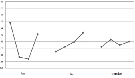
RPDs. Also means of RPD and S/N ratio are depicted in Fig. 2 and Fig. 3. According to these

Fig. 2. The average S/N ratio plot at each level for RPD for algorithm calibration

Fig. 3. Main effects plot for RPD values for algorithm calibration

Table 2

ANOVA input data for S/N ratios

Source DF Seq SS Adj SS Adj MS F P

Rm 3 2.74 2.74 0.9133 0.13 0.941

Rc 3 17.715 17.715 5.9049 0.82 0.528

Pop size 3 84.549 84.549 28.1829 3.92 0.073

Residual Error 6 43.129 43.129 7.1881

Total 15 148.132

Table 3

ANOVA RPD input data

Source DF Seq SS Adj SS Adj MS F P

Rm 3 0.06569 0.06569 0.0219 0.05 0.982

Rc 3 1.03122 1.03122 0.34374 0.83 0.522

Pop size 3 5.40573 5.40573 1.80191 4.37 0.059

4.2 Results

To evaluate the performance of the proposed model, eight different problems are considered shown in Table 4. Note that we consider the small-size problems since we compare the performance of GA algorithm and exact solution together. Since assembly details and scheduling aspects are not considered in the literature as the proposed models, the required data related are not available.

Therefore, these input data are generated randomly.For each test problem, the model has been solved

by LINGO 8.0 and compared with other two cases as follows:

1- For the first case, the model does not consider the scheduling. Therefore the objective function is to minimize the intercellular movements resulting due to processing and assembly operations.

2- For the second case, the model does not consider both the scheduling and the assembly details.

Table 4

The information of the eight benchmark problems

Problem # Ref.

Problem specification

Number of non-assembly Items

Number of assembly items

Number of Operations

Number of Machines

Number of Cells

1 McCormick et al.

(1972) 4 - 8 4 2

2 Xiaodan et al. (2007) 5 - 11 5 2

3 Heragu (1997) 6 - 15 7 2

4 Irani (1999) 6 - 14 10 3

5 Panchalavarapu and

Chankong (2005) 7 7 15 8 2

6 Singh et al (1996) 8 - 23 6 2

7 Chan & Milner

(1982) 10 - 46 15 3

8 McAuly (1972) 10 - 39 12 3

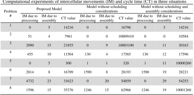
Table 5 summarizes the results of solutions and a comparison between the intercellular movements (IM) and cycle times (CT) for three situations. The computer machine used for solving is Pentium IV with CPU 2.GHz and RAM 1 GB.

Table 5

Computational experiments of intercellular movements (IM) and cycle time (CT) in three situations

Problem #

Proposed Model Model without scheduling

considerations

Model without scheduling and assembly considerations IM due to

processing

IM due to

assembly CT value

IM due to processing

IM due to

assembly CT value

IM due to processing

IM due to

assembly CT value 1

0 5 14216 0 0 16796 0 5 14216

2

51 4 7961 0 0 10009410 0 0 10584

3

2090 15 21855 0 9 10003100 0 11 30163

4

455 10 11504 130 4 17585 130 12 17596

5

0 5 300 1 1 320 1 11 10000260

6

2014 8 16709 1590 8 28193 1590 19 28221

7

4732 23 31623 0 20 54859 0 29 54253

8

In addition, using the proposed GA, the solutions are obtained and they are compared with corresponding solution of LINGO. The deviation of GA solution from the optimum value is calculated to compare the performance of the proposed GA with optimal solutions.

*

*

− =CTGA CT

Deviation

CT

Table 6

Computational results of the proposed method using direct implementation and GA

Problem # (i)

Optimum solution of LINGO Best solution of GA _{Deviation (D}

i) %

CT*value CPU Time CT value CPU Time

1 14216 00:00:01 14216 00:00:02 0.00%

2 7961 00:00:00 8017 00:00:03 0.70%

3 21855 00:00:01 23122 00:00:04 5.80%

4 11504 00:00:01 12896 00:00:03 12.10%

5 300 00:00:03 320 00:00:04 6.67%

6 16709 00:00:05 16709 00:00:04 0.00%

7 31623 00:01:58 32362 00:00:07 2.34%

8 35376 00:00:18 37054 00:00:07 4.74%

Based on results of Table 5, we can see that the CT* values of the integrated model are lower than the

time the model do not consider the scheduling parameters. Also, it is clear that the number of intercellular movements (IM) resulting due to assembly for model without assembly consideration is higher than the time this aspect is integrated with the CMS design problem. Table 6 also shows the details of the performance of the proposed model in terms of the CPU times and the objective function. As we can observe, there are two cases where both methods find the same optimal results and in other cases, the near-optimal solutions achieved by GA are fairly close to the optimal solutions.

5. Conclusion

In this paper, we have presented a new mathematical model for CMS design problem included cell formation and scheduling simultaneously where also the assembly operations and product structure are taken into consideration. The proposed model was formulated as nonlinear mixed integer programming and then has been simplified using some auxiliary binary variables. The resulted model was solved for some small problems and a GA method has been introduced to solve the proposed model for large-scale problems. The results of the proposed GA were compared with optimal solutions for some different problems in the literature. As a possible future research, one could consider the model with two objective functions including minimizing intercellular movements and minimizing cycle time of finished product.

References

Aryanezhad M. B. & Aliabadi J. (2010). Considering assembly operations and product structure for manufacturing cell formation. In proceeding of International Conference of Manufacturing Systems Engineering, Penang, Malaysia.

Boulif M. & Atif K. (2006). A new branch-&-bound-enhanced genetic algorithm for the

Chan, H. & Milner, D. (1982). Direct Clustering Algorithm for Group Formation in Cellular

Manufacture, Journal of Manufacturing Systems, 1(1), 64-76.

Franca, P. M., Gupta, J. N. D., Mendes, A.S., Moscato, P., & Veltink, K.J. (2005). Evolutionary algorithms for scheduling a flowshop manufacturing cell with sequence dependent family setups, Computers & Industrial Engineering 48, 491–506.

Ghosh, T., Sengupt, S., Chattopadhyay, M. & Dan, P. K. (2010). Meta-heuristics in cellular

manufacturing: A state-of-the-art review. International Journal of Industrial Engineering

Computations, 2(1), 87-122.

Heragu, S. S. (1997). Facilities Design, Boston: PWS Publishing Company.

Holland, J. (1975). Adaptation in natural and artificial systems. Ann Arbor: University of Michigan Press.

Hu, L. & Yasuda, K. (2006). Minimizing material handling cost in cell formation with alternative

processing routes by grouping genetic algorithm, International Journal of Production Research,

44(11), 2133–2167.

Irani S., (1999). Handbook of Cellular Manufacturing Systems, New York, NY: John Wiley & Sons,

Inc.

Johnson, D. J., (2005). Converting assembly lines to assembly cells at Sheet Metal Products: insights

on performance improvements, International Journal of Production Research, 43(7), 1483–1509.

McAuley J. (1972), Machine grouping for efficient production, The Production Engineer, 51, 53–57.

McCormick, W.T., Schweitzer, P.J., & White, T.W. (1972). Problem decomposition data

reorganization by a clustering technique. Operation Research, 20(5), 993–1009.

Onwubolu G.C. & Mutingi M. (2001). A genetic algorithm approach to cellular manufacturing

systems, Computers & Industrial Engineering 39: 125-144.

Park, M.W. & Kim, Y. D. (2000). A branch and bound algorithm for a production scheduling

problem in an assembly system under due date constraints. European Journal of Operational

Research, 123, 504-518.

Panchalavarapu P. R. & Chankong V. (2005). Design of cellular manufacturing systems with

assembly considerations, Computers & Industrial Engineering, 48, 449–469.

Reeves, C. (1995). A genetic algorithm for flow shop sequencing, Computers and Operations

Research, 22 (1), 5-13.

Ruiz R., Morato C. & Alcazar J. (2006). Two newrobust genetic algorithms for the flowshop

scheduling problem, Omega, 34, 461–476.

Schaller, J.E., Gupta, J. N. D., & Vakharia, A.J. (2000). Scheduling a flowline manufacturing cell

with sequence dependent family setup times, European Journal of Operational Research, 125,

324-339.

Sengupta, K. & Jacobs, F. R. (2004). Impact of work teams: a comparison study of assembly cells

and assembly line for a variety of operating environments, International Journal of Production

Research, 42(19), 4173–4193.

Singh, N. & Rajamaani, D. (1996). Cellular Manufacturing Systems: Design, Planning and Control,

Chapman and Hall, New York.

Tavakkoli-Moghaddam, R., Gholipour-Kanani, Y., & Cheraghalizadeh R., (2008). A genetic algorithm and memetic algorithm to sequencing and scheduling of cellular manufacturing

systems, International Journal of Management Science and Engineering Management 3(2),

119-130.

Wu J. & Hamada M., (2002). Experiments: Planning, Analysis, and Parameter Design Optimization.

Wiley.

Wu X., Chu C. H., Wang Y., & Yue D. (2007). Genetic algorithms for integrating cell formation with