www.biogeosciences.net/10/4957/2013/ doi:10.5194/bg-10-4957-2013
© Author(s) 2013. CC Attribution 3.0 License.
Biogeosciences
Geoscientiic
Geoscientiic
Geoscientiic
Geoscientiic
Automated quality control methods for sensor data: a novel
observatory approach
J. R. Taylor1,2and H. L. Loescher1,2
1National Ecological Observatory Network, Boulder, Colorado, USA
2Institute for Arctic and Alpine Research, University of Colorado, Boulder, Colorado, USA
Correspondence to:J. R. Taylor ([email protected])
Received: 5 November 2012 – Published in Biogeosciences Discuss.: 14 December 2012 Revised: 14 June 2013 – Accepted: 16 June 2013 – Published: 24 July 2013
Abstract.National and international networks and observa-tories of terrestrial-based sensors are emerging rapidly. As such, there is demand for a standardized approach to data quality control, as well as interoperability of data among sensor networks. The National Ecological Observatory Net-work (NEON) has begun constructing their first terrestrial observing sites, with 60 locations expected to be distributed across the US by 2017. This will result in over 14 000 auto-mated sensors recording more than>100 Tb of data per year. These data are then used to create other datasets and sub-sequent “higher-level” data products. In anticipation of this challenge, an overall data quality assurance plan has been developed and the first suite of data quality control mea-sures defined. This data-driven approach focuses on auto-mated methods for defining a suite of plausibility test pa-rameter thresholds. Specifically, these plausibility tests scru-tinize the data range and variance of each measurement type by employing a suite of binary checks. The statistical basis for each of these tests is developed, and the methods for cal-culating test parameter thresholds are explored here. While these tests have been used elsewhere, we apply them in a novel approach by calculating their relevant test parameter thresholds. Finally, implementing automated quality control is demonstrated with preliminary data from a NEON proto-type site.
1 Introduction
Observational ecology has historically focused on plot-stand–ecosystem–watershed scales that are meant to be rep-resentative of a larger ecosystem or region. By
accepted, statistically defensible approaches when compar-ing whole measurement systems or individual instruments as part of a larger rigorous quality assurance and data qual-ity control program (Loescher et al., 2005; Ocheltree and Loescher, 2007).
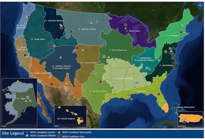
The NEON is currently constructing a continental-scale observatory consisting of 20 eco-domains in the US, in-cluding Alaska, Hawaii, and Puerto Rico (Fig. 1). Each of NEON’s eco-domains has one representative “core site” that will monitor the location continuously for 30 yr and two “re-locatable sites” that will also operate continuously but will move every 5–10 yr in order to address specific research di-rectives of interest for that domain (as decided by the re-search/user community). All the sites will contain a large suite of automated terrestrial sensors mounted on towers, placed in streams, and distributed in arrays of soil plots. In addition, 10 mobile towers (with supporting infrastructure) will be made available to rapidly deploy to targets of oppor-tunity that otherwise would not be able to capture key eco-logical information, e.g., immediately after a fire, flood, or insect outbreak. NEON’s construction is currently scheduled to end in 2017, at which time there will be more than 14 000 automated terrestrial sensors integrated into operations.
NEON is novel by design. It is the first ecological ob-servatory linking site-based organismal ecology with abiotic drivers and with regional spatial scaling. Taken in concert, these observations embrace the cause-and-effect paradigm. It is also novel in that each of these subsystems has been de-signed with the other subsystems in mind, making it the first truly integrated ecological observatory. By providing mea-surements/procedures that are traceable to nationally and in-ternationally recognized standards, a consistent, integrated, and interoperable approach can be used to enable a consis-tent means of data management and data quality. A com-plete description can be found in the NEON Science Strategy document (Schimel et al., 2011). NEON’s approach is at the forefront of many other observatories that are currently in-corporating interoperability into their design so as to enable a global “network of networks” (GEO, 2010; NRC, 2011; Suresh, 2012; IOM, 2013; USGCRP, 2013).
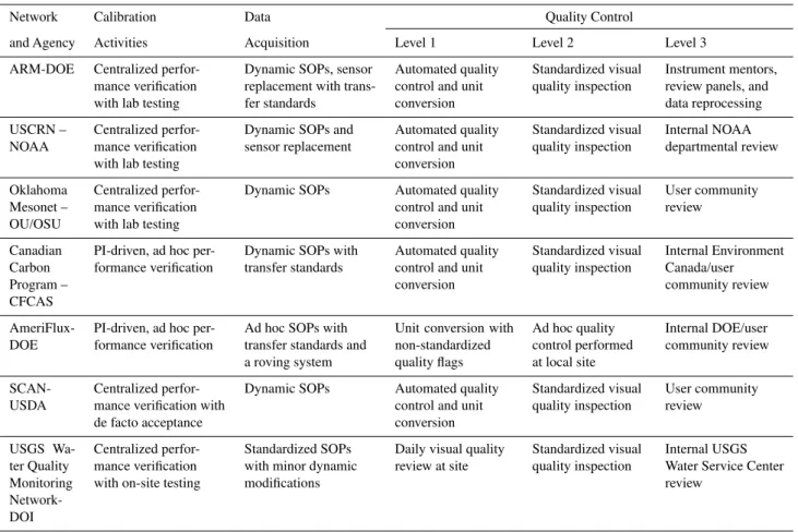
As large volumes of raw sensor data (>100 TB yr−1) are anticipated by these extensive, emergent networked obser-vatories, it is imperative that a comprehensive data quality assurance and quality control philosophy be adopted. In the broadest sense, quality assurance (QA) defines the overarch-ing plan for minimizoverarch-ing error and maximizoverarch-ing quality, while quality control (QC) refers to the actual procedures that are implemented as part of the QA plan (ISO/IEC 17025 2005, Peppler et al., 2008). While there is no universal QA/QC sys-tem for optimizing data quality, a number of common ap-proaches have been implemented by large observation-based networks (Table 1). In an effort to devise an efficient and effective quality assurance program for NEON’s automated terrestrial measurements, the optimal components of these
various quality assurance programs have been adopted (Tay-lor and Loescher, 2011).
A core premise in the formalism of complex quality con-trol is to scrutinize the validity of data in a multitude of ways and to consider as many different types of error as possi-ble (Gandin, 1969). To achieve this, NEON’s QA plan was based on a traditional “three-stage” approach to data quality control (Durre, 2008). The first stage focuses exclusively on automated quality control procedures in which all acquired data are screened by automated algorithms to identify sus-pect data that are then flagged for further investigation in the next stage. This second stage of QC performs data verifica-tion by means of visual inspecverifica-tion; any flagged data from the previous stage is either verified as being of poor qual-ity or is accepted as high-qualqual-ity data that are evidentiary of an uncommon event. This approach minimizes the risk of inadvertently eliminating the observation of a rare and po-tentially interesting event for the sake of data quality (Es-senwanger, 1969), and is consistent with the main principle of complex QC in that no decision about the data is made until all possible forms of QC tests have been performed (Gandin 1988). The third stage relies on independent audit-ing of the accepted dataset through an internally consistent (NEON) auditing plan as well as through external input from the user community. The end result is data that are of the highest quality and are maintained at this level through nec-essary reprocessing of data and version control. It should also be noted that a robust QA/QC plan also includes steady-state sensor calibration to traceable standards, and field validation activity, which are not the subject of this study.
This paper will focus exclusively on the automated QC methods that occur in the first stage, which are commonly referred to as plausibility tests (O’Brien and Keefer, 1985; Foken and Wichura, 1996; Foken et al., 2004; Fiebrich et al., 2010). Other aspects of automated quality control, such as redundancy tests, time series analysis, comprehensive uncer-tainty estimation, etc., will be addressed in a later paper. Be-cause of NEON’s large network size and 30 yr observational lifetime, it is prudent to adopt a “data-driven approach” for the first stage of automated QC. The principal philosophy behind this approach is to optimize human resources (both in the field and in the lab) by maximizing computer automation (Smith et al., 1996). While the implementation of fully auto-mated approaches has been well documented for individual observation sites (Meek and Hatfield, 1994), it has proven to be challenging for large networks (Shafer et al., 2000).
Fig. 1.NEON’s 20 eco-domains and their associated ecological research sites. “Core sites” monitor the ecosystem continuously for 30 yr while “relocatable sites” are moved every 5–10 yr in order to address specific research questions in a given domain. Some aquatic sites also include an embedded experiment called STREON (see the NEON Science Strategy document for more details; Schimel et al., 2011).
automated quality control methods, decisions are often based on arbitrary rules and can be implemented in inconsistent, ad hoc ways. The robust, automated QA/QC methods proposed here are further motivated by the need to optimize staff effort for field maintenance, which has direct budgetary implica-tions for long-term observaimplica-tions.
In practice, plausibility tests are essentially binary “pass/fail” checks that are automatically applied to every sin-gle observation (Graybeal et al., 2004). The pass/fail param-eters for each test are calculated directly from the data and stored in look-up tables. Because these parameters will be unique for each sensor, each measurement type, and each lo-cation, they will need to be dynamically updated on a reg-ular basis and, potentially, be maintained at a seasonal or monthly resolution. The theoretical basis for establishing this approach, as well as a novel methodology for implementing it, is the objective of this paper. A simple example applied to a limited number of sensors will also be shown. Finally, the limitations of this QC approach will be discussed.
2 Theory
2.1 Plausibility tests
Plausibility tests can broadly be defined as metrics that ex-amine the range and variability of a given dataset. Here, we describe these tests and how they are applied to the data. It should be noted that nature of sensor data often depends upon the phenomenon measured and not all of these tests will be applicable to every situation. Where possible, examples are used to demonstrate the efficacy of a given test. We apply this approach to observational data collected from a sensor, and assume (i) its field deployment is designed to best capture the phenomena of interest and minimize other systematic biases (Munger et al., 2012), and (ii) more advanced data products derived from multiple sensor datasets may require additional QA/QC approaches.
Table 1.Example quality assurance plans currently in use at large environmental observatories.
Network Calibration Data Quality Control
and Agency Activities Acquisition Level 1 Level 2 Level 3
ARM-DOE Centralized perfor-mance verification with lab testing
Dynamic SOPs, sensor replacement with trans-fer standards
Automated quality control and unit conversion
Standardized visual quality inspection
Instrument mentors, review panels, and data reprocessing
USCRN – NOAA
Centralized perfor-mance verification with lab testing
Dynamic SOPs and sensor replacement
Automated quality control and unit conversion Standardized visual quality inspection Internal NOAA departmental review Oklahoma Mesonet – OU/OSU Centralized perfor-mance verification with lab testing
Dynamic SOPs Automated quality control and unit conversion Standardized visual quality inspection User community review Canadian Carbon Program – CFCAS
PI-driven, ad hoc per-formance verification
Dynamic SOPs with transfer standards
Automated quality control and unit conversion Standardized visual quality inspection Internal Environment Canada/user community review AmeriFlux-DOE
PI-driven, ad hoc per-formance verification
Ad hoc SOPs with transfer standards and a roving system
Unit conversion with non-standardized quality flags
Ad hoc quality control performed at local site
Internal DOE/user community review
SCAN-USDA
Centralized perfor-mance verification with de facto acceptance
Dynamic SOPs Automated quality control and unit conversion Standardized visual quality inspection User community review USGS Wa-ter Quality Monitoring Network-DOI Centralized perfor-mance verification with on-site testing
Standardized SOPs with minor dynamic modifications
Daily visual quality review at site
Standardized visual quality inspection
Internal USGS Water Service Center review
Note: The Atmospheric Radiation Monitoring Network (ARM) is supported by the United States Department of Energy (DOE), (Stokes and Schwartz, 1994)
http://www.arm.gov/; the United States Climate Research Network (USCRN) is supported by the National Oceanic and Atmospheric Administration (NOAA), (Karl et al., 1995) http://www.ncdc.noaa.gov/crn/; Oklahoma Mesonet is supported by the University of Oklahoma (OU) and Oklahoma State University (OSU) (McPherson et al., 2007) http://www.mesonet.org/; the Canadian Carbon Program is supported by the Canadian Foundation for Climate and Atmospheric Science (CFCAS) (Margolis et al., 2006) http://www.fluxnet-canada.ca/; the AmeriFlux Network is supported by the United States Department of Energy (DOE) (Baldocchi et al., 2001)
http://public.ornl.gov/ameriflux/; the Soil Climate Analysis Network (SCAN) is supported by the United States Department of Agriculture (USDA) (Schaefer et al., 2007) http://www.ars.usda.gov/main/main.htm; and the United States Geological Survey (USGS) water quality monitoring network is supported by the United States Department of the Interior (DOI) (Wagner et al., 2006) http://water.usgs.gov/owq/.
Two separate and distinct tests are used to check for a re-alistic fluctuation of values over a designated period of time: the “sigma test” and the “delta test”. The sigma test uses the standard deviation or variance of the data over a given period of time and compares it to a given threshold value (thresh-old definition is discussed below). If the standard deviation is below this sigma threshold then the observations have not varied realistically and the test is failed. The delta test exam-ines the difference between pairs of subsequent observations over a given time period. If the difference is less than the specified delta threshold, then the observations have not var-ied realistically and the test is failed. By using both of these tests in tandem, an instrument may appear to be function-ing correctly but its output that is “stuck” at a constant or near-constant value can be identified. For example, a radia-tion sensor that is completely covered with snow may report that there is adequate fluctuation between subsequent mea-surements (i.e., pass the delta test), but the variance over a
24 h period will be lower than expected because it is not able to view the daily change in solar radiation (i.e., fail the sigma test). Therefore, these tests would flag the data over this 24 h period as implausible.
result in realistic data variation (i.e., pass the step test) but have an increased number of dropped data points (i.e., fail the null test), so these data would be flagged as implausible. Identifying both the duration and the frequency of gaps in a given time series is crucial for later stages of quality control, such as gap-filling and error analyses, and has significance in the interpretation of natural variations, such as diurnal cycles, seasonal cycles, etc.
2.2 Test thresholds
The automated application of these binary plausibility tests is rather straightforward. It is, however, the estimation of the parameter “thresholds” of these tests that poses the greatest and most critical challenge. The statistical assumptions dic-tate that these threshold parameters are ideally defined by having a distribution of values that are objectively consid-ered “reasonable” for every sensor at every site. The range, step, delta, sigma, null, and gap parameter thresholds can all be rigorously determined by constructing statistical distribu-tions based on existing data over a period sufficiently long to capture the full suite of variability. A representative dis-tribution of range values, for example, is more effective than simply using historical minima and maxima as there is no way to ensure that these data themselves are reasonable, are of quality, and are relevant in a changing climate.
Because the sensors monitor physical quantities that span numerous distributions, it is not always possible to assume one fundamental statistical distribution and calculate the de-sired threshold quantities. However, as the point of interest is not with the distribution of the data but rather with a sta-tistical quantity derived from these data, a sampling distribu-tion of the statistic can be constructed. Since sampling dis-tributions are constructed from independent randomly sam-pled data, the central limit theorem states that the distribution will approach a Gaussian distribution as the number of sam-ples approaches infinity (Rice, 2007). Therefore, regardless of the nature of the underlying data, a properly constructed sampling distribution of a statistic based on these data will always follow a Gaussian distribution:
f (x)=√ 1
2π σ2 e−
(x−µ)2
2σ2 , (1)
wherex is any random variable, µ is the population mean of the random variable, and σ is the population standard deviation of the random variable. For example, a statistic for the minimum temperature at a given location will have a Gaussian distribution constructed from minimum temper-ature data points (discrete samples) over desired tempo-ral periods (e.g., hourly, diurnal, monthly, seasonal, annual, decadal, etc.). From this sampling distribution, inferences about the population mean minimum temperature and popu-lation minimum temperature standard deviation can be used to define the minimum temperature value that will be used as the threshold parameter for plausibility testing.
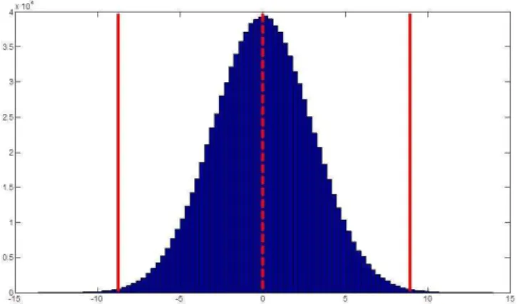
Because the Gaussian distribution is unimodal and sym-metric, the random variable can be normalized by the stan-dard deviation to yield a curve with the mean value centered at zero (see Fig. 2). When this analysis is completed, the in-tegral betweenµ−3σ andµ+3σ represents 99.7 % of all the data, and the integral overµ−2σ andµ+2σ represents 95 % of all the data. By exploiting these properties, we can define consistent and objective threshold parameters for all plausibility tests and, as the data volume increases, these val-ues can easily be reassessed and updated.
Although these parameters can be constructed for all tests, the exact details of the test, such as the sampling period and sample size, will vary depending on the type of observation and sensor. Because these emergent observatories, such as NEON, will be measuring new physical quantities, it may be challenging at times to find enough prior existing data to adequately construct sampling distributions. In these cases, best possible estimates of appropriate test parameters will be constructed for initial plausibility tests and, after a sufficient amount of NEON data have been collected, new parame-ters will be estimated and periodically updated. In this sense, this data-driven approach requires a “spin-up time” for suffi-cient data to be available for informing threshold parameter calculations. As observatories continue to make long-term observations, these threshold parameters will require regu-lar maintenance as they will be frequently recalculated from augmented data records.
As is inevitable with almost all statistical inference, there is an element of arbitrary choice in the decision level at which the test parameters are defined. Because plausibility tests are typically the first stage of quality control, it is prudent to esti-mate these parameter thresholds such that these tests should err on the side of heightened sensitivity. This is based on the philosophy that it is better to flag good data and verify that it is acceptable in the second stage of quality control rather than neglect to flag poor quality data and have it be published as plausible.
Fig. 2.Histogram of simulated data following a Gaussian distribu-tion with normalized mean 0 (dotted red line) and standard deviadistribu-tion of 3. The range of values that lie between 3 standard deviations of the mean (solid red lines) represent 99.7 % of all the data.
The sigma test relies on the variance/standard deviation of the sample in a predetermined sampling time (Table 2). It, in essence, scrutinizes the “standard deviation of the standard deviations”. Consequently, a sampling distribution of all the sampled standard deviations of the dataset will provide an in-ference of the minimum/maximum expected variability of a given parameter. A threshold ofµ±2σ (whereµrepresents the mean standard deviation of the distribution andσ is the standard deviation of the distribution of standard deviations) ensures that only the lowest/highest 2.5 % variability data is flagged. In many cases, care must be taken when scrutinizing the validity of this value and it will often need to be used in conjunction with other plausibility tests to assure data qual-ity. For example, if there is no precipitation over a three day period (a very realistic case), the sigma test alone would re-ject these data as having 0 variability. This false failure can be corrected by having two-stage tests where “0 variability conditions” are checked for consistency against other obser-vations and/or plausibility tests.
Similar to the sigma test the delta test scrutinizes the vari-ability of a dataset, but it focuses more on the observed small-scale random variability (i.e., noise) rather than the total sampled variability of a measured phenomenon over a specified period. The delta test utilizes the difference be-tween subsequent observations to check changes in the char-acteristic random variability. The mean and standard devia-tion of this sampling distribudevia-tion represent how small-scale random variability is correlated between subsequent obser-vations throughout the desired time series. If this quantity changes less than theµ−2σ threshold, data are flagged as being possibly “frozen” at a given value. Again, care must be taken with this test to ensure that observations that com-monly read 0.0 are not being inadvertently flagged when the zero values are real natural phenomena. In some cases, it may be advantageous to define the delta test threshold by the sampling precision of the instrument/data acquisition system,
rather than statistical analysis of the time series alone. For example, if the resolution of the instrument is 0.005, then it may be more appropriate for the delta test to utilize a thresh-old of∼0.01 to test if values are frozen and only vary near the instrument’s resolution.
The same distribution of subsequent observation differ-ences is used to also define the threshold for the step test (Ta-ble 2). Rather than scrutinize the smallest accepta(Ta-ble change between measurements, this step test seeks to ensure that there are no implausible, large increases in the variance struc-ture between/among measurements. The threshold is defined asµ+2σto ensure that only data exhibiting the largest 2.5 % of all data discontinuities are flagged. However, for this test to be applied to paired data points in an automated fashion, it is simplest to flag both points, thereby resulting in more flags than the 2.5 % would indicate. A subsequent process-ing of the flagged data (i.e., in the “data verification” stage of QC) could then help identify which of these flagged values is a distinct spike. However, if there is a sort of step-function change in the mean of the time series, then additional ver-ification will be required. It is for this reason that caution must be taken when applying this test and should be accom-panied by subsequent visual analyses of the time series for its validation. For example, wind speed and direction can typi-cally have large step changes that would be flagged by this approach when indeed the data are valid.
The null test and gap test are used to monitor the loss of data that could arise from problems associated with the in-strument, the data acquisition system, or both. The null test is intended to look for individual, missing data points within a given sampling period, while the gap test is meant to look for an extended period of missing data. The exact threshold for acceptable data loss will vary with the physical quan-tity being measured, the instrument, and sampling interval. In some cases, this may simply be defined as an arbitrary number (e.g., 0 or 1 maximum missing data value per day) or by a local calibration cycle. For data that are sampled as a continuous daily time series, the statistical approach that has been used to define all plausibility thresholds should con-tinue to be applied. A sampling distribution of the number of missing data values over a given sampling period should be constructed. In almost all cases, these two tests cannot be ap-plied to a raw time series without defining a sampling period in which a known number of samples is expected. As with other parameters, a threshold ofµ+2σis chosen for flagging data with the null test. It should be noted that these param-eters will only be representative of the sampling period, so any portion of the time series in which there are known gaps or null data points (e.g., during a calibration cycle) should be removed prior to estimating the sampling distribution. For data acquisition systems that do not report times with miss-ing data notation, a gap test must be used to explicitly check for missing data.
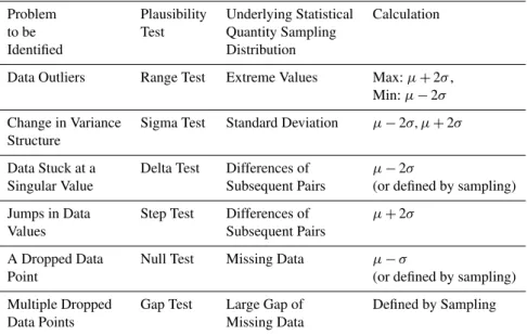
Table 2.The six plausibility tests employed in the first phase of NEON’s data quality control.
Problem Plausibility Underlying Statistical Calculation to be Test Quantity Sampling
Identified Distribution
Data Outliers Range Test Extreme Values Max:µ+2σ, Min:µ−2σ
Change in Variance Sigma Test Standard Deviation µ−2σ, µ+2σ
Structure
Data Stuck at a Delta Test Differences of µ−2σ
Singular Value Subsequent Pairs (or defined by sampling)
Jumps in Data Step Test Differences of µ+2σ
Values Subsequent Pairs
A Dropped Data Null Test Missing Data µ−σ
Point (or defined by sampling)
Multiple Dropped Gap Test Large Gap of Defined by Sampling Data Points Missing Data
While a Gaussian probability distribution function (Eq. 1) can be constructed manually from historical climate data for many variables, this process is computationally expensive and inefficient for the amount of data generated by large observatories. Without loss of generality, an algorithm that calculates the first two moments of a Gaussian distribution (the mean and variance, respectively) can be constructed dis-cretely to be
x (d)=
H (d)
P
y
x (d, y)
H (d)
P
y
1
(2)
σ2(d)=
H (d)
P
y
[x (d, y)−x (d)]2
H (d)
P
y
1
, (3)
wherex is a measurement statistic on a given day,d, with a historical dataset of measurements on this day,H (d), andx
andσ2are the derived mean and variance for this measure-ment statistic. For example, this could be a dataset of daily maximum temperatures observed at a specific location for 30 yr.
While this approach is computationally more efficient than manually constructing these parameters, it does not include all available information, such as temporally and spatially adjacent observations. Once an observatory’s (or network’s) operational phase has begun and there are more data repre-sentative of the spatial and temporal variation available, al-gorithms utilizing a combined approach for defining plausi-bility parameters will be more appropriate (Hasu and Aalto-nen 2011). As the spatio-temporal correlation length scales
are unique to each measurement statistic, a useful approach is to incorporate weighting factors for their respective influ-ence. This results in the following modifications to Eqs. (2) and (3):
xi(d)= Ni P j Dd P d′
H(d′)
P
y
w1(j, i)·w2 d′, d·xj d′, y
Ni P j Dd P d′
H (d′)
P
y
w1(j, i)·w2(d′, d)
, (4)
σi2(d)=
Ni P j Dd P d′
H(d′)
P
y
w1(j, i)·w2 d′, d·xj d′, y−xi(d) 2 Ni P j Dd P d′
H (d′)
P
y
w1(j, i)·w2(d′, d)
, (5)
whereNi is the set of neighboring sites measuring the same
quantity,Ddis the set of adjacent dates upon which the
quan-tity is measured, andw1andw2represent the spatial and
tem-poral weighting factors, respectively. These weighting fac-tors are defined as
w1(j, i)=
0, j /∈Ni
1, j =i
1 2e
−
|1ij| z
2
, j ∈Ni/{i}
w2 d′, d=
0, d′∈/Dd
e−
|d′−d| t
2
, d′∈Dd,
where |1ij| represents the distance between neighboring
are considered. The temporal weighting is based on observa-tions changing linearly with time, and the spatial weighting is based on traditional Barnes interpolation analysis (Barnes, 1964). When considering the values of these parameters, it is necessary to assess the coherent structure of the measure-ment variable and assign appropriate spatio-temporal scales. When all of the plausibility test parameters have been de-fined, the tests can be implemented in sequence for each observation at each site. In observatory operations, the en-tire testing procedure is automated in which individual data streams are checked prior to any other data manipulation (as part of the second phase of QC). It is important to note that this approach is only utilized for the definition of plausibility test parameter thresholds. Other internal tests, such as those for consistency and redundancy, should also be performed at a local site where spatio-temporal weighted observations may not be most appropriate.
3 Results and test examples
3.1 Defining parameter thresholds
3.1.1 Temperature data
The implementation of these automated plausibility tests is illustrated using temperature data from a NEON prototype relocatable site in North Sterling, Colorado (40.461903◦N, 103.029266◦W; Domain 10 – Central Plains in Fig. 1). These raw temperature observations were recorded in the form of voltage across a platinum resistance thermometer (PRT) (Barber 1950). It should be noted that these data were intentionally not calibrated and contain numerous known er-rors, which is useful for the purposes of this example.
A time series of 1 month of data sampled at 1 s intervals in April–May 2011 were chosen as the “historical dataset” for defining the threshold parameters for plausibility testing (Fig. 3). As there are no adjacent observations or histori-cal temperature records for this site, sampling distribution parameters described in Eqs. (4) and (5) simply collapse to Eqs. (2) and (3). The native sampling units of the PRT (mil-livolts) were used here for the sake of brevity. In practice, much more data will be used for defining threshold test pa-rameters.
From this time series, statistical sampling distributions were constructed by randomly sampling 100 data points, 1000 times. From each sample of 100 data points, a mean, standard deviation were calculated according to Eqs. (2) and (3), respectively. The statistical sampling distribution of these mean values is shown in Fig. 4. Note that with only 1000 samples, the shape of the distribution approaches that of the Gaussian shown in Fig. 2. By applying the central limit theorem to this distribution, the inferred population mean is 113.3 mV. In practice, the number of data points available
Fig. 3.Time series of platinum resistance thermometer (PRT) ob-servations in April–May 2011 from Domain 10: North Sterling, Colorado. These data were intentionally not calibrated and contain known errors.
will be constrained by the amount of available historical data and temporally/spatially coincident data.
Using the same sampling characteristics, a statistical sam-pling distribution of the upper and lower range limits (±2σ
for each extrema) can be constructed. From this distribution, the value of the upper threshold range can be inferred to be
µ+2σ =119.2+2×(0.74)=120.7 (see Fig. 5). It should be explicitly noted that daily extrema were not used in con-structing these sample distributions as this would not allow the data be independent and randomly sampled, as required in the construction of sampling distributions (although, in practice, a sufficiently large volume of data would remove this restriction). If a sufficiently large enough dataset of daily extrema were available (e.g., years of daily maximum tem-perature values), then this could be used as an alternative ap-proach for constructing these thresholds. With this threshold parameter now known, the range test simply consists of au-tomatically checking all of the data to ensure that any values above this threshold are flagged according to the above crite-ria.
In a similar fashion, all parameters for step testing, sigma testing, delta testing, and null testing were calculated by constructing sampling distributions (or, as previously men-tioned, they could be defined by the inherent data sam-pling/acquisition rate of the sensor).
3.1.2 Precipitation data
To illustrate the efficacy of this technique on data with an un-derlying non-Gaussian distribution, the same test parameter threshold definition procedure was carried out on precipita-tion data.
Fig. 4.Statistical sampling distribution of the sample mean PRT observation constructed from 1000 samples.
Fig. 5.Statistical sampling distribution of the sample mean maxi-mum PRT observation added to twice the sample standard devia-tion.
data have already gone through the rigorous QA/QC meth-ods employed by USCRN (https://www.ncdc.noaa.gov/crn/ qcdatasets.html), it is unlikely that any spurious data will be present to skew the test parameter threshold definitions.
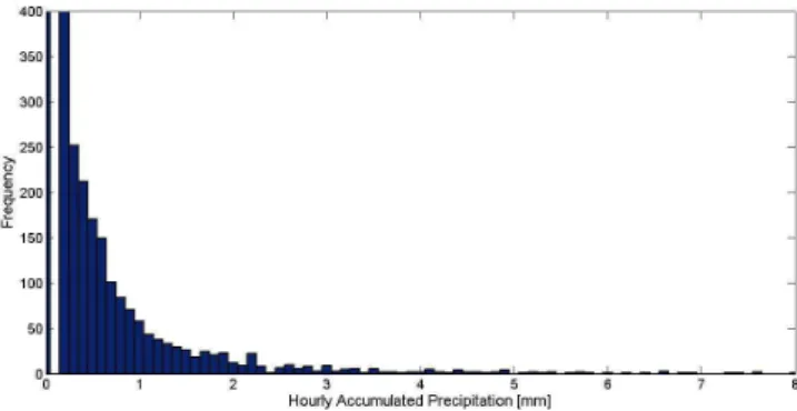
A time series of 2 yr of data sampled at 1 h intervals was chosen to demonstrate the naturally skewed distribution that is expected for midlatitude precipitation (Fig. 6). Due to the high volume of data, statistical sampling distributions were constructed by randomly sampling 10 000 data points 10 000 times, with replacement. It should be noted that these num-bers were chosen rather arbitrarily and, in practice, the size of the available dataset is often the limiting factor in choos-ing sample sizes. As with the temperature data, from each sample of 10 000 data points, a mean and standard deviation were calculated according to Eqs. (2) and (3), respectively. The statistical sampling distribution of the sample maxima is shown in Fig. 7. As is clearly evident, the statistical sam-pling distribution is closely approximating that of the Gaus-sian shown in Fig. 2, with an inferred population mean max-imum close to 1 mm h−1. This value is expected from the large number of nonrain events that occur at this site, which
Fig. 6.Distribution of hourly accumulated precipitation at the Boul-der, Colorado, USCRN site over 2009–2010. For visual purposes, the domain and range of this figure do not encompass all of the data. The true peak in the distribution actually has a frequency of over 15 000 for the zero precipitation event (0 mm accumulation), and there are some isolated events where more than 8 mm of pre-cipitation accumulates in an hour.
Fig. 7.Statistical sampling distribution of the sample mean max-imum hourly precipitation observation added to twice the sample standard deviation.
are assumed to be uniquely represented by the “zero val-ues” (that is, we are assuming that the sensor has always been in working order and that a reading of zero only repre-sents days without precipitation). The resulting range thresh-old parameters from this sampling distribution are [0, 1.12]. All values outside of this range should be flagged as poten-tially implausible. However, because the non-precipitation events (i.e., “zero values”) were included in the construction of the sampling distribution, the maximum threshold for rain events is biased toward a lower value than would typically be appropriate for automated plausibility testing. This exam-ple demonstrates the necessity of utilizing prior knowledge of the observational dataset to interpret the meaning of the thresholds that are derived.
Fig. 8.Time series of hourly accumulated precipitation observations in 2009–2010. The dotted redline is the range parameter threshold beyond which data should be flagged (∼2.3 % of the data should be flagged).
associated with theµ+2σ threshold defined in the preced-ing section. In practice, for a quantity such as precipita-tion, it would be advantageous to relax this definition to a value closer toµ+3σas variability associated with extreme events is common. It also should be noted that, in this ex-ample of high-quality data, these flagged values are entirely expected to be “revalidated” in the other phases of QA/QC (e.g., in comparisons with redundant sensors) and kept as high-quality data.
3.1.3 Other data
In the two previous examples, care was taken to choose the sampling windows and test parameters of interest to ensure that derived Gaussian sampling distribution was representa-tive of meaningful data quality control parameters. In some sense, the selection of these parameters is arbitrary, but there are definitely some parameters that are more optimized than others. When presented with the challenge of defining the parameters for automated plausibility testing on a number of different measurements, several factors should be consid-ered. In particular, the underlying temporal and spatial vari-ability of the quantity of interest must be considered. A broad based assumption is that a measurement is taken at a fre-quency (and spatial distribution) to capture the natural mean and variance structure of the desired phenomenon.
The primary factor was related to the underlying tempo-ral and spatial variability of the quantity of interest and how well measurement samples capture this variability. For exam-ple, ambient air temperature is a slowly changing quantity that typically follows a diurnal cycle. With a measurement sampling rate of 1 Hz, there is confidence that the natural variability of temperature will be well captured by the data. With such a large amount of data, statistical sampling distri-butions can be created that will adequately characterize the test parameter of interest (e.g., daily maximum temperature). Furthermore, when this is the case, “data windows” can be
defined in which subsets of data can be further scrutinized for plausible variability.
For the converse case, where a quantity of interest is a rapidly changing variable and it is not sampled very fre-quently, it is unlikely that the dataset will be representative of the true natural variability. For example, wind speed and direction is a quantity that changes rapidly, sometimes with diurnal dependence. If the wind were only measured once every hour, these observations would not be able to capture the actual variability of the wind, and any sigma or delta test parameters would not be applicable for plausibility testing, i.e., violating the assumption noted above. In such cases, it is recommended that plausibility test thresholds be set con-servatively so that data quality is heavily scrutinized a priori until such time that an adequate dataset can be compiled.
Irregularly occurring variables also pose some challenges. For example, precipitation measurements may have the ca-pability to observe with very high frequency, but as precip-itation does not typically follow a recurring cycle, its high degree of natural variability makes threshold definition very difficult. Most plausibility tests related to variability will of-ten not be applicable, nor will a minimum range value be useful (i.e., there are many days where no precipitation oc-curs). However, as illustrated in the example above, maxi-mum plausible hourly accumulated precipitation can be de-fined and utilized for automated quality control. This further demonstrates that the utility of a particular plausibility test is unique for each measurement.
Of course, if a novel measurement is being conducted for the first time and there is inadequate knowledge of the under-lying sampling distribution and its ability to capture natural phenomena, it will be challenging to determine any of these parameters. In such a case, it is recommended that plausibil-ity tests not be used at all until an adequate sample of these data is obtained for inspection first.
3.2 Application to test data
The same prototype temperature observations from Sect. 3.1.1 were used to illustrate the efficacy of plausibility testing by employing these calculated threshold parameters. A time series of 2 months of data sampled at 1 s intervals is shown in Fig. 6. This represents approximately 5.2×10⁶ data points. These data will be considered the “test” data upon which all of the plausibility tests should be conducted, and, via visual inspection, it is obvious that there are some poor quality data values (such as those that read “0 mV”). Using the derived test parameters, these data were processed with all six of the automated plausibility tests. The data that failed these tests were flagged (Fig. 7).
Fig. 9.Time series of platinum resistance thermometer (PRT) ob-servations in March–May 2011 from Domain 10: North Sterling, Colorado. These data were intentionally not calibrated and contain known errors.
– Range test: the range thresholds were found to be 104.04 to 118.56 mV. There were 150 643 values out-side of this range, resulting in 3.2 % being flagged. – Step test: the step threshold was found to be 0.2015 mV.
There were 36 values greater than this step resulting in 7.5 parts per million (ppm) being flagged, relative to the size of the total dataset.
– Sigma test: the sigma thresholds were found to be 2.57 to 3.56 mV. Because the observations in this dataset have considerable bias and variation (as intended), the lower sigma threshold was much larger than the antici-pated noise in the baseline observations. For this reason, the lower variance test was not applied and the plau-sibility of the variation over small timescales was as-sessed solely by the step tests and delta tests. While this is not nominally optimal, it does demonstrate appropri-ate use for datasets with large random variability (i.e., noise), such as this. Utilizing the test for only the upper sigma range and applied over a sliding window of 500 data points, there were 999 instances where the variance was greater than the acceptable sigma range, resulting in 0.02 % of the data being flagged.
– Delta test: due to the narrow range of variation in the observations, the delta threshold was found to be neg-ative and, consequently, set to 0 for this test. This will happen with observational datasets of this nature and should typically have a threshold set at the precise reso-lution of the sensor. For this particular prototype dataset, this value was not available and the delta test was not ap-plied. Nominally, the delta threshold would be applied over a rolling domain sequence of∼100 data points, or similar.
– Null test: the null threshold was found to be 12.6 miss-ing data points. This was applied over a movmiss-ing window
Fig. 10.Time series of platinum resistance thermometer (PRT) ob-servations in March–May 2011 from Domain 10: North Sterling, Colorado, but data that have failed QC tests are flagged as suspect. The different colored symbols represent the different flags that have been applied by the automated plausibility testing.
sequence of 50 data points resulting in 42 804 instances where there were more missing values than the thresh-old, causing 0.9 % to be flagged.
– Gap test: the gap threshold was chosen to be 5 min (this was an arbitrary choice and not based on any statisti-cal statisti-calculations). There were 116 time gaps greater than this threshold, resulting in 24 ppm being flagged. By combining all of the plausibility tests together, this re-sulted in 194 581 data points being flagged, or 4.1 % of all the data in question. It should be noted that many poor ob-servations were flagged by multiple tests, so the total number of flagged data points was not simply the linear addition of flagged data points from individual failed tests.
It should also be noted that these tests can be made more efficient through strategic sequencing. For example, data points that are flagged by the range test could potentially be disregarded when utilizing the sigma test. This would ensure that the sigma test is more representative of the true variance structure of the dataset in question and it will decrease the likelihood of data points getting flagged twice. Of course, there are circumstances where the nature of the observations does not lend itself to this sort of sequencing, so, as with all plausibility tests, the underlying structure of the data must be considered when making these decisions. The implemen-tation of such efficiencies at NEON is done through the use of a quality metric scheme that aggregates data quality flags to inform more sophisticated decision making. The details of this scheme will be discussed in a subsequent publication.
Fig. 11.Time series of platinum resistance thermometer (PRT) ob-servations in March–May 2011 from Domain 10: North Sterling, Colorado, but all of the flagged data have been removed, leav-ing only observations that passed all automated plausibility tests (∼4.1 % of the raw data was flagged).
phase-three QC. Consistent with NEON’s data-sharing pol-icy, records of the flagged data and complete quality control reports will be made freely available to all interested stake-holders. It is hoped that this policy of transparency and avail-ability will become the standard across all observatories and networks.
4 Discussion
4.1 Comparisons with other data quality control techniques
By using a data-driven approach to automated quality con-trol, human interaction is minimized and arbitrary decisions can be avoided. This objective approach avoids ambiguity that has traditionally been associated with quality control among different sensors and provides an extensive frame-work upon which observatories with long observational life-times can be sustained (e.g., NEON’s 30 yr planned lifespan). As part of an overall QA plan, this approach must be used in conjunction with other quality control and assurance proce-dures (phases 2–3).
In contrast to other QC approaches (such as those outlined in Table 1), this data-driven approach avoids the use of nu-merous assumptions. Many networks employ a subset of the plausibility tests discussed here in a way that utilizes static threshold parameters and/or relies heavily on human-based intervention. Utilizing these automated plausibility tests not only minimizes human action, it also allows for thresholds that are updated dynamically as more data are collected. In this sense, this QC approach “learns” from actual data and ultimately generates an optimized algorithm without any ex-plicit modeling of variable behavior. This avoids the need for assuming an underlying statistical distribution and eliminates all prognostic modeling. This is advantageous for many
vari-ables that have not been previously observed in a large-scale context and, therefore, are not well understood. Modeling the behavior of NEON’s 14 000 simultaneous observations is also computationally demanding, and potentially requires a significant level of verification and validation before it can be implemented in any automated way.
However, this approach is not without its limitations. In particular, the lifetime of an environmental observatory (e.g., NEON) and its focus on climate change could result in a record of observations where dynamic changes have sig-nificantly modified threshold parameters. For example, in a warming climate, temperature values that may seem excep-tionally high or variable in 2012 may in fact be well within normal conditions in 2042. As new data are collected and the threshold parameters are updated, it is inevitable that pub-lished data will need to be reprocessed into newer versions. Climatological averages are typically recalculated every 10 years, so it can be expected that these changes will occur at least this frequently.
The converse limitation is also true. As with most statis-tical approaches, there is inevitably an element of arbitrary choice when it comes to setting threshold limits. In the exam-ples shown here, a two-standard deviation offset was chosen for illustrative purposes. It should be noted that this resulted in a significant number of “false-positive” plausibility test re-sults in which seemingly good data were flagged (see Fig. 7). This problem is typically managed in a number of ways: (A) by choosing very liberal thresholds, (B) by implementing a second phase of quality assurance in which flagged values are further scrutinized, or (C) both. These options have their advantages and disadvantages. In choosing option (A), “good data” will very likely pass the tests and only the most egre-gious of implausible data points will be flagged. However, this approach does run the risk of allowing more “bad data” to be accepted as false negatives. In choosing option (B), more conservative thresholds can be chosen to ensure that as many of the implausible data points as possible are flagged. The downside to this approach is that all of the flagged val-ues need to be revisited in a second phase of data verification to sort the “good from the bad”, which consumes further re-sources. In the implementation of NEON’s QC approaches, option (B) has been chosen.
4.2 Toward better approaches
While automated data quality control through plausibility testing establishes the core of an efficient and sophisticated observatory quality assurance plan, it still requires long-term maintenance. To this end, it must be designed with sufficient flexibility to adapt to unforeseen quality control challenges that will undoubtedly arise in the future. To assist with en-hancing QC flexibility, we recommend complete records of data flags and quality control reports be maintained through-out the lifetime of the observatory. This permits the recalcu-lation of running statistics of how threshold parameters for particular measurements (and locations) behave over time, and will inform how to manage this challenge.
This record of data quality will be augmented by a thor-ough auditing plan that will not only scrutinize generated data but also the quality control of this data. Independent, random auditing is another method through which data QC can be tested for efficacy. This will consist of audits on real sensor measurements as well on test datasets that have ex-pected outcomes. Failure to meet audit goals will result in immediate scrutiny of the QC tests and be followed by sig-nificant testing and potentially reimplementation of the QC threshold parameters (and associated data reprocessing). All of these details will be included as part of the data quality record and should be part of the data providence and com-municated to the data-user community. While extensive data quality auditing requires additional resources, it is necessary to establish the “quality of quality control.”
One way to maintain flexibility within the quality control system is to ensure that all raw data are always archived. As data quality control evolves, having the raw data available ensures that reprocessing to enhance data quality can always be achieved. As part of NEON’s QA plan, the intention of QC is to identify (and remedy) problems, not simply eliminate data outliers. As such, no data should ever be deleted and the raw data should be permanently maintained by the host Observatory and freely available to interested data users. 4.3 Future applications
Automated, data-driven QC could easily be implemented at numerous other automated sensing networks. The most obvious candidate for this is meteorological observato-ries/networks. Often the historical construction of the infras-tructure utilized by most met services limits the capacity for such data-intensive QC. However, after an initial investment of resources to implement this system, the maintenance re-quired for this automated QC is minimal, and the resulting data quality enhancement would more than offset these costs. The question of how these automated QC tests would be ap-plied to historical data raises another set of issues that would need to be addressed on a case-by-case basis.
In addition to met services, there are many existing net-works (such as those in Table 1) that could benefit from more
automated QC techniques. Regardless of the measurement, instrumentation, and the cyberinfrastructure, these plausibil-ity tests can almost always be implemented and used to en-hance data quality. It is always necessary that this be imple-mented as part of an overarching QA plan and, depending on the observations of interest, may require very thorough data auditing. For instances where a series of data is processed using complex time series analysis (e.g., Fourier transforms, wavelet analysis, etc.), care must be taken to ensure that auto-mated corrections applied in one space do not yield spurious results in another space. For instance, the removal of out-liers from one time series could cause “jump discontinuities” that contribute to large oscillations or “ringing” in the Fourier transform of this time series. In these cases, data quality au-diting can be used to identify where risks of such results are probable, and the automated QC can be adjusted accordingly. For the vast majority of observations, these standard plausi-bility tests will be sufficient for enhancing data quality.
One of the biggest challenges for moving toward global datasets of observations is that of network interoperability. Without standardized approaches to network observations, no two sets of data can adequately be combined in any way. The future of network interoperability can only be en-hanced when a well-planned, uniform approach to data QC is adopted. While it is obvious that different observing net-works will have differing demands for QC approaches and implementation, “phase 1” plausibility tests will almost uni-formly be required in one capacity or another. Using these automated QC approaches can only assist with enhancing data quality and, consequently, data usage.
5 Conclusions
With the rapid growth of national and international sensor networks, the demand for data quality control in ecology will grow to an unprecedented level. Network interoperability can be best achieved by having unified approaches to QA/QC methods and, it is hoped, that the methods presented here will act as a primer for all other networks. By adopting methods that can be implemented rapidly, such as these, a consistent framework for data management can be established. It is only through the use of these standardized approaches that global-scale ecological questions can ever be addressed.
Foundation under the following grants: EF-1029808, EF-1138160, EF-1150319, and DBI-0752017. Any opinions, findings, and conclusions or recommendations expressed in this material are those of the authors and do not necessarily reflect the views of the National Science Foundation.
Edited by: P. Stoy
References
Baldocchi, D., Falge, E., and Gu, L.: FLUXNET: A new tool to study the temporal and spatial variability of ecosystem-scale car-bon dioxide, water vapor, and energy flux densities, B. Am. Me-teorol. Soc., 82, 2415–2434, 2001.
Barber, C. R.: Platinum resistance thermometers of small dimen-sions, J. Sci. Instrum., 27, 47–49, 1950.
Barnes, S. L.: A Technique for Maximizing Details in Numerical Weather Map Analysis, J. Appl. Meteorol., 3, 396–409, 1964. Brantley, S. L., White, T. S., White, A. F., Sparks, D., Richter, D.,
Pregitzer, K., Derry, L., Chorover, J., Chadwick, O., April, R., Anderson, S., and Amundson, R. : Frontiers in exploration of the critical zone: Report of a workshop sponsored by the National Science Foundation (NSF), 24–26 October 2005, Newark, USA, 2006.
DeFries R., Houghton, R. A., Hansen, M. C., Field, C. B., Skole, D., and Townshend, J.: Carbon emissions from tropical deforestation and regrowth based on satellite observations for the 1980s and 1990s, P. Natl. Acad. Sci. USA, 99, 14256–14261, 2002. Durre, I., Menne, M. J., and Vose, R. S.: Strategies for
Evaluat-ing Quality Assurance Procedures, J. Appl. Meteorol. Clim., 47, 1785–1791, 2008.
Essenwanger, O. M.: Analytical procedures for the quality control of meteorological data., Meteorological Observations and Instru-mentation: Meteorological Monograph, Am. Meteorol. Soc., 33, 141–147, 1969.
Fiebrich, C. A., Grimsley, D. L., McPherson, R. A., Kelser, K. A., and Essenberg, G. R.: The value of routine site visits in manag-ing and maintainmanag-ing quality data from the Oklahoma Mesonet, J. Atmos. Ocean. Tech., 23, 406–416, 2006.
Fiebrich, C. A., Morgan, C. R., McCombs, A. G., Hall Jr., P. K., McPherson, R. A.: Quality assurance procedures for mesoscale meteorological data, J. Atmos. Ocean. Tech., 27, 1565–1582, 2010.
Foken, T. and Wichura, B.: Tools for quality assessment of surface-based flux measurements, Agric. For. Meteorol., 78, 83–105, 1996.
Foken, T., Gockede, M., Mauder, M., Mahrt, L., Amiro, B., and Munger, J. W.: Post-field data quality control, in: Handbook of Micrometeorology, edited by: Lee, X., Massman, W., Law B., Kluwer Academic Publishers, Boston, USA, 181–203, 2004. Franklin, J. F., Bledsoe, C. S., and Callahan, J. T.: Contributions
of the Long-Term Ecological Research Program, Bioscience, 40, 509–523, 1990.
Gandin, L. S.: On automatic quality control of current meteorolog-ical information (in Russian), Meteorologiya i Gidrologiya, 3, 3–13, 1969.
Gandin, L. S.: Complex quality control of meteorological observa-tions, Mon. Weather Rev., 116, 1137–1156, 1988.
Graybeal, D. Y., DeGaetano, A. T., and Eggleston, K. L.: Improved Quality Assurance for Historical Hourly Temperature and Hu-midity: Development and Application to Environmental Analy-sis, J. Appl. Meteorol., 43, 1722–1735, 2004.
Group on Earth Observations (GEO): Report on Progress: Bei-jing Ministerial Summit, GEO Secretariat, Geneva, Switzerland, 2010.
Hanson, P. C.: New ecological insights through the Global Lake Ecological Observatory Network (GLEON), Ecol. Sci., 27, 300– 302, 2008.
Hasu, V. and Aaltonen, A.: Automatic minimum and maximum alarm thresholds for quality control, J. Atmos. Ocean. Tech., 28, 74–84, 2011.
Institute of Medicine (IOM): Environmental decisions in the face of uncertainty, The National Academies Press, Washington, DC, 209 pp., 2013.
ISO/IEC 17025: General requirements for the competence of testing and calibration laboratories, Second Edition, International Stan-dards Office, Geneva, Switzerland, 2005.
Karl, T. R., Derr, V. E., Easterling, D. R., Folland, C. K., Hofmann, D. J., Levitus, S.,Nicholls, N., Parker, D. E., and Withee, G. W.: Critical issues for long-term climate monitoring, Clim. Change, 31, 185–221, 1995.
Keller, M., Schimel, D., Hargrove, W., and Hoffman, F.: A conti-nental strategy for the National Ecological Observatory Network, Front. Ecol. Environ., 6, 282–284, 2008.
Loescher, H. W., Ocheltree, T., Tanner, B., Swiatek, E., Dano, B., Wong, J., Zimmerman, G., Campbell, J. L., Stock, C., Jacob-sen, L., Shiga, Y., Kollas, J., Liburdy, J., and Law, B. E.: Com-parison of temperature and wind statistics in contrasting envi-ronments among different sonic anemometer-thermometers, Agr. Forest Meteorol., 133, 119–139, 2005.
Margolis, H. A., Flanagan, L. B., and Amiro, B. D.: The Fluxnet-Canada Research Network: Influence of climate and disturbance on carbon cycling in forests and peatlands, Agr. Forest Meteorol., 140, 1–5, 2006.
McPherson, R. A., Fiebrich, C. A., Crawford, K. C., Elliott, R. L., Kilby, J. R., Grimsley, D. L., Martinez, J. E., Basara, J. B., Illston, B. G., Morris, D. A., Kloesel, K. A., Stadler, S. J., Melvin, A. D., Sutherland, A. J., and Shrivastava, H.: Statewide monitoring of the mesoscale environment: A technical update on the Oklahoma Mesonet, J. Atmos. Ocean. Tech., 24, 301–321, 2007.
Meek, D. W. and Hatfield, J. L.: Data quality checking for single station meteorological databases, Agr. Forest Meteorol, 69, 85– 109, 1994.
Munger, J. W., Loescher, H. W., and Luo, H.: Measurement, tower, and site design considerations, in: The Eddy Covariance Hand-book, edited by: Aubinet, M., Vesala, T., and Papale, D., Springer Verlag, 22–53, 2012.
National Research Council (NRC): A review of the U.S. Global Change Research Program’s Draft Strategic Plan. National Academies Press, Washington DC, 62 pp., 2011.
Ocheltree, T. O. and Loescher, H. W.: Design of the AmeriFlux portable eddy-covariance system and uncertainty analysis of car-bon measurements, J. Atmos. Ocean. Tech., 24, 1389–1409, 2007.
Peppler, R. A., Long C. N., Sisterson D. D., Turner, D. L., Bahrmann, C. P., Christensen, S. W., Doty, K. J., Eagan, R. C., Halter, T., Ivey, M. D., Keck, N. N., Kehoe, K. E., Liljegren, J. C., Macduff, M. C., Mather, J. H., McCord, R. A., Monroe, J. W., Moore, S. T., Nitschke, K. L., Orr, B. W., Perez, R. C., Perkins, B. D., Richardson, S. J., Sonntag, K. L., Voyles, J. W., and Wa-gener, R.: An Overview of ARM Program Climate Research Fa-cility Data Quality Assurance, Open Atmos. Sci. J., 2, 192–216, 2008.
Porter, J. H., Nagy, E., Kratz, T. K., Hanson, P., Collins, S. L., and Arzberger, P.: New Eyes on the World: Advanced Sensors for Ecology, Bioscience, 59, 385–397, 2009.
Rice, J. A.: Mathematical Statistics and Data Analysis, Third Edi-tion, Duxbury Press, Belmont, California, USA, 2007.
Schaefer, G. L., Cosh, M. H., Jackson, T. J.: The USDA Natural Resources Conservation Service Soil Climate Analysis Network (SCAN), J. Atmos. Ocean. Tech., 24, 2073–2077, 2007. Schimel, D., Keller, M., Berukoff, S., Kao, R., Loescher, H. W.,
Powell, H., Kampe, T., Moore, D., and Gram, W.: NEON Sci-ence Strategy: enabling continental-scale ecological forecasting, National Ecological Observatory Network, Boulder, Colorado, www.neoninc.org/science/sciencestrategy, 2011.
Schneider, D. C.: The rise of the concept of scale in ecology, Bio-science, 51, 545–553, 2001.
Shafer, M. A., Fiebrich, C. A., Arndt, D. S., Fredrickson, S. E., and Hughes, T. W.: Quality Assurance Procedures in the Oklahoma Mesonetwork, J. Atmos. Ocean. Tech., 17, 474–494, 2000.
Smith, S. R., Camp, J. P., Legler, D. M.: TOGA/COARE handbook of quality control procedures and methods for surface meteorol-ogy data, Tech. Rep. 96-3, Center for Ocean Atmospheric Pre-diction Studies, Florida State University, Tallahassee, FL, 1996. Stokes, G. M. and Schwartz, S. E.: The Atmospheric Radiation
Measurement (ARM) Program: Programmatic background and design of the Cloud and Radiation Test Bed, B. Am. Meteorol. Soc., 75, 1201–1221, 1994.
Suresh, S.: Research funding: Global challenges need global solu-tions, Nature, 490, 337–338, doi:10.1038/490337a, 2012. Taylor, J. R. and Loescher, H. W.: NEON’s Fundamental
Instru-ment Unit Dataflow and Quality Assurance Plan, NEON.011009, National Ecological Observatory Network, Boulder, Colorado, 2012.
United States Global Change Research Program (USGCRP): Cli-mate Assessment report; Third Assessment, 2013.
Wagner, R. J., Boulger Jr., R. W., Oblinger, C. J., and Smith, B. A.: Guidelines and Standard Procedures for Continuous Water-Quality Monitors: Station Operation, Record Computation, and Data Reporting, Tech. Rep. 1-D3, US Geological Survey, Reston, VA, 2006.