Dissertação apresentada à Universidade Federal de Viçosa, como parte das exigências do Programa de Pós-graduação em Genética e Melhoramento, para obtenção do título de Magister Scientiae.
LEANDRO GOMIDE NEVES
DETECTION AND MAPPING OF SINGLE FEATURE POLYMORPHISMS
(SFP) ON A HIGH-DENSITY SHORT OLIGONUCLEOTIDE ARRAY FOR
Eucalyptus spp.
VIÇOSA
Dissertação apresentada à Universidade Federal de Viçosa, como parte das exigências do Programa de Pós-graduação em Genética e Melhoramento, para obtenção do título de Magister Scientiae.
LEANDRO GOMIDE NEVES
DETECTION AND MAPPING OF SINGLE FEATURE POLYMORPHISMS
(SFP) ON A HIGH-DENSITY SHORT OLIGONUCLEOTIDE ARRAY FOR
Eucalyptus spp.
APROVADA: 05 de agosto de 2009
_____________________________ Dr. Dario Grattapaglia
(Co-Orientador)
_____________________________ Dr. Marcos Deon Vilela de Resende
(Co-Orientador)
_____________________________ Prof. Matias Kirst
_____________________________ Pesq. Danielle Assis de Faria
_____________________________ Prof. Acelino Couto Alfenas
Chamamos “explicação” o que nos distingue dos graus de conhecimento e de ciência mais antigos, mas isso não passa de “descrição”. Sabemos descrever melhor – explicamos igualmente pouco como nossos predecessores.
AGRADECIMENTOS
São muitas as pessoas que merecem menção por contribuírem para minha formação pessoal e profissional. Em especial, agradeço:
À Universidade Federal de Viçosa e ao programa de Pós-Graduação em Genética e Melhoramento, por apoiarem a realização deste trabalho.
À Coordenação de Aperfeiçoamento de Pessoal de Nível Superior (CAPES) pela concessão da bolsa de estudos durante o curso.
Ao professor Acelino Couto Alfenas, por me aconselhar e apoiar suportar minhas decisões.
Ao Dr. Dario Grattapaglia, a quem sou grato não só pelos ensinamentos técnicos, mas também, e principalmente, pela amizade e aconselhamentos.
Ao professor Matias Kirst, pela confiança em integrar-me ao seu grupo de pesquisa na Universidade da Flórida, permitindo que a maior parte do componente experimental fosse realizada.
Ao professor Giancarlo Pasquali e sua equipe, por receberem-me em seu laboratório na UFRGS durante a fase inicial do projeto.
Ao Dr. Marcos Deon, por ajudar-me em momentos importantes da análise dos dados do experimento.
À Márcia Brandão, por muitas ajudas, sempre com dedicação e paciência.
À Aracruz Celulose S.A. e ao Projeto Genolyptus por fornecerem e auxiliarem na coleta em campo do material biológico utilizado neste trabalho.
Ao Conselho Nacional de Desenvolvimento Científico e Tecnológico (CNPq) e à Empresa Brasileira de Pesquisa Agropecuária (Embrapa) pelo financiamento para a realização dos experimentos.
Àqueles que por muito tempo me acompanham com amizade incondicional, particularmente Thiago Reis, Vinícius, Leonardo, Tiago Soares, Luciano e Douglas.
A toda minha família pelo constante amparo - pais, irmãos, tios, primos e especialmente à minha avó Maria Cornélia.
Aos amigos do Laboratório de Genética Vegetal e da Embrapa, Juliana, Marco, Túlio, Rodrigo, Ediene, Leonardo, Samuel, Marília, César e Carol, por ajudarem em minha estadia em Brasília e amenizarem a rotina de trabalho.
Um agradecimento especial a Danielle Faria, por constantemente ajudar no desenvolvimento deste trabalho, mas principalmente pela amizade.
Aos amigos e colegas do mestrado, pelas horas compartilhadas estudando e descansando em Viçosa, particularmente ao Márcio e ao Ricardo.
A todos os amigos que me ajudaram enquanto estive na Flórida, entre eles Derek, Cynthia, Matthew, Evandro, Carol, Tania, Kathy, Gigi e Chris.
BIOGRAFIA
Leandro Gomide Neves, filho de Ary Rodrigues das Neves e Clara Maria de Brito Gomide, nasceu no dia 21 de janeiro de 1984 na cidade de Viçosa, Minas Gerais.
Obteve sua formação acadêmica inicial em Viçosa, concluindo o ensino médio no Colégio Universitário (COLUNI) em 2001 e graduando-se em Engenharia Florestal pela Universidade Federal de Viçosa em 2007. Seu interesse por Genética e Melhoramento iniciou-se após cursar um semestre de sua graduação na University of Minnesota Crookston e consolidou-se com a realização do trabalho de conclusão do curso sob a orientação do pesquisador Dario Grattapaglia na Embrapa – Cenargen.
CONTEÚDO
RESUMO... viii
ABSTRACT ...x
1. INTRODUCTION ... 1
2. LITERATURE REVIEW ... 6
2.1. Genetic maps for biology and breeding applications ... 6
1.2. Genetic maps on Eucalyptus... 8
1.3. Microarray technology ... 10
1.4. SFP technology ... 15
2. OBJECTIVES ... 18
3. MATERIAL AND METHODS ... 19
3.1. Eucalyptus pedigree selection ... 19
3.2. Microarray design ... 20
3.3. Tissue collection, DNA and RNA preparation and expression profiling ... 21
3.4. Microarray experimental design... 22
3.5. Selection of informative SFPs in the probe screening experiment ... 23
3.6. Full scale SFP genotyping and map construction... 24
4. RESULTS ... 26
4.1. Analysis of expression and microarray design... 26
4.2. Simultaneous detection and genotyping of SFPs in progeny data ... 28
4.3. Construction of a gene-rich map for Eucalyptus... 30
4.4. SFP identification using mixed-model analysis of variance ... 38
5. DISCUSSION ... 43
6. CONCLUSIONS ... 53
7. REFERENCES ... 54
RESUMO
NEVES, Leandro Gomide. M.Sc., Universidade Federal de Viçosa, agosto de 2009. Detecção e mapeamento de polimorfismo de sequência única
em uma população segregante de Eucalyptus spp. Orientador: Acelino
Couto Alfenas. Co-orientadores: Dario Grattapaglia e Marcos Deon Vilela de Resende.
ABSTRACT
NEVES, Lenadro Gomide. M.Sc., Universidade Federal de Viçosa, agosto de 2009. Detection and mapping of Single Feature Polymorphisms (SFP)
on a high-density short oligonucleotide array for Eucalyptus spp.
Adviser: Acelino Couto Alfenas. Co-Advisers: Dario Grattapaglia and Marcos Deon Vilela de Resende.
1. INTRODUCTION
Development of genetic maps has been a continuous and important step on the study of relevant biological phenomenon and on breeding applications. The types of markers used and the density of the genetic map are major characteristics that have been evolving over time. From phenotypic mutations that followed a Mendelian segregation [1] to the introduction of molecular markers, such as restriction fragment length polymorphisms (RFLPs) [2], greater marker density has been achieved. Among the class of molecular marker to be used, some explore random genomic regions while others explore pre-selected regions, a difference predominantly dependent on the degree of previous genomic information required by the technique. Although this might not seem limiting for model species, it is a crucial point for less studied organisms, which represent the majority of important commercial and ecological species and where genetic maps may be mostly useful.
This is the case of Eucalyptus, a genus comprising more than 700 tree and shrub species with original occurrence in Australia and adjacent islands, where some of these species have gained increasing silvicultural relevance to become one of the world most widely planted hardwood tree species. In spite of all its importance, breeding of selected genetic backgrounds is recent and the genera can yet be considered largely undomesticated, showing vast natural genetic diversity susceptible to be explored by forward genetics approaches concomitantly to classical breeding methodologies [3].
conformation polymorphism (SSCP), cleaved amplified polymorphic sequence (CAPS), denaturing gradient gel electrophoresis (DGGE), RFLP, microsatellite mining from expressed sequence tags (ESTs) and even SNP genotyping have limited throughput on organisms where genome is not fully sequenced or with high level of polymorphism resulted from outcrossing. As a consequence, few successful applications of these approaches are available for Eucalyptus, mostly allowing the mapping of a few dozen candidate genes.
For instance, Gion et al. [4] developed SSCP and CAPS markers and incorporated only eight lignin and symbiosis regulated genes to a reference RAPD map. As specific primers have to be designed for each gene, these methods are limited by the need to optimize polymerase chain reactions (PCR) and electrophoresis conditions to detect polymorphism and map the genes. Similarly, RFLP is a laborious process and design of probes on coding sequence to detect polymorphism also lacks throughput and, for example, only 31 cambium-specific ESTs and 14 known function genes were mapped by Thamarus et al. [5]. Comparable low-throughput results were also reported for pine species, another non-model outcrossing genera, even after considerable effort was employed on mapping genes [6].
On the other hand, DNA microarray technology has demonstrated to be a reliable platform for genomic studies. Since its development from complementary DNA microarrays [8], two key aspects allowed their application to less studied organisms, being (i) the ability to in situ synthesize oligonucleotide arrays [9] and (ii) the recent possibility to design custom arrays from some manufactures (as reviewed by [10]). Also, the principle that oligonucleotide arrays could be used to detect genetic differences between genotypes were first speculated [9] and then proved to be possible in the simple genome of yeast [11]. Nevertheless, only five years later it was demonstrated for the more complex genome of Arabidopsis by Borevitz et al. [12], who also termed this class of polymorphism as Single Feature Polymorphism (SFP).
The principle of SFP detection relies on the disruption of hybridization signal resulted from the hybridization of a sample that contains polymorphic loci between its genome and the reference sequence used to design the probes present on the array. If distinct genotypes are hybridized to the same array, sequence differences between them can therefore be ultimately detected as their hybridization patterns change [11].
Initially, genomic DNA was used as a hybridization source in yeast [11], Arabidopsis [12, 13], and rice [14], with the advantage that hybridizing equal amounts of genomic DNA for all samples suggests that every difference in signal is likely to be an SFP. However, due to a higher complexity, larger genomes tend to incorporate more noise when genomic DNA is hybridized to expression array.
based on differential expression of the gene, called gene expression markers (GEM), is also possible to be obtained [18].
Regardless of the source of polymorphism, generally called SFP unless otherwise stated, genotyping such markers in a segregating family and extracting those with Mendelian behavior ultimately should allow the development of high-density genetic map where the mapped markers represent genes for which the probe sets were originally designed. Consequently, SFP mapping can be summarized as a two-fold task involving the detection of probes that reveal putative SFP and their evaluation as Mendelian markers in a structured mapping population.
A major advance has been made to develop SFPs in model, self-pollinated, homozygous species. In these studies, identification of the putative SFPs has been made based on signal differences between the two original inbred lines. Subsequently, one would search and test for a bimodal distribution of these candidate markers in a sufficiently large mapping population typically made up of recombinant inbred lines or backcross progeny and genotype every individual using as a reference the signal intensity of the inbred parents [18-20].
hexaploid wheat were genotyped and had 877 SFPs allocated to a genetic map along with 269 microsatellites [22].
2. LITERATURE REVIEW
2.1. Genetic maps for biology and breeding applications
After the rediscovery of Mendel’s work on inheritance, it was realized by Punnet and Bateson that pairs of alleles might not independently segregate as proposed by Mendel, with those originally present in the parents happening more frequently in the progeny. The phenomenon was further studied by Thomas Hunt Morgan and this observation was attributed to the physical linkage of those loci on the same chromosome, guiding his group to postulate the principles of developing a genetic map. To explain differences in the proportion of alleles in the individuals of progenies from different crosses of Drosophila, Morgan speculated that crossing over of the chromosomes could be resulting in such recombination and that the more apart two genes are, the more likely crossing over is expected to occur. Following this assumption, Morgan’s student Alfred Sturtevant was the first to develop a genetic map [1].
The implications that genetic maps have had on biology and breeding since those pioneer works are enormous. The first markers used were phenotypic mutations that followed a Mendelian segregation and therefore were mapped in a large F2 population. Perhaps the first application resulting from genetic mapping, and indeed a very interesting one, was that Morgan predicted Drosophila to have 7,500 factors (genes) [1]. His educated guess was not only closer to the ~14,000 currently annotated genes [24] because the resolution of their map was not big enough due to a low density of markers.
genetic mapping to became more widely explored in biology and breeding, particularly after the development of restriction fragment length polymorphisms (RFLPs) [2]. Although these are very informative codominant markers, the development of polymerase chain reaction (PCR) let other classes of molecular markers to be generated, requiring less DNA and being less labor intensive. Random amplified polymorphic DNA (RAPD) were largely explored during the last decade and for many species, such as Eucalyptus, it was the first class of marker employed to create genetic maps, mostly because it does not require previous genomic information [23]. Shortly after, microsatellites became the marker of choice for genetic analysis resulting from its elevated polymorphic information content, transferability between different genetic backgrounds, capability of multiplexing several markers in a single reaction and easy detection on capillarity sequencers [25]. Early this decade single nucleotide polymorphisms (SNPs) have arisen as possible gold standard markers due to their large occurrence and evenly distribution on the genome, even though a single SNP is not a multiallelic marker [7].
As the generation of relatively dense maps became possible through the use of molecular markers, their applications on breeding started to be speculated. Genomic regions responsible for controlling a significant portion of the phenotypic variation, termed QTLs (quantitative trait locus) were identified and even major responsible genes were cloned underneath such QTLs [26, 27]. Practical applications of molecular markers, such as genotype identification and discrimination, germplasm characterizations and assessments of genetic diversity have also been reported in the literature (reviewed for forest species by [28]. Nevertheless, a more comprehensive application of such maps to marker assisted selection (MAS) is still lacking [3] and new approaches requiring an even greater marker density have been proposed, as is the case of genome-wide association (GWA) studies and genome-wide selection (GWS) [29, 30].
to detect sequence polymorphisms. This is the case of DArT (Diversity Arrays Technology) markers, a robust class of molecular marker that does not require previous genomic information but, as a consequence, interrogates anonymous regions for polymorphism [31]; and also of SFP (single feature polymorphisms) markers, which make use of some previous available genome information to design oligonucleotide DNA microarrays and interrogate these pre-selected regions for polymorphisms [12].
1.2. Genetic maps on Eucalyptus
The first genetic map was developed on Eucalyptus with RADP markers using a pseudo-testcross strategy [23]. RAPD markers were also used to fine map and detect a major gene responsible for rust resistance in a large full sib family of E. grandis [32], and preliminary studies involving QTL detection in Eucalyptus were also initially developed using this class of molecular markers [33, 34]. The use of RAPD markers make such results essentially not comparable across genetic backgrounds and consequently there was a shift towards the use of microsatellites for genetic and breeding analysis.
conditions have to be tested and optimized for each gene before ultimately detecting a mappable polymorphism. Therefore, those authors report the positioning of only eight genes on a RAPD map of Eucalyptus.
Thamarus et al. [5] made a more comprehensive effort to map genes on E. globulus pedigree essentially using the RFLP technology using probes for known genes. Probes were either already available for some of these genes from genomic and cDNA libraries developed by earlier studies, and some probes were derived for specific sequences by PCR amplification on genomic DNA. RFLP is a laborious methodology and those authors were able to map only 31 cambium-specific expressed sequence tags (ESTs) and 14 known function genes.
Another way of confidentially mapping genes is the in silico screening of EST libraries for microsatellite markers. This is a relatively efficient approach and markers keep the advantages intrinsic to microsatellites (et al. transferability, data quality, multiallelic). The method obviously requires microsatellites to be present in the ESTs and primers are developed flanking these regions, assuming that enough sequence is available for the EST to accommodate primers on both sides of the microsatellite. Regardless of these limitations, the amplification of the microsatellite can simply not work because the primers might have accidently been designed on an exon-intron border or because there is a sequence polymorphism between the primer sequence and the sample, which will preclude the hybridization of the primer to the predicted site. Furthermore, all the putative markers have to be screened for segregation and as a consequence high-throughput is not achieved, although one can map many genes depending on the EST library coverage and level of polymorphism of the pedigree [36].
map [37]. Similar to other low throughput technologies, the technique employed allowed mapping only a few genes. Other methods of SNP genotyping via high-density platform, such as the Illumina GoldeGate assay can also be used to genotype SNPs previously discovered in target genes [38], but its efficiency on highly polymorphic species of Eucalyptus with a nucleotide diversity above 1% has yet to be tested.
1.3. Microarray technology
With the development of genome sequencing projects of model species, such as yeast (Saccharomyces cerevisiae) and Arabidopsis thaliana, the physical structure of the genome became available for specific reference genotypes [39, 40]. Concomitantly, it was also realized that other functional information would be required for the understanding of the biology behind the sequences, particularly the role of the predicted genes in the organism. Although this is a very complex and yet unresolved question [41], understanding the transcription patterns of genes, for example the relative difference in expression between tissues or biological treatments, became possible with the advancement of DNA microarray technology [8].
Shortly, DNA microarray is an evolution of the classical southern blot procedure, where, instead of a few genes, it is possible to assign the expression level of every single gene of the organism. Another difference is that the DNA sequences representing the genes are now covalently bound to a small rectangle glass matrix. For example, Agilent’s microarray (Agilent technologies Inc.) measures around 7.5 cm by 3 cm, similarly to a microscope slide, and can fit up to one million features. On this surface, genes are allocated in a XY coordinate plane that allows the system to track back the signal to its relative gene [10].
Besides, sequencing a unique genotype obviously does not represent all polymorphisms present in the species, which is particularly relevant for species where interespecific hybridization is commonly used in breeding. This raises the question of where to extract the sequence information that will represent the genes and populate the microarray.
When DNA microarray technology was first developed, the pioneering work of Schena et al. [8], carried out even before the Arabidopsis’ genome was sequenced, used cDNA representing 64 genes spotted on glass by an automatic robot to represent the genes. In the forestry scenario, Kirst et al. [43] working with Eucalyptus also used spotted cDNA comprising 2,608 genes to populate the microarray, selecting them from a library of ESTs.
An interesting characteristic of cDNA microarrays resides in the fact that cDNAs are long fragments representing the transcribed part of the gene, being therefore robust to variation in signal due to length polymorphisms and SNPs between the sample and the library used to obtain the cDNAs. This means that if one is simply willing to measure gene expression levels in highly polymorphic species, the results would theoretically be less influenced by such class of polymorphism [44]. Nevertheless, spotted cDNA have the drawbacks of being labor intensive to produce, presenting several significant sources of variation that might confound the expression analysis and being more potentially affected by cross-hybridization problems [10].
particular gene. In other words, all the desired target genes would be represented by a probeset. One of the first versions of this format was a probeset of 20 probes, each one 25 bases long, constituting the Affymetrix GeneChip Array [9]. Wodicka et al. [9] were also the first to raise the possibility of using microarrays to detect genetic differences between genotypes.
A final significant evolution in the microarray technology came with the possibility to customize the probes that will be present on the array. This gives the researcher mobility to choose the regions of the genome one wants to consider most and the degree of coverage and redundancy allowed for each probeset (i.e. the number of probes per probeset). Longer probes can also be customized, up to 85-mer, although this size is constantly being improved. Such customization process allowed the construction of high-density in situ synthesized oligonucleotide arrays based on EST library information for species with unsequenced genome (reviewed by [10]).
Microarray analysis is prone to confounding sources of variance biasing the expression signal information. Appropriate experimental designs and statistical analyses have to be considered to account for these issues, allowing for the most accurate estimation of levels of gene expression. Even after controlling for these variations, inherent “noise” is a peculiar characteristic of microarray data, making confidence in the estimated parameters an important information extracted from appropriate statistical analysis. Kerr and Churchill [45] were some of the first authors to ask such questions and connect microarray experiments to classical experimental theory. For example, they illustrated the sources of variance commonly seen in a microarray experiment. They proposed the analysis of variance (ANOVA) as a way to separate biological variation from technical confounding effects and suggested new experimental designs based on classical experimental theory.
hybridized together to the array. Based solely on the relative red to green intensity signal a gene would be called differentially expressed (see picture 1 of [46].
It was quickly recognized that microarrays experiments could be designed in a factorial fashion and mixed-model analysis of variance could be used to test for significance in the main and interaction effects [46, 47]. Furthermore, the sources of variation in microarray data became largely understood and could be considered in a more appropriate experimental design, incorporating the principles of randomization, replication and blocking. For example, every microarray or slide is said to be an incomplete block with space for two treatments (the two dyes) and the genes or probes considered to be the fundamental experimental units [45, 48].
During the laboratorial part of a microarray experiment, several steps might introduce variation for specific genotypes that are neither biologically meaningful nor inherent to the microarray technique. Ideally, tissue collection, RNA extraction and every other subsequent reaction (labeling, hybridization, washing and scanning) should be performed in the same moment under the same exact conditions. However, when the experiment requires dealing and collecting samples from hundreds of genotypes this obviously becomes an unfeasible task and even more variation is incorporated. These examples of experimentally introduced variation that are not related to the biology, sometimes called “batch effects”, are a subset of variation that can be controlled by using appropriate experimental practices, as shown by Yang et al [49]. These authors presented comparable experimental data from four different laboratories to discuss that if batch and biological effects are confounded, it is impossible to extract reliable conclusions out of the data. As a result, reproducibility is compromised and comparisons between laboratories are inappropriate.
signal) and Cy5 (lower signal) dyes. Genotype (or treatment) effect indicates a case where particular genotypes have an overall signal difference from the remaining genotypes for the genes under study. At last, gene effect will show circumstances where certain genes show higher or lower signal compared to other genes [48]. Although it is believed that all these sources will contribute to variation in the data, the higher quality of the in situ synthesized oligonucleotide array tends to reduce their relative influence, for example reducing problems of gene effects, since equal amounts of DNA are synthesized on every microarray spot.
When measuring gene expression level, the second order interaction of genotype x gene is the effect of interest, indicating genes that have their signal intensities varying according to the genotype. Other combinations of second order interaction are due to technical variation and the higher third and fourth order interactions are assumed to be irrelevant [48]. Finally probe effects are present when a gene-level analysis is performed in oligonucleotide arrays, and significant genotype x probe interaction indicates genes with putative single feature polymorphism (see below).
To estimate components of variance for every effect as well as significance for effects of interest, a mixed-model analysis of variance is usually suggested, with slide effect and its interactions being considered random and the remaining effects considered fixed, except for the mean and the error, which are always assumed to be fixed and random, respectively [50, 51].
dyes. The loop starts when the first array is hybridized with the repetition two of the sample 1 and the repetition one of the sample 2; followed by the second array hybridized with the repetition two of the sample 2 and the repetition one of the sample 3; and the loop is continued until the last array, which is hybridized with the second repetition of the sample n and the repetition one of the sample 1 [52].
When compared to the reference design, the loop design is a robust experimental design for two-color microarrays that increases the number of observations for the samples of interest and has no confounding effects. It also provides degrees of freedom for estimating the error variance [48]. A final remark about the loop design is that it requires every sample to be labeled twice, which might increase the costs of the experiment without increasing the number of biological repetitions. Therefore, adaptations of this method to accommodate the experimental budget is possible if one assumes that the resulting confounding effects (if any) will not influence the analysis [53].
1.4. SFP technology
With the development of oligonucleotide arrays, the idea that sequence polymorphism would affect hybridization intensities, allowing for the detection of genetic differences between genotypes, was first speculated and later proved in yeast [9, 11]. The application of this principle to species with more complex genomes was only proved to be possible five years later by Borevitz el al. [12], to the yet relatively simple genome of Arabidopsis. Their work triggered a series of studies using DNA microarrays to detect polymorphism and this type of polymorphism was termed Single Feature Polymorphism (SFP).
differential expression between genotypes influence the hybridization signal and, therefore, complicates the detection of SFPs. For example, Wang et al. [20] demonstrated that the classical method developed by Winzeler et al.[11] is not the most efficient when expression is incorporated. Other advantages of using RNA rather than DNA are also reported on the literature, particularly the possibility to use the data for both expression analysis and genotyping and to obtain another class of polymorphism based on differential expression, called gene expression markers (GEM) [18].
While SFP is an inherent characteristic of a single probe of a probeset, a GEM is expected to change the expression profile of all the probes of that particular probeset. This can be explained by analyzing the genetic basis of each type of polymorphism. An SFP has its signal altered due to a SNP, insertion or deletion, or even a polymorphism generated during mRNA processing (e.g. alternative splicing and polyadenylation) [16]. On the other hand, the constitutive signal variation of the probes belonging to a probeset affected by a GEM is primarily a consequence of cis and trans-acting regulators of gene expression [19].
The position and number of polymorphisms present in the region explored by the probes play a major role on SFP detection. It has been reported that a greater chance of SFP detection occurs when the polymorphism is present on central regions when compared to the border of the probes [15, 17] and for cases where multiple polymorphisms exist [16]. The number of polymorphisms present along a probeset may also influence the SFP detection depending on the statistical method employed and most of the methods developed so far assume that there is one or only a few polymorphic probes per probeset [15, 54].
2. OBJECTIVES
The general objective of our work was to apply the SFP technology to large-scale mapping of genes in a reference map of Eucalyptus. This general objective can be broken down into four more specific objectives:
i) Design an in situ oligonucleotide microarray for Eucalyptus from previously available EST resources;
ii) Identify and genotype SFPs on a subset of a mapping population using the pseudo-testcross strategy;
iii) Develop a saturated gene-rich genetic map of Eucalyptus based on SFP genotyping;
3. MATERIAL AND METHODS
3.1. Eucalyptus pedigree selection
An interespecific cross between E. urophylla (U15) and E. grandis (G38) was selected for this study. The whole family comprising 250 individuals was planted in southern Brazil (State of Rio Grande do Sul) at Aracruz S.A. The experimental design used was in single tree plots with five blocks so that each individual was clonally replicated and five ramets were available for the study. A linkage map with 220 microsatellites markers was available for 188 individuals of this same family (Mamani et al. unpublished).
From the collected field grown trees, 28 biologically replicated individuals and 134 unique individuals were available for the subsequent analysis, all of them matching the microsatellite data set and with parentage and clonal confirmation after analysis of six highly informative microsatellites (Additional file 1).
between the two selected datasets and the remaining ones were taken in equal proportions from the non-overlapping to equally represent each parental map.
3.2. Microarray design
A Eucalyptus transcriptome custom array was ordered to perform the present study. Sequence information was available from the Genolyptus interespecific unigene set generated from ESTs derived from four species (E. grandis, E. urophylla, E. globulus, E. pellita) involving a total of 21,428 unique sequences [57].
The 21,428 unique sequences were submitted through Agilent’s eArray software tool to generate a total of 214,218 25-mer probes at a rate of 10 probes for every sequence. Shortly, the algorithm selects the 10 best sequences of 25 bases for each consensus according to an appropriate GC content, melting temperature and cross-hybridization probabilities to optimize hybridization conditions for the designed microarray. Also, a note with base composition (BC) and non-self perfect match (NSPM) scores is created as a quality index for every designed probe.
threshold, was designed to be used to hybridize the remaining progeny set previously sampled by selective mapping based on the microsatellite linkage data.
The microarray used for the full scale progeny genotyping included 43,777 probes selected from the results of the screening step. These probes represented 15,698 genes and were selected based on a set of criteria (see results). As a result, the full scale genoypying experiment used 17 Agilent customized arrays in a 4x44K slide format. The 26 negative control probes were again included on the array.
The sequence information for both screening and genotyping array is available upon request.
3.3. Tissue collection, DNA and RNA preparation and expression profiling
Differentiating xylem and expanded leaves was collected from each tree during a period of four consecutive days respectively for RNA and DNA extraction. An area of approximately 20 cm x 10 cm had the bark removed and the exposed tissue was collected by scraping this area (Additional file 3). The trees were 54 months old, growing under standard silvicultural conditions. Tissue collection was carried out in January 2008 during the active growing season to maximize transcript abundance. Immediately upon collection, tissues were stored in 50 mL sterile tubes under dry ice until they were lyophilized for further transportation and storage at room temperature. The parental trees were not planted on the area and could not be sampled. Nevertheless, frozen leaves were available for DNA extraction.
reaction followed the manufacturer recommendations. Electrophoresis was carried out on an ABI 3700 sequencer (Applied Biosystems, Foster City, CA, USA). Genotyping analyses were carried out using GeneScan 3.7 and Genotyper 3.7 (Applied Biosystems).
Total RNA extracted [59] from xylem tissue samples was treated with RQ1 RNase-free DNase (Promega, Madison, WI, USA), purified in mini spin columns (RNeasy Plant Mini Kit, Qiagen) and had the quality visually checked on agarose gels. Between 150 and 200 mg of lyophilized tissue was used for RNA extractions. Concentrations varied considerably according to tissue quality but absorbance ratios of 260/280 nm and 230/260 nm were generally between 1.8 and 2.2, as measured on a NanoDrop (NanoDrop products, Wilmington, DE, USA). The Two-Color Quick Amp Labeling Kit (Agilent Technologies, Santa Clara, CA, USA) was used to synthesize complementary RNA (cRNA) taking advantage of the low RNA input required. Manufacturer’s protocol was followed except for dividing all reagents’ volume by two to reduce costs. All samples yielded enough labeled cRNA for hybridization as recommended by the manufacturer. Samples were hybridized at the Interdisciplinary Center for Biotechnology Research (ICBR) of the University of Florida following Agilent’s protocol, except for lowering the hybridization temperature to 55 oC to compensate for the shorter probes. Randomization of all laboratorial steps was a rule whenever possible.
3.4. Microarray experimental design
3.5. Selection of informative SFPs in the probe screening experiment
Log2 transformed, quantile-normalized data for the 20,726 unigenes with expression profiled in 28 biologically replicated individuals (two independent replications) were analyzed by a mixed-model ANOVA with two subsequent steps adapted from Wolfinger et al. [50] and Rostoks et al. [16]. The first linear model is:
gjk jk k
j
gjk A D AD
y =
μ
+ + + +ε
Where, ygjk is the log2, quantile-normalized measurement from the gth gene (g = 1,…, 20726), jth array (j = 1,…, 28), and kth dye (k = 1, 2). Note that the two chambers present on the microarray slide were considered unique arrays because they were independently hybridized and that two distinct repetitions of a genotype were hybridized to the same chamber in a two-color design. Moreover,
μ
is the overall experimental mean, A is the global main effect for arrays, D is the global main effect for dies, AD is the global interaction effect of arrays and dies, and ε the normal error. Dye was considered as a fixed effect whereas array and its interaction as random effects, except for the mean and error that were always fixed and random effects, respectively. This first model globally normalizes the data and reduces computational time. The residual from this model for each individual on every observation, referred as rgipj, was used as the input for a second gene specific linear model, which was:gipj ip j p i
gipj G P A GP
r =
μ
+ + + + +γ
times to fit this model on each gene’s dataset. The ANOVAs were implemented on SAS 9.1 using the Proc Mixed statement.
F tests for the genotype by probe interaction effect of each gene were performed and the probabilities were corrected for multiple testing using a modified false-discovery rate on Q-value 1.0 [60]. Significance of this test indicates genes with putative SFPs. A further analysis was then carried out within genes to identify probes that revealed SFPs by clustering the averaged, log2 transformed, quantile-normalized data for the 28 individuals into two clusters as described below. Finally, a segregation analysis by a chi-square test and modified normal deviate were performed to select distinct clusters corresponding to individual probes that segregated 1:1 or 3:1 using the same stringency described below, resulting in SFP candidates.
3.6. Full scale SFP genotyping and map construction
A total of 96 (28 + 68) F1 interespecific full-sib individuals had their expression profiled for 43,777 probes. The raw median signal intensity for each probe of all 192 hybridizations were log2 transformed and quantile-normalized using the Affy package on R [61]. The averaged normalized data for the 96 individuals was used for the simultaneous identification and genotyping of putative SFP through a k-means clustering analysis modified by Drost et al. [21] from Luo et al. [19]. Shortly, the learning algorithm allocates the signal intensity of each genotype into two distinct clusters on a per-probe basis. [21]. The progeny size (n=96) allowed the identification and distinction of probes segregating 1:1 and 3:1 after a stringent chi-square was used ( 2
1 . .f= d
χ <3.84, P>0.05) and probes that did not follow this expectation were excluded from the subsequent analysis. Based on the mean and standard deviation calculated for each cluster, the probability that the individual assigned to one cluster is not a member of the other was calculated using the modified normal deviate
j j i
i x m s
belong to the other cluster and, thus, a greater chance of being ambiguously genotyped. To reduce miscall rate they were scored as missing data and we only kept probes with less than 10% of missing data (i.e. at least 86 progenies accurately genotyped considering this stringency). Selected probes segregating 1:1 (pseudo-testcross) and 3:1 (dominant F2) received the acronym of BC and F2 reflecting their segregation configurations.
When a probeset had multiple probes selected through the pipeline described above, an empirical iterative method was developed to select the best possible probe for the probeset as follows: (i) the probe with less missing data was selected; (ii) probes revealing F2 SFPs were preferentially selected over BC; and (iii) probes with the greatest gap between clusters mean were selected. After applying these three criteria only one probe per probeset was selected for mapping. Clustering analyses were implemented on SAS 9.1 using Proc Fastclus and filtering steps were implemented on JMP 7.0 (SAS Institute, Cary, NC, USA).
4. RESULTS
4.1. Analysis of expression and microarray design
To develop an optimum approach for mapping genes in outcrossing species by SFP genotyping, we generated a custom in-situ synthesized oligonucleotide array. A microarray was first designed for the probe screening step and only a relatively small set of individuals was hybridized to an array containing the whole unigenes generated during the Genolyptus Project. Following the probe screening step, a new microarray containing only pre-selected probes was used for the full scale genotyping experiment to generate the segregation data for map construction. The screening array had 103,000 high-quality unique probes representing 20,726 unigenes, from now on named genes for simplicity. On average, each gene had five non-overlapping probes designed to randomly interrogate its sequence. For 1,037 genes ten non-overlapping probes were designed to evaluate if a larger probability of revealing SFPs could be arrived to by using a larger number of probes in the probeset.
threshold the probe was considered to be not expressed. This stringency only excluded SFPs if they had severe segregation distortion.
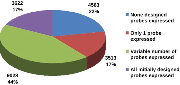
From the initial set of 103,000 probes, approximately half (51,661) were considered to be expressed, an expected low result that reflects the relatively complex tissue and species composition of the EST dataset that was assembled in the unigene set used to design the probes. For example, flower tissue was sampled and ESTs sequenced were represented in the unigene dataset. Transcripts specific to this tissue would most likely not be present in the xylem tissue used in this study. Nevertheless, expressed probes accounted for 78% (16,163) of the genes represented on the array, indicating that the number of expressed probes per gene varied considerably (Figure 1). Interestingly, even though the full transcripts would be theoretically present, for only 3,622 genes all the probes initially designed were consistently expressed, which might be a result of polymorphisms between the unigene probe sequence and the transcripts expressed by the parents (Figure 1). On the other extreme, almost the same amount of genes (3,513) had only one probe expressed and although this might partially be a consequence of the ad hoc expression cutoff threshold used that, if changed, could have excluded these probes or included more probes, it could also be the influence of developing microarray from complex EST libraries (Figure 1). For instance, it could be that several probes (four in this case) had a polymorphism between the unigene probe sequence and the transcripts expressed by the parents.
4563 22%
3513 17% 9028
44% 3622
17%
None designed probes expressed
Only 1 probe expressed
Variable number of probes expressed All initially designed probes expressed
Figure 1: Number of probes expressed per probeset compared to what was
initially designed on the screening microarray. A probe-level analysis of expression for the 20,726 unigenes considered probes not expressed when more than 90% of the individuals had signal below a background threshold.
4.2. Simultaneous detection and genotyping of SFPs in progeny data
The averaged, Log2 transformed, quantile-normalized data for the 96 individuals sampled were analyzed together to generate a gene-rich map of Eucalyptus based on SFPs anchored to microsatellites. Initially, the methods developed by Drost et al. [21] for genotyping SFPs in the highly heterozygous genome of poplar were applied to our dataset. Different from that work our dataset only involved progeny individuals so that the analysis was used to simultaneously identify and genotype SFPs. Working on a per-probe basis, the signal intensity of each individual offspring was assigned to either one of two distinct clusters using the k-means clustering learning algorithm. Using a chi-square test, probes showing a 1:1 pseudo-testcross segregation were selected. As SFP segregate as dominant markers probes segregating 3:1 were also selected. Although theoretically such probes could be segregating 1:2:1 (Figure 6D) the separation of the signal intensity into three clusters would be challenging and could result in higher proportions of genotype miscalls due to the expected overlap between signals from these classes. At a 2
1 . .f= d
> 0.05), 65% (28,304/43,777) of the probes displayed a Mendelian segregation ratio, with 12,148 segregating 1:1 and 16,156 segregating 3:1 (Table 1).
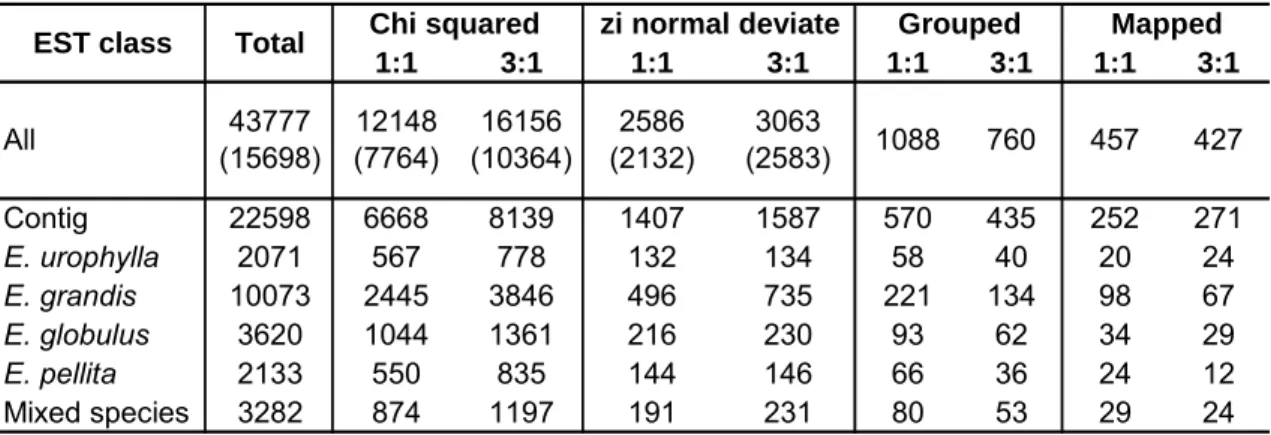
Table 1: Number of probes selected after applying the SFP detection and
mapping pipeline to the genotype dataset of 96 F1 individuals of the E. urophylla x E. grandis pedigree. Unigenes derived from a consensus sequence involving ESTs from different species are called Contigs, while singletons are listed by species. Number of unigenes represented is shown between parentheses.
The degree of separation between clusters was measured by calculating the probability of individuals assigned to one cluster being a member of the other cluster through a modified normal deviate zi (see methods). Individuals with zi equal to or smaller than 1.96 (P ≥ 0.05) are likely to overlap with the other cluster and were assigned as missing data to avoid genotype miscalls. Whenever an excessive number of individuals (more than 10%) were considered as miscall the probe was discarded. This selection step of the SFP detection pipeline is the most effective one as only 5,649 probes, representing altogether 4,300 unigenes were selected. A few genes (255) had more than two probes selected; an important result if one considers that the selection of fewer probes per probeset indicates detection of SFPs rather than GEMs. At this stage, the number of detected SFPs segregating 3:1 was slightly greater than that segregating 1:1, a pattern that was inverted after assigning these markers to linkage groups and stabilized after mapping and ordering them (Table 1).
1:1 3:1 1:1 3:1 1:1 3:1 1:1 3:1
Contig 22598 6668 8139 1407 1587 570 435 252 271
E. urophylla 2071 567 778 132 134 58 40 20 24
E. grandis 10073 2445 3846 496 735 221 134 98 67
E. globulus 3620 1044 1361 216 230 93 62 34 29
E. pellita 2133 550 835 144 146 66 36 24 12
Mixed species 3282 874 1197 191 231 80 53 29 24
457 427
2586 (2132)
3063
(2583) 1088 760
All 43777
(15698)
12148 (7764)
16156 (10364)
Although ESTs that grouped into contigs are usually referred to be of higher quality than those that did not group (singletons), we found only a borderline significant difference in the ability of probes derived from these two different types of unigenes to reveal SFPs ( 2
1 . .f= d
χ = 4.94 P = 0.0262) (Table 2). Although significant, this result indicates that singleton unigenes are a useful source of probes for SFP discovery.
Table 2: Association between the source of probes (contigs vs. singletons) and
the rate of SFP detection.
Contig Singleton Total
SFP Detected 2994 2655 5649
SFP Not detected 19604 18524 38128
Total 22598 21179 43777
2 1 . .f= d
χ = 4.94 P = 0.0262
Finally, to avoid redundant information the 5,649 probes revealing putative SFPs (2,586 segregating 1:1 and 3,063 segregating 3:1) were filtered to keep only one best SFP per gene for mapping. The selection criteria involved three steps (see methods). The first (pick probes with less missing data) intrinsically gives priority to probes with individuals well assigned to clusters; the second selects probes segregating 3:1 over those segregating 1:1 under the rationale that these markers are more informative because they segregate from both parents; and, the third step uses the gap calculated between clusters mean to minimize genotype miscalls due to overlapping. The resulting 4,300 selected SPFs, being 1,915 and 2,385 segregating 1:1 and 3:1, respectively, were used in the linkage mapping analysis (Table 1).
4.3. Construction of a gene-rich map for Eucalyptus
SFPs) represent unique genes while the remaining 180 markers are microsatellites. The microsatellites played an important role to confidently assign the SFPs to the expected 11 linkage groups of Eucalyptus formed at a minimum LOD of 7.0. A total of 1,848 SFPs grouped at this LOD threshold (Table 1) could, in principle, be ordered along the linkage groups. However a framework map with high likelihood support was constructed by simulated annealing, excluding markers that contributed to unstable marker orders. As microarray data is inherently noisy, we opted for map quality rather than allocating more genes but increasing the chance of erroneously ordering SFPs.
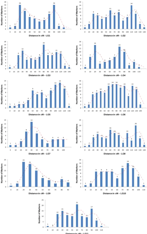
From the total number of SFPs mapped, 457 segregated 1:1 and 427 segregated 3:1, which received the acronym of BC and F2, respectively. The quality of the map is comparable to that generated by other classes of molecular markers, with markers evenly distributed throughout the linkage group. Except for a few cases on the edge of linkage groups, there were no evidences of major clustering or regions lacking genes (Figure 3), with SFPs spread equally along the intervals of microsatellites (Figure 2). However, some linkage groups had more (e.g. 6 and 8) genes mapped than others (e.g. 7), possibly resulting from a general greater abundance of genes on those chromosomes, or at least of those expressed in the transcriptome of differentiating xylem tissue (Table 3).
CL7781Cntig1_721_BC 0.0 CL2235Cntig1_1469_BC 1.4 CL1024Cntig1_716_F2 7.8 GR_SGTON3901_607_BC 10.2 CL8314Cntig1_423_BC 12.1 CL4444Cntig1_637_BC 12.2 CL795Cntig1_38_BC 15.3 CL334Cntig1_372_F2 PE_SGTON9383_309_BC 15.9 SP_SGTON10063_197_BC 16.3 GR_SGTON7616_409_F2 17.3 GR_SGTON5837_534_BC 17.4 en006 18.0 PE_SGTON9412_572_BC 18.3 UR_SGTON12007_309_BC 18.7 CL4375Cntig1_905_BC 19.0 CL1515Cntig1_859_F2 19.3 CL6793Cntig1_338_BC 19.4 CL6386Cntig1_256_F2 19.6 GR_SGTON2795_276_F2 20.2 CL478Cntig1_1430_BC 20.3 CL8441Cntig1_230_F2 20.6 CL2164Cntig1_724_F2 20.7 GR_SGTON5569_601_F2 20.8 SP_SGTON10760_330_F2 21.3 CL2954Cntig1_579_F2 23.4 CL2987Cntig1_844_F2 23.8 UR_SGTON11969_226_F2 24.7 CL4830Cntig1_524_F2 25.4 SP_SGTON11108_307_F2 27.6 CL7442Cntig1_522_BC 29.9 UR_SGTON12096_448_F2 31.2 CL1Cntig123_689_F2 CL760Cntig1_840_F2 31.3 embra983 34.4 CL7486Cntig1_61_F2 36.0 GR_SGTON6682_203_BC 36.8 UR_SGTON11867_438_F2 37.9 CL4884Cntig1_1051_BC 39.9 CL1917Cntig1_528_BC 42.0 CL6844Cntig1_317_BC 44.6 embra2000 44.9 CL547Cntig1_624_F2 47.0 GR_SGTON3599_68_BC 47.8 CL7736Cntig1_625_F2 48.4 embra180 49.8 UR_SGTON11845_307_F2 52.6 CL296Cntig1_673_F2 53.0 embra070 54.5 CL7537Cntig1_765_BC 56.5 SP_SGTON10371_609_BC 58.9 embra632 62.5 CL1414Cntig1_899_F2 63.2 embra012 65.8 CL4661Cntig1_1201_BC 66.6 CL6038Cntig1_271_F2 67.1 GL_SGTON49_262_BC 67.9 CL3339Cntig1_1350_BC 70.3 embra934 70.9 CL1242Cntig1_1575_BC 71.7 CL1409Cntig1_517_F2 73.7 GL_SGTON413_134_BC 73.8 CL2341Cntig1_1001_F2 74.3 CL70Cntig1_745_F2 74.5 embra1639 76.3 CL7148Cntig1_436_F2 76.5 GR_SGTON5303_312_F2 78.2 UR_SGTON12485_294_F2 80.5 CL1Cntig128_433_BC 81.1 CL2861Cntig1_771_F2 81.4 CL805Cntig1_513_F2 82.3 GR_SGTON7308_161_BC 82.7 CL6638Cntig1_1032_F2 82.9 CL1265Cntig1_668_BC 83.0 embra219 83.3 embra705 83.4 GR_SGTON4964_344_F2 83.5 CL7458Cntig1_796_BC 84.2 CL1146Cntig1_1116_BC 85.9 GL_SGTON1535_59_F2 86.5 GR_SGTON6697_790_BC 87.2 GL_SGTON1586_136_BC 88.4 GR_SGTON7172_279_F2 89.7 PE_SGTON9483_305_BC 90.7 CL5916Cntig1_862_BC 95.5 CL3272Cntig1_1198_BC 101.6 CL3949Cntig1_605_BC 0.0 GL_SGTON976_228_F2 2.9 embra058 8.1 embra068 9.2 GR_SGTON8849_179_BC 12.2 CL67Cntig1_382_BC 13.8 UR_SGTON11726_280_F2 CL4279Cntig1_402_BC 15.4 CL2077Cntig1_854_BC 16.5 GR_SGTON6994_535_F2 18.1 CL641Cntig1_809_F2 18.4 CL1598Cntig1_741_BC 18.8 CL667Cntig1_1601_F2 19.6 CL276Cntig1_274_F2 22.0 GR_SGTON3009_195_BC 23.4 SP_SGTON11263_206_F2 23.6 PE_SGTON9249_246_F2 24.9 GR_SGTON3408_302_BC 25.1 GR_SGTON1677_267_BC 27.3 UR_SGTON11683_344_BC 29.0 SP_SGTON11387_499_BC 29.6 GL_SGTON1487_650_BC 30.4 CL3595Cntig1_761_F2 31.9 GL_SGTON1088_142_F2 33.0 CL1119Cntig1_839_BC 36.9 CL3297Cntig1_637_BC CL6250Cntig1_396_BC 38.4 UR_SGTON11753_109_F2 41.1 CL576Cntig1_877_BC 41.3 embra063 42.1 GR_SGTON5829_271_BC 44.6 GR_SGTON6364_179_BC 45.7 embra126 48.2 embra043 49.4 embra1333 50.1 eg111 50.9 CL677Cntig1_713_F2 51.3 embra1332 51.5 SP_SGTON10198_594_F2 52.3 embra898 embra989 53.1 CL7027Cntig1_849_F2 54.7 embra915 58.9 CL7096Cntig1_510_BC 59.0 embra172 60.0 CL2206Cntig1_1131_F2 62.5 CL1181Cntig1_1082_F2 63.1 embra373 63.4 embra072 65.3 GL_SGTON1640_189_BC 65.8 embra390 66.0 CL356Cntig1_871_F2 67.5 GR_SGTON6910_278_F2 69.5 GR_SGTON8231_506_F2 71.9 GR_SGTON3197_239_F2 72.7 SP_SGTON10895_226_F2 73.2 GL_SGTON1270_256_F2 74.2 embra091 76.2 SP_SGTON10411_205_F2 76.5 CL1340Cntig1_687_F2 77.5 GR_SGTON1681_276_F2 77.7 CL4277Cntig1_791_F2 78.2 GR_SGTON6230_126_BC 78.8 CL5888Cntig1_375_F2 82.0 CL779Cntig1_417_F2 82.3 GR_SGTON8144_257_BC 83.9 GR_SGTON6460_222_F2 84.4 CL3171Cntig1_1242_BC 88.2 CL259Cntig1_353_F2 GR_SGTON8067_204_F2 92.4 CL1098Cntig1_503_BC 94.9 CL702Cntig1_1022_BC 95.3 CL1Cntig11_455_F2 97.0 GR_SGTON7550_475_BC 98.1 embra1369 98.6 GR_SGTON7479_216_F2 101.6 UR_SGTON12059_390_F2 102.0 UR_SGTON12257_208_F2 103.3 CL4381Cntig1_616_BC 103.8 GL_SGTON880_145_BC 105.5 CL2638Cntig1_490_F2 105.7 CL5352Cntig1_602_BC 106.6 UR_SGTON11762_297_F2 106.8 GR_SGTON7222_258_F2 107.1 GL_SGTON1456_404_BC 107.9 GL_SGTON453_194_BC 108.5 CL1656Cntig1_1097_F2 109.9 CL2256Cntig1_263_F2 CL1108Cntig1_1661_F2 110.0 SP_SGTON10560_259_F2 CL3773Cntig1_916_F2 CL1850Cntig1_1284_F2 CL5883Cntig1_311_F2 110.8 UR_SGTON11777_330_F2 111.7 CL1735Cntig1_850_F2 115.2 CL2019Cntig1_654_F2 117.5 CL765Cntig1_1358_BC 118.8 SP_SGTON11388_314_F2 119.4 UR_SGTON12233_365_BC 122.7 CL5633Cntig1_698_F2 124.7 GR_SGTON8154_343_BC 127.9 GL_SGTON753_314_BC 139.8 CL1Cntig18_662_BC 0.0 GL_SGTON220_290_BC 12.3 GR_SGTON3731_409_BC 13.9 embra1661 16.1 CL1341Cntig1_562_F2 16.7 CL3366Cntig1_1168_F2 18.2 GR_SGTON6791_235_F2 CL740Cntig1_640_F2 19.5 GR_SGTON5275_351_F2 19.7 CL2236Cntig1_1024_F2 19.9 CL3351Cntig1_774_F2 20.4 CL863Cntig1_1131_BC 20.7 GL_SGTON883_480_BC 21.1 CL2090Cntig1_907_BC 23.6 GR_SGTON6973_174_BC 23.7 CL1870Cntig1_514_F2 24.1 CL248Cntig1_992_BC 25.1 embra189 25.3 CL7569Cntig1_391_BC 26.3 PE_SGTON9263_122_F2 27.1 CL807Cntig1_457_BC 28.3 PE_SGTON9872_279_BC 29.5 CL399Cntig1_1184_F2 32.8 UR_SGTON11546_313_BC 33.2 PE_SGTON9106_199_BC 37.7 GR_SGTON7525_457_BC 38.7 CL3247Cntig1_992_F2 39.0 GR_SGTON7627_145_BC 39.9 GR_SGTON2158_213_BC 40.1 CL265Cntig1_1110_F2 40.9 CL1407Cntig1_1084_BC 44.7 SP_SGTON10418_526_BC 45.7 CL3469Cntig1_624_BC 47.0 CL1826Cntig1_1412_F2 48.8 CL1520Cntig1_829_BC 49.4 SP_SGTON10177_303_BC 50.2 GR_SGTON7504_694_F2 52.1 CL1000Cntig1_434_F2 52.7 CL3810Cntig1_375_BC 55.6 GL_SGTON457_414_BC 57.8 CL1869Cntig1_862_F2 59.2 UR_SGTON11986_460_BC 60.3 CL5029Cntig1_622_BC 60.6 CL1597Cntig1_1105_F2 62.5 GL_SGTON1029_277_F2 63.3 SP_SGTON10982_330_BC 65.2 GR_SGTON5535_149_F2 65.8 CL1332Cntig1_1062_F2 68.1 SP_SGTON10236_416_BC 69.1 CL1859Cntig1_1021_BC 70.3 UR_SGTON12487_451_BC 70.8 CL5417Cntig1_762_BC 71.4 embra122 71.7 CL3533Cntig1_993_F2 72.1 embra239 72.5 embra361 73.3 embra350 74.0 CL102Cntig1_490_F2 74.2 CL696Cntig1_481_BC 74.4 PE_SGTON8890_175_BC 78.3 CL978Cntig1_504_BC 78.4 GL_SGTON1564_597_BC 78.5 eg098 78.8 CL1445Cntig1_697_F2 79.1 GR_SGTON5055_368_F2 79.8 embra1656 80.4 embra286 82.0 PE_SGTON9655_298_BC 82.6 embra1007 84.0 CL341Cntig1_1501_BC 86.6 CL3851Cntig1_652_F2 87.5 CL3195Cntig1_528_BC 88.8 GR_SGTON3243_221_BC 89.1 CL3005Cntig1_744_BC 89.8 GR_SGTON1920_293_BC 90.5 embra125 90.7 GR_SGTON4942_297_F2 93.5 CL1459Cntig1_858_BC 95.1 CL7585Cntig1_1161_F2 95.2 CL2037Cntig1_891_BC 98.8 CL2105Cntig1_786_F2 99.3 SP_SGTON10357_364_F2 99.4 CL62Cntig1_400_BC 99.7 GR_SGTON6941_318_BC 100.6 SP_SGTON11176_310_BC 101.1 CL5820Cntig1_388_F2 103.0 CL176Cntig1_859_BC 103.3 CL4326Cntig1_222_F2 104.0 CL2078Cntig1_1045_F2 104.1 CL2846Cntig1_148_BC 106.1 SP_SGTON10945_481_BC 106.5 CL498Cntig1_1522_F2 106.7 GR_SGTON2724_412_BC 106.8 GR_SGTON2800_226_BC 109.3 GR_SGTON7089_704_F2 110.3 GR_SGTON5628_47_F2 110.5 CL971Cntig1_1683_BC 111.2 embra1494 112.8 CL1142Cntig1_547_F2 113.3 GL_SGTON1050_469_F2 114.5 SP_SGTON10534_690_F2 115.9 GR_SGTON7143_699_F2 116.8 CL1798Cntig1_885_BC 117.8 CL3778Cntig1_737_BC 118.4 CL1083Cntig1_917_BC 124.6 PE_SGTON9906_279_BC 126.6 GR_SGTON7770_695_BC 133.9 CL346Cntig1_1103_BC 0.0 UR_SGTON12172_141_F2 9.0 SP_SGTON10390_101_BC 10.7 GL_SGTON1204_225_BC 12.8 GR_SGTON3348_246_BC 13.4 GL_SGTON498_391_F2 15.7 CL2145Cntig1_810_BC 17.3 CL4673Cntig1_1191_BC 23.5 CL3678Cntig1_335_F2 25.7 embra186 27.3 CL5936Cntig1_711_F2 27.8 GL_SGTON200_203_BC 28.4 CL7354Cntig1_489_BC 29.1 CL502Cntig1_711_F2 30.7 CL3959Cntig1_783_BC 31.0 CL5886Cntig1_420_BC 31.1 embra1122 32.2 embra078 33.8 CL5143Cntig1_418_BC 34.6 CL5682Cntig1_116_BC 34.9 CL5375Cntig1_150_F2 35.0 CL1147Cntig1_827_F2 CL5652Cntig1_577_F2 36.4 embra004 37.6 SP_SGTON10213_578_F2 40.9 CL2703Cntig1_726_F2 41.3 CL559Cntig1_1038_BC 42.3 CL287Cntig1_977_BC UR_SGTON11720_166_BC 42.7 embra1507 43.4 CL5506Cntig1_699_BC 43.7 GR_SGTON6800_380_BC 44.3 embra1144 44.9 embra332 46.5 embra645 48.0 embra1944 50.6 GR_SGTON6809_535_BC 52.8 CL5242Cntig1_483_BC 56.3 GR_SGTON6879_444_F2 57.0 SP_SGTON10335_87_F2 61.5 CL4128Cntig1_597_BC 62.4 CL79Cntig1_586_F2 63.0 CL415Cntig1_929_F2 63.8 CL1945Cntig1_26_BC 66.3 GR_SGTON7147_181_BC 70.2 eg128 72.2 CL410Cntig1_1305_BC 78.7 CL7723Cntig1_315_BC 80.5 CL2904Cntig1_603_F2 82.8 embra179 85.2 CL264Cntig1_803_BC 85.3 embra036 87.1 GL_SGTON456_89_BC 88.3 CL6345Cntig1_473_F2 89.4 SP_SGTON10080_230_BC 89.9 CL1377Cntig1_1258_F2 CL2027Cntig1_990_BC 90.6 GR_SGTON3760_479_BC 91.2 CL450Cntig1_1852_F2 91.6 CL4509Cntig1_652_F2 GL_SGTON489_442_F2 92.6 UR_SGTON12362_344_BC 92.7 CL2694Cntig1_714_BC 93.4 CL284Cntig1_658_BC 93.5 GR_SGTON7660_413_BC 94.1 CL834Cntig1_988_BC 95.0 CL4683Cntig1_1182_BC 96.1 CL90Cntig1_735_BC 97.7 SP_SGTON10142_390_BC 99.9 GR_SGTON6535_402_F2 101.4 CL2976Cntig1_823_BC 103.5 LG 1 LG 2 LG 3 LG 4
Figure 2: High-density SFP/microsatellite genetic linkage map of E. urophylla x
Figure 3: Frequency distribution of SFPs along the extension of the eleven linkage groups indicating variable marker clustering patterns.
1 2 16 12 8 7 5 6 10 16 2 1 0 2 4 6 8 10 12 14 16 18
0 10 20 30 40 50 60 70 80 90 100 110
N u m b er o f M ar ker s
Distance in cM - LG1
1 3 9 8 6 7 11 8 10 5 7 14 9 3 1 0 2 4 6 8 10 12 14 16
0 10 20 30 40 50 60 70 80 90 100 110 120 130 140
N u m b er o f M ar ker s
Distance in cM – LG2
1 0
9 12
6 7 6 8 16 9 9 11 10 2 1 0 2 4 6 8 10 12 14 16 18
0 10 20 30 40 50 60 70 80 90 100 110 120 130 140
N u m b er o f M ar ker s
Distance in cM – LG3
1 7 14 3 4 5 7 13 10 2 4 1 0 2 4 6 8 10 12 14 16
0 10 20 30 40 50 60 70 80 90 100 110
N u m b er o f M ar ker s
Distance in cM – LG4
1 1 2 2 4 9 7 8 5 9 12 13 10 1 0 2 4 6 8 10 12 14
0 10 20 30 40 50 60 70 80 90 100 110 120 130
N u m b er o f M ar ker s
Distance in cM – LG5
1 2 8 9 10 9 13 14 14 12 13 7 13 11 2 0 2 4 6 8 10 12 14 16
0 10 20 30 40 50 60 70 80 90 100 110 120 130 140
N u m b er o f M ar ker s
Distance in cM – LG6
1 1 3 8 13 7 4 2
4 4 4
0 2 4 6 8 10 12 14
0 10 20 30 40 50 60 70 80 90 100
N u m b er o f M ar ker s
Distance in cM – LG7
1 2 9 12 9 8 16 13 11 4 13 6 20 8 2 0 5 10 15 20 25
0 10 20 30 40 50 60 70 80 90 100 110 120 130 140
N u m b er o f M ar ker s
Distance in cM – LG8
1 3 23 21 15 8 6 3 7 4 0 5 10 15 20 25
0 10 20 30 40 50 60 70 80 90
N u m b er o f M ar ker s
Distance in cM – LG9
1 2
9 9 9 9
5 11 14 11 6 1 0 2 4 6 8 10 12 14 16
0 10 20 30 40 50 60 70 80 90 100 110
N u m b er o f M ar ker s
Distance in cM – LG10
1 0 12 15 11 10 21 10 9 17 6 1 0 5 10 15 20 25
0 10 20 30 40 50 60 70 80 90 100 110
N u m b er o f M ar ker s
Linkage Group SSR Genes Total Length (cM)
Intermarker distance (cM)
Mean
Std Deviation
LG1 11 75 86 102 1.20 1.25
LG2 17 85 102 140 1.38 1.55
LG3 12 95 107 134 1.26 1.63
LG4 12 59 71 103 1.48 1.59
LG5 23 61 84 124 1.49 1.76
LG6 34 104 138 136 0.99 0.97
LG7 14 37 51 98 1.96 1.89
LG8 12 122 134 134 1.01 1.16
LG9 16 75 91 88 0.98 1.06
LG10 16 71 87 108 1.25 1.45
LG11 13 100 113 110 0.98 1.55
Total markers mapped 180 884 1064 1275 1.21 1.44
Table 3: Descriptive statistics for the 11 linkage groups of the
SFP/microsatellite map.
Although some linkage groups had more microsatellites than others, this apparently did not influence the amount of SFPs mapped. For example, linkage group 7 has 14 microsatellites and only 37 genes were assigned to this group; whereas linkage group 8, which has 12 microsatellites, was complemented with SFPs for 122 genes (Table 3). This lack of pattern is consistent across the whole map, suggesting that SFPs are behaving independently from the microsatellites and can in fact contribute to map saturation.
employing an experimental design that allows for the detection of SFPs segregating 3:1 seems to be the best one not only as it allows mapping a larger number of genes but also because the final map quality is substantially increased.
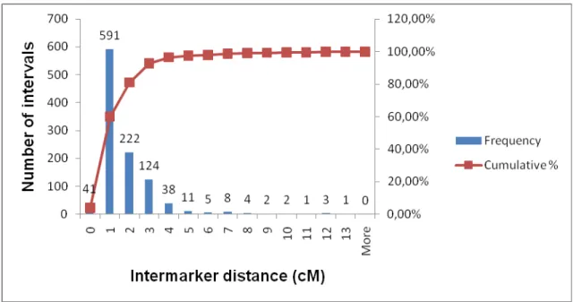
Figure 4: Frequency histogram showing the distribution of intervals between
Table 4: Contribution of SFPs segregating 3:1 to map quality. Number of markers mapped and final linkage group length for each linkage group are shown when (i) mapping microsatellites plus SFPs segregating 1:1 (Only 1:1), (ii) microsatellites plus SFPs segregating 3:1 (Only 3:1) and (iii) microsatellites plus SFPs segregating for both patterns (Both).
# markers Length (cM) # markers Length (cM) # markers Length (cM)
LG 1 45 146 66 92 86 102
LG 2 73 168 70 136 102 140
LG 3 78 208 44 87 107 134
LG 4 59 151 40 67 71 103
LG 5 59 244 63 122 84 124
LG 6 87 197 98 125 138 136
LG 7 39 98 42 109 51 98
LG 8 84 149 81 116 134 134
LG 9 66 138 61 87 91 88
LG 10 73 182 48 88 87 108
LG 11 75 164 66 101 113 110
Total 738 1845 679 1130 1064 1275
Only 1:1 Only 3:1 Both
Linkage Group
4.4. SFP identification using mixed-model analysis of variance
Next, we were interested to know whether it would be possible to recover the mapped SFPs by doing a detection analysis on the data from the screening experiment where only the 28 biologically replicated individuals were used. Wolfinger et al. [50] and Rostoks et al. [16] previously proposed that fitting microarray data to a mixed-model analysis of variance is an effective way to separate the sources of variation and test the significance of these effects, identifying differentially expressed genes and putative SFPs, respectively. We expanded this principle and hypothesized that the same analysis could be used on our progeny data.
methods). Significance of this source of variation would indicate genes where the signal intensity of one (or more) probe(s) deviates from the probeset’s mean in a genotype dependent fashion, which is exactly the definition of a SFP. However, keep in mind that this analysis does not determine which probe of the probeset is behaving as an SFP. After correcting the significance threshold of the F tests for multiple testing, 4,648 genes showed significant GP effect at a false discovery rate < 0.005 (P < 0.0022), represented by a total of 25,600 probes.
This selection using ANOVA recovered 87% (1,603) of the genes that were linkage grouped when the full dataset from the 96 individuals was used (Figure 5A). When considering only genes that were represented by probes ultimately mapped, a fewer proportion was left aside and 811 (92%) genes were common to both selections (Figure 5B). These results indicate that using a mixed-model ANOVA on microarray data is a valid approach to identify genes with the source of variation of interest significant, even when a complex progeny dataset is being used.
As ANOVA does not determine which probe of the probeset is the putative SFP, we searched within each ANOVA-selected probeset for candidate SFPs applying the k-means clustering previously described to assign the normalized data of the 28 individuals into two distinct clusters. The chi square analysis of segregation and the modified normal deviate (zi) were also calculated to distinguish well separated clusters with 1:1 and 3:1 proportions from non-informative probes.
3045 1603
(87%) 245
Genes selected by ANOVA
Genes previously grouped
A
3837 (92%)811 73
Genes selected by ANOVA
Genes previously mapped
B
2687 1564
(85%) 284
Genes kept after selection within gene
Genes previously grouped
C
3454 797
(90%) 87
Genes kept after selection within gene
Genes previously mapped
C
Figure 5: Venn diagrams comparing efficiency of identifying SFPs using
mixed-model ANOVA on dataset from 28 individuals. A) Genes with significant GP effect compared to linkage grouped genes from the reference map. B) Genes with significant GP effect compared to mapped genes from the reference map. C) Genes that were still selected after further within gene selection compared to linkage grouped genes from the reference map. D) Genes that were still selected after further within gene selection compared to mapped genes from the reference map. Values between parentheses refer to the percentage of the genes linkage grouped or mapped that were common between analyses.
Assuming that probes which were assigned to linkage groups after our analysis involving 96 individuals are the real SFPs, the number of false positives detected by ANOVA was relatively low (5,917 probes in 2,687 genes). Those probes probably represent spurious segregation that were later removed when the number of individuals increased from 28 to 96. At any rate, it is noticeable that this approach confidentially retrieved the information generated using a much larger number of individuals (28 versus 96) and can be confidentially used during the screening step.
4.5. Number of probes per probeset
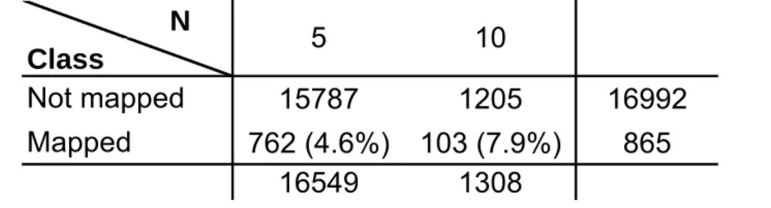
density oligonucleotide array. Nevertheless, because it was not known how many probes would be necessary to have at least one able to discover an SFP into the gene, for a subset of 1,308 genes, corresponding to 6.3% (1,308/20726) of the available unigene set, a probeset with a total of 10 probes was designed (Additional file 2).
Table 5 compares the relative efficiency of SFP discovery when five or 10 probes are used per probeset. A total of 4.6% of the genes with five probes designed had at least one SFP discovered and ultimately mapped on the reference map. In contrast, when 10 probes were used for the SFP screening and discovery experiment, the efficiency was almost doubled, increasing to 7.9%. A chi-squared test of homogeneity confirmed that this difference is highly significant (χd2.f.=1 =28;P<0.00001) clearly indicating that using more probes per
unigene does result in a significantly increased probability of discovering a segregating and mappable SFP and ultimately positioning the gene on the linkage map.
Table 5: Association between the number of probes screened for a gene (N)
and the number of genes ultimately mapped.
The percentage of genes mapped when N= 5 and 10 is shown in parenthesis.
Even though we had 2,868 other genes with a variable number between one and four probes designed (Additional file 2), we did not include them in the analysis because this number of probes was not intentionally designed. Rather, they ended up having a smaller number of probes selected per probeset because the remaining probes were not considered high quality according to