Testing the transferability of regression equations derived from small sub-catchments to a large area in central Sweden

Testing the transferability of regression equations derived from

small sub-catchments to a large area in central Sweden

Chong-yu Xu

1,2

1_{Department of Earth Sciences, Hydrology, Uppsala UniversityVillavagen 16, 75236 Uppsala, Sweden} 2_{Nanjing Institute of Geography and Limnology, Chinese Academy of Science}

E-mail: Chong-yu.Xu@hyd.uu.se

Abstract

There is an ever increasing need to apply hydrological models to catchments where streamflow data are unavailable or to large geographical regions where calibration is not feasible. Estimation of model parameters from spatial physical data is the key issue in the development and application of hydrological models at various scales. To investigate the suitability of transferring the regression equations relating model parameters to physical characteristics developed from small sub-catchments to a large region for estimating model parameters, a conceptual snow and water balance model was optimised on all the sub-catchments in the region. A multiple regression analysis related model parameters to physical data for the catchments and the regression equations derived from the small sub-catchments were used to calculate regional parameter values for the large basin using spatially aggregated physical data. For the model tested, the results support the suitability of transferring the regression equations to the larger region.

Key words: water balance modelling, large scale, multiple regression, regionalisation

Introduction

A capability to simulate river flows in large river basins is desirable for at least four reasons (Arnell, 1999). Firstly, for operational and planning purposes, water resource managers need to estimate the spatial variability of resources over the regions for which they are responsible, at a spatial resolution finer than can be provided by observations alone. Secondly, hydrologists and water managers are concerned about the effects of land-use changes and climatic variability over large geographic domains. Thirdly, hydrological models are useful in estimating point and non-point sources of pollution loading to streams. Fourthly, hydrologists and atmospheric modellers are aware of weaknesses in the representation of hydrological processes in regional and global atmospheric models.

The development of simulation models in hydrological research has focused mainly on basins smaller than 2000 km2 _{and on their extrapolation to ungauged catchments or}

regions, by estimating the parameters of the models from only the physical characteristics of the catchments. Nash and Sutcliffe (1970) stated: “few hydrologists would

318

of view, the full benefit of a conceptual model will be realised only to the extent that it is possible to synthesise data for ungauged catchments. It is therefore appropriate to continue research in this aspect”.

During the last decade, the evolution of continental-scale hydrology for water resources assessment at large scales and for improvements in the representation of land-surface hydrological processes in regional and global atmospheric models has placed new demands on hydrological modellers. How to derive model parameter values from spatial data sets without calibrating the model at the large scale is the key to the development and application of macro-scale hydrological models. Moreover, new models working on rectangular grids at large scales makes regionalisation even more difficult, because their calibration over a large area is simply not feasible. In previous applications of large-scale hydrological models, all or part of the parameters have been determined in one of the following ways: (1) fixed globally at ‘reasonable values’, or values selected from the literature for the appropriate land cover or from previous studies. (Wood et al., 1992; Stamm et al., 1994; Nijssen et al., 19970; Arnell, 1999; Ma et al., 2000), (2) calibrate the model on a number of catchments and regional parameters are obtained by interpolation (Guo et al., 2001; Gottschalk et al., 2001), (3) direct estimation from physical data for some parameters and calibration for the others (Watson et al., 1999) and (4) develop multiple regression equations that relate physical characteristics to model parameters optimised on the sub-catchments selected, and use the equations to estimate model parameters for the grid cell in the large area (Abdulla and Lettenmaier, 1997a, b; Kite, 1994). The difference in transferring the regression equations from small sub-catchments to large basins must be quantified.

Here, the suitability of transferring regression equations from sub-catchments to the larger region for estimating model parameters has been investigated in an application of a conceptual snow and water balance model to a seasonally snow-covered region in central Sweden. The model was optimised on all the sub-catchments in the region and multiple regression equations relating model parameters to physical catchment data were established; parameter values, calculated from the regression equations using spatial physical data for all the sub-catchments, were compared with the optimised values. From the regression equations for the small sub-catchments, regional parameter values for the large basin were calculated using spatially aggregated physical data. These calculated values were then compared with optimised regional parameters using inputs of spatially aggregated hydrological data from the whole region. Finally, the regional water balance components simulated using parameter sets determined with different approaches were

compared and the differences caused by the transfer of regression equations from small to large scale were evaluated.

The water balance model

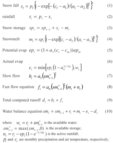
NOPEX-6 (Xu et al., 1996) is a typical water and snow balance model, developed for water balance investigations for the NOPEX (Halldin et al., 1998) area and Nordic region. Earlier versions of the model have been applied to over 100 catchments in more than 20 countries (Xu, 1992; Vandewiele et al., 1992; Vandewiele and Ni-Lar-Win, 1998; Müller-Wohlfeil, et al., 2003). The principal equations of NOPEX-6 are presented in Table 1. The input data to the model are monthly values of areal precipitation, long-term monthly average potential evapotranspiration and air temperature. Precipitation p_t is first divided into rainfall r_t and snowfall s_t by a temperature index function; at the end of each month snowfall is added to the snowpack sp_t, of which a fraction m_t melts and contributes to the soil moisture storage sm_t.

Table 1. Principal equations of the MWB-6 monthly snow and water balance model.

Snow fall ₌

{

₋

_[

₋

₍

₋

_{) (}

₋

₎

_]

2

}

+

2 1 1 / exp

1 c a a a

p

s_{t t t} (1)

rainfall rt = pt −st (2)

Snow storage spt = spt−1 +st −mt (3)

Snowmelt m_t =sp_t

{

1−exp

_[

₍

c_t −a₂

_{) (}

/ a₁−a₂

₎

_]

2

}

+ (4)

Potential evap ept =(1+a c3( t−cm))epm (5)

Actual evap

(

)

[

]

et ept a w

w ep t

t t

=min − / ,

1 4

(6)

Slow flow

(

)

2

1 5

+ −

= t

t a sm

b (7)

Fast flow equation ft =a

(

smt

)

(

mt+nt

)

+ −

2 1

6 (8)

Total computed runoff d_t =b_t +f_t (9)

Water balance equationsm_t =sm_t−1+r_t +m_t −e_t −d_t (10)

where: _wt =_rt +_smt+₋₁ is the available water; sm_t− sm_t

+

− =

1 max( 1, )0 is the available storage; nt rt ept e

r ept t

= − (1− − / )is the active rainfall;

p

_t and c_t are monthly precipitation and air temperature, respectively;

ep_m and

c

_m are long-term monthly average potential evapotransp-iration and air temperature, respectively; _{a i}

Parameters a₁ and a₂ are threshold temperatures which determine the form of precipitation and the rate of snowmelt. Before the rainfall contributes to the soil storage as ‘active’ rainfall, a small part is subtracted and added to the loss by evapotranspiration. The soil water storage contributes to evapotranspiration e_t, to the fast component of flow f_t and to slow flow s_t. The parameter a₃, used to convert long-term average monthly values to actual values of monthly potential evapotranspiration, can be eliminated from the model if potential evapotranspiration data are available or calculated using other methods. Parameter a₄ determines the actual evapotranspiration that is an increasing function of potential evapotranspiration and available water. The smaller the values for a₄, the greater the evaporation losses at all moisture storage states. The slow flow parameter a₅ controls the proportion of runoff that appears as ‘base flow’; higher values of a₅ produce a greater proportion of ‘base flow’. Values are expected to be higher in forest areas than in open fields and in sandy rather than clayey soils. The fast flow parameter a₆increases with the degree of urbanisation, average basin slope and drainage density; lower values are likely for catchments dominated by forest.

Study region and data

The study area is located in central Sweden — the basin of Lake Mälaren with a drainage area of about 30 000 km² which is in the order of one grid cell size in GCM modelling (Fig. 1). The area has 30 sub-catchments ranging in size from 6 to 4000 km2 _{and is one of the largest catchments in}

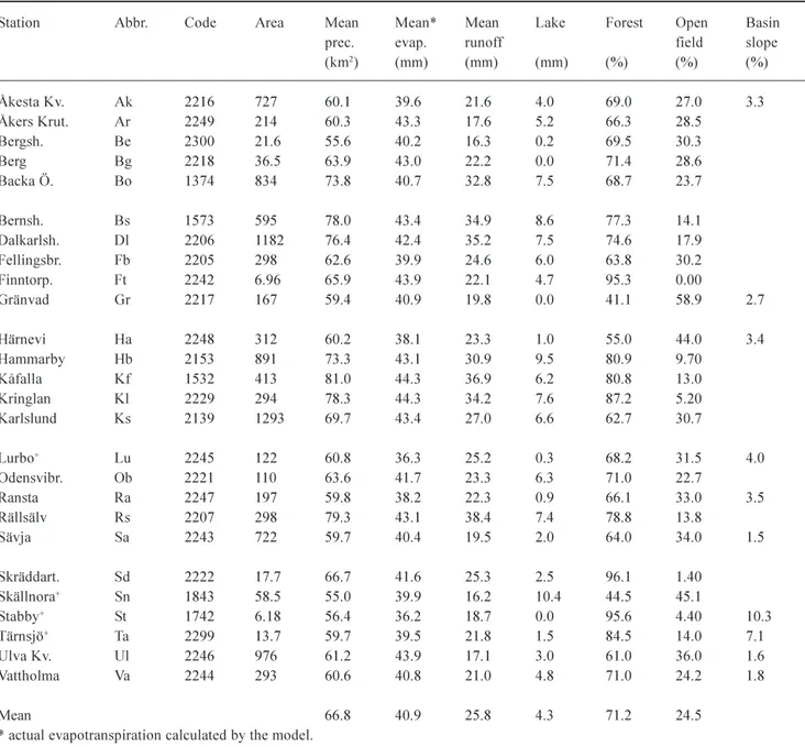
Sweden. The available data comprise at least 10 years’ daily precipitation from 41 stations and daily temperature from 12 stations. Land-use data are also available for the corresponding catchments. Of the 30 sub-catchments, only 26 of them have been used in this study, because earlier investigations (Seibert, 1995) indicated uncertainties in the water divides of four of the sub-catchments.

The landscape of the area is dominated by large lakes and plains separated by high undulating ridges, rich in faults. The geology is characterised by granites in the northeast, sedimentary gneisses in the south and leptites and hälleflintas in the northwest with some small granite-dominated areas. The northwest is mostly afforested (69.3%), while meadow and grain cultivation is predominant in the south (25%). Seibert (1995) and Garcia (1997) have shown that the distribution of soil type parallels the landuse, i.e., areas of forest generally consist of sandy soil, whereas agricultural areas consist of clay soil. The mean annual precipitation and discharge are 800 and 310 mm, respectively. Excluding Lake Mälaren itself, 5.7% of the area is lakes (Table 2.)

Fig.1. Map of Sweden with the locations of study region and NOPEX region.

TA FT

FB KL

RS

Lake Mälaren

SD AK

HA RA

BG

UL VA

SA

BE

SN

AR KF

DL

HB

BS LU

ST

OB

KS

BO

GR

0 20 40 km

N

Stockholm

1

2

320

Table 2. The hydrological and land-use data of the study region

Station Abbr. Code Area Mean Mean* Mean Lake Forest Open Basin

prec. evap. runoff field slope

(km2_{)(mm)(mm)(mm)(%) (%) (%)}

Åkesta Kv. Ak 2216 727 60.1 39.6 21.6 4.0 69.0 27.0 3.3

Åkers Krut. Ar 2249 214 60.3 43.3 17.6 5.2 66.3 28.5

Bergsh. Be 2300 21.6 55.6 40.2 16.3 0.2 69.5 30.3

Berg Bg 2218 36.5 63.9 43.0 22.2 0.0 71.4 28.6

Backa Ö. Bo 1374 834 73.8 40.7 32.8 7.5 68.7 23.7

Bernsh. Bs 1573 595 78.0 43.4 34.9 8.6 77.3 14.1

Dalkarlsh. Dl 2206 1182 76.4 42.4 35.2 7.5 74.6 17.9

Fellingsbr. Fb 2205 298 62.6 39.9 24.6 6.0 63.8 30.2

Finntorp. Ft 2242 6.96 65.9 43.9 22.1 4.7 95.3 0.00

Gränvad Gr 2217 167 59.4 40.9 19.8 0.0 41.1 58.9 2.7

Härnevi Ha 2248 312 60.2 38.1 23.3 1.0 55.0 44.0 3.4

Hammarby Hb 2153 891 73.3 43.1 30.9 9.5 80.9 9.70

Kåfalla Kf 1532 413 81.0 44.3 36.9 6.2 80.8 13.0

Kringlan Kl 2229 294 78.3 44.3 34.2 7.6 87.2 5.20

Karlslund Ks 2139 1293 69.7 43.4 27.0 6.6 62.7 30.7

Lurbo+ _{Lu 2245 122 60.8 36.3 25.2 0.3 68.2 31.5 4.0}

Odensvibr. Ob 2221 110 63.6 41.7 23.3 6.3 71.0 22.7

Ransta Ra 2247 197 59.8 38.2 22.3 0.9 66.1 33.0 3.5

Rällsälv Rs 2207 298 79.3 43.1 38.4 7.4 78.8 13.8

Sävja Sa 2243 722 59.7 40.4 19.5 2.0 64.0 34.0 1.5

Skräddart. Sd 2222 17.7 66.7 41.6 25.3 2.5 96.1 1.40

Skällnora+ _{Sn 1843 58.5 55.0 39.9 16.2 10.4 44.5 45.1}

Stabby+ _{St 1742 6.18 56.4 36.2 18.7 0.0 95.6 4.40 10.3}

Tärnsjö+ _{Ta 2299 13.7 59.7 39.5 21.8 1.5 84.5 14.0 7.1}

Ulva Kv. Ul 2246 976 61.2 43.9 17.1 3.0 61.0 36.0 1.6

Vattholma Va 2244 293 60.6 40.8 21.0 4.8 71.0 24.2 1.8

Mean 66.8 40.9 25.8 4.3 71.2 24.5

* actual evapotranspiration calculated by the model.

+ _{Catchments used for independent testing of the regression equations}

Approaches of parameters estimation

PARAMETER ESTIMATION FOR INDIVIDUAL

SUB-CATCHMENTS

Parameter values for individual sub-catchments are estimated in two ways:

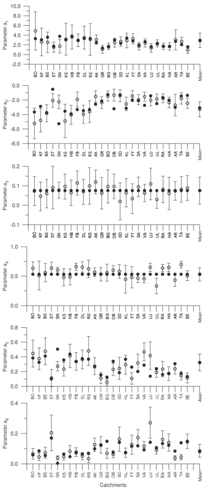
l Firstly, the model was calibrated on all 26 sub-catchments using an automatic optimisation method (Xu et al., 1996; Xu, 2001). The optimised parameter values and their 95% confidence intervals are shown in Fig.2.

l Secondly, the regression equations relating the optimised parameter values to physical properties of the catchments were developed using 22 randomly selected sub-catchments. The four remaining catchments were used to verify the equations.

In Table 3, the regression equations are shown with their values of R2_{. The verification using the four independent}

Catchments

0.0 0.2 0.4

P

a

ra

m

e

te

r a

6

M

ean

0.0 0.2 0.4 0.6 0.8

Par

a

m

e

te

r a

5

Me

a

n

0.0 0.5 1.0

Par

a

met

e

r a

4

Me

a

n

Catchments -2.0

0.0 2.0 4.0 6.0 8.0 10.0

Pa

ra

met

e

r a

1

Mean

-0.1 0.0 0.1 0.2

Pa

ra

m

e

te

r a

3

Me

an

Catchments

-8.0 -6.0 -4.0 -2.0 0.0

P

a

ram

e

ter a

2

Me

an

322

the sub-catchments are also given in Fig.2. For most catchments, the parameter values thus estimated lie in the 95% confidence interval of the optimised values. For parameters

a

₃ and

a

₄, the regional average values calculated from optimised values are used in the second approach, because: (i) these parameters are nearly constant over the region (Fig. 2); (ii) these parameters are the least sensitive compared to the others (Xu, 2001); and (iii) no significant regional regression equations could be found for them (Xu, 1999b).

ESTIMATION OF REGIONAL PARAMETERS

In this study, the Lake Mälaren basin, of the order of a GCM’s grid size, was considered to be a large catchment compared to its 30 sub-catchments. The parameter values for the large catchment were determined in two approaches.

l Firstly, the physical properties of the large catchment were determined and the regional model parameters were estimated using the regression equations developed for individual sub-catchments. (Table 4). l Secondly, the input data file of the large catchment was

assembled using the measurements of precipitation at 41 stations and of temperature at 12 stations in the area. For potential evapotranspiration, the monthly long-term

average values from Uppsala Flygplats station were used recursively to form a 10-year sequence concurrent with precipitation and temperature for the study region. The real-time series of the monthly potential evapotranspiration was calculated as an internal series using Eqn. (5) in Table 1. To produce a benchmark parameter set for comparison with the parameters determined from the regression equations, the model was calibrated on the large basin and the parameter values were optimised (Table 4).

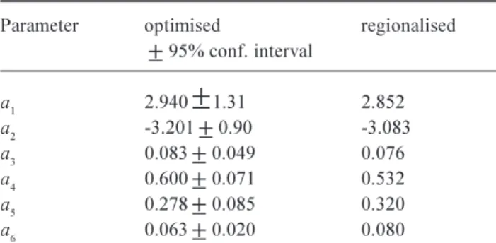
Because the parameter values determined from the regression equations are in the 95% confidence interval of the optimised values, the suitability of transferring the regression equations to the larger region is warranted.

Regional water balance simulation

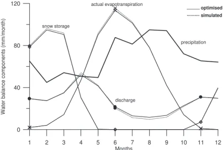
Water balance simulations for large catchments consist of three stages: determining regional model parameters from spatial data sets; defining input data; validation of model performance and parameter determination approach.

The regional model parameters and the input data set for the large catchment defined earlier are used here to simulate its water balance and the performance of the model in simulating discharges has been evaluated using the Nash-Sutcliffe (1970) efficiency criterion, R2_{. The simulated}

and observed monthly discharges for the Lake Mälaren basin are presented in Fig. 3; the R2 _{value between simulated and}

observed discharge is 0.87. Unfortunately, observations of actual evapotranspiration and of snowpack are not available for comparing with the simulated values. To provide a benchmark series for comparison, these data series were obtained by calibrating the model directly on the whole basin and comparing the results with the simulations. Figure 4 compares the calibrated and simulated regional time series of mean monthly discharge, actual evapotranspiration and snowpack. As expected from the comparison of regional parameter values given in Table 4, the model performed equally well in simulating regional water balance using regional parameters determined from regression equations and using optimisation. To provide a quantitative Table 3. Regression equations and coefficients R2

a₁ =.106 +.0229´Lake% + .000695´Forest (sandy soil)% R2_=0.80

a₂ = -.0395 - .0340´Lake% - .00297´open-field (clayey soil)% R2_=0.66

a₅ = .0949 + .0350´Lake% + .0010´open-field (clayey soil)% R2_=0.76

a₆ = .085 - .0116´Lake% + .000889´Forest (sandy soil)% R2_=0.72

Table 4. Regionalised and optimised regional parameter values together with their 95% confidence interval

Parameter optimised regionalised

±

95% conf. interval

a

1 2.940

±

1.31 2.852

a

2 -3.201

±

0.90 -3.083

a

3 0.083

±

0.049 0.076

a

4 0.600

±

0.071 0.532

a

5 0.278

±

0.085 0.320

a

6 0.063

±

0.020 0.080

Note: parameters a

5 and a6 are scaled up by 1000 and 10 000,

comparison, the percentage error in mean monthly values, ERR% was computed as

100

%= − ×

cal cal sim

X X X

ERR ₍₁₁₎

and used to evaluate the performance of the model in simulating mean monthly water balance components. The ERR% values for discharge, actual evapotranspiration and snowpack are -1.22%, 0.07% and 1.95%, respectively.

Discussion and conclusions

The transferability of regression equations from small sub-catchments to a large basin and/or to GCM/RCM rectangular grid cells is important if hydrological models are to be applied to large areas for water balance calculations of

0 12 24 36 48 60 72 84 96 108 120

Time in month

0 25 50 75 100

D

is

c

harg

e

in m

m

/m

onth

Observed _______ Regionalised

Fig. 3. Observed and simulated Lake Mälaren basin’s discharge with regionally regressed parameters

1 2 3 4 5 6 7 8 9 10 11 12

Months 0

40 80 120

Wa

te

r

b

a

la

nc

e c

o

m

pon

en

ts

(

m

m

/m

o

n

th)

precipitation

discharge snow storage

_____ optimised ... simulated

actual evapotranspiration

Fig. 4. Optimised and simulated mean monthly water balance of the Lake Mälaren basin with regional parameters

present climate and changing climate. In the absence of benchmark values of model parameters and water balance components at rectangular grid cells, for comparison purposes a large catchment in the order of a subgrid cell size was studied. The large catchment comprises 30 sub-catchments. Although the study area is not continental in scale, the regional parameter estimation approaches and results derived in this study permit some confidence in using the model at an even larger scale.

324

applied directly to other models without a similar testing procedure is being performed; however, the approaches and verification methods might be useful for testing the merits of other conceptual models in large basins.

Acknowledgement

The author thanks VR (The Swedish Research Council) for funding his research year by year and is grateful to the The Chinese Academy of Sciences for an award from “The Outstanding Overseas Chinese Scholars Fund”.

References

Abdulla, F.A. and Lettenmaier, D.P., 1997a. Development of regional parameter estimation equations for a macroscale

hydrological model. J. Hydrol.,197, 230–257.

Abdulla, F.A. and Lettenmaier, D.P., 1997b. Application of regional parameter estimation schemes to simulate the water

balance of a large continental river. J. Hydrol.,197, 258–285.

Arnell, N.W., 1999. A simple water balance model for the

simulation of streamflow over a large geographic domain. J.

Hydrol.,217, 314–335.

Bergström, S.,1990. Parametervärden för HBV-modellen I Sverige – Erfarenheter från modellkalibreringar under perioden

1975-1989 (in Swedish), SMHI Report Hydrology No 28, Norrköping,

Sweden, 35pp.

Fernandez, W., Vogel, R.M. and Sankarasubramanian, A., 2000.

Regional calibration of a watershed model. Hydrolog. Sci. J.,

45, 689–707.

Garcia, J., 1997. Regional water balance modelling in central Sweden - tentative application to ungauged catchment. Master’s thesis, Department of Earth Sciences, Hydrology, Uppsala University.

Gottschalk, L., Beldring, S., Engeland, K, Tallaksen, L., Saelthun, N-R., Kolberg, S. and Motovilov, Y., 2001. Regional/macroscale

hydrological modelling: a Scandinavian experience. Hydrolog.

Sci. J., 46, 1–23.

Guo, S., Wang, J. and Yang, J., 2001. A semi-distributed hydrological model and its application in a macroscale basin in

China. In: Soil-Vegetation-Atmosphere Transfer Schemes and

Large-Scale Hydrological Modelsd: A.J. Dolman, A.J. Hall,

M.L. Kavvas, T. Oki and J.W. Pomeroy (Eds.). IAHS Publ. no.

270, 167–174.

Halldin, S., Gottschalk, L., Gryning, S.E., Jochum, A., Lundin, L.C. and Van de Griend, A.A., 1999. Energy, water and carbon

exchange in a boreal forest - NOPEX experiences. Agr. Forest

Meteorol., 98-99, 5–39.

James, L.D., 1972. Hydrologic modelling, parameter estimation

and watershed characteristics. J. Hydrol.,17, 283–307.

Jarboe, J.E. and Haan, C.T., 1974. Calibrating a water yield model

for small ungaged watersheds. Water Resour. Res,10, 256–262.

Jones, J.R., 1976. Physical data for catchment models. Nord.

Hydrol., 7, 245–264.

Kite, G.W., Dalton, A. and Dion, K., 1994. Simulation of streamflow in a macroscale watershed using general circulation

model data. Water Resour. Res., 30, 1547–1559.

Klemes, V., 1986. Operational testing of hydrological simulation.

Hydrolog. Sci. J.,31, 13–24.

Kuczera, G., 1983. Improved parameter inference in catchment models, 2, Combining different kinds of hydrological data and

testing their compatibility. Water Resour. Res., 19, 1161–1172.

Ma, X., Fukushima, Y., Hiyama, T., Hashimoto, T. and Ohata, T., 2000. A macro-scale hydrological analysis of the Lena River

basin. Hydrol. Process.,14, 639–651.

Magette, W.L., Shanholtz, V.O. and Carr, J.C., 1976. Estimating selected parameters for the Kentucky watershed model from

watershed characteristics. Water Resour. Res,12, 472–-476.

Müller-Wohlfeil, Dirk-I., Xu, C-Y. and Iversen, H.L., 2003. Estimation of monthly river discharge from Danish catchments.

Nord. Hydrol., 34, in press.

Nash, J.E. and Sutcliffe, J., 1970. River flow forecasting through

conceptual models Part 1. A discussion of principles. J. Hydrol.,

10, 282–290.

Nijssen, B., Wetzel, S.W. and Wood, E.F., 1997. Streamflow

simulation for continental-scale river basins. Water Resour. Res.,

33, 711–724.

Seibert, J., 1999. Regionalization of parameters for a conceptual

rainfall-runoff model. Agr.Forest Meteorol., 98-99, 279–293.

Seibert, P., 1995. Hydrological characteristics of the NOPEX

research area. NOPEX Technical Report No. 3, Division of

Hydrology, Uppsala University, Sweden.

Servat, E. and Dezetter, A., 1993. Rainfall-runoff modelling and water resources assessment in north-western Ivory Coast.

Tentative extension to ungauged catchments, J. Hydrol.,148,

231–248.

Stamm, J.F., Wood, E.F. and Lettenmaier, D.P., 1994. Sensitivity of a GCM simulation of global climate to the representation of

land-surface hydrology. J. Climate,7, 1218–1239.

Tung, Y.K., Yeh, K.C. and Yang, J.C., 1997. Regionalization of unit hydrograph parameters: 1. Comparison of regression

analysis techniques. Stoch. Hydrol. Hydraul.,11, 145–171.

Vandewiele, G.L. and Elias, A., 1995. Monthly water balance of ungauged catchments obtained by geographical regionalization.

J. Hydrol., 170, 277–291.

Vandewiele, G.L. and Ni-Lar-Win, 1998. Monthly water balance

models for 55 basins in 10 countries. Hydrolog. Sci. J,43, 687–

699.

Vandewiele, G.L., Xu, C-Y. and Ni-Lar-Win, 1992. Methodology and comparative study of monthly water balance models in

Belgium, China and Burma. J. Hydrol.,134, 315–347.

Watson, F.G.R., Vertessy, R.A. and Grayson, R.B., 1999. Large-scale modelling of forest hydrological processes and their

long-term effect on water yield. Hydrol. Process., 13, 689–700.

Weeks, W.D. and Ashkanasy, N.M., 1983. Regional parameters

for the Sacramento Model: A case study. Hydrology and Water

Resources Symposium, Hobart, Nov 1983. Institution of Engineers (I.E.), Aust Nat. Conf. Publ. No. 83/13.

Wood, E.F., Lettenmaier, D.P. and Zartarian, V.G., 1992. A land-surface hydrology parameterisation with subgrid variability for

general circulation models. J. Geophys. Res., 97(D3), 2717–

2728.

Xu, C-Y., 1999a. Operational testing of a water balance model for

predicting climate change impacts. Agr. Forest Meteorol.,

98-99, 295–304.

Xu, C-Y., 1999b. Estimation of parameters of a conceptual water

balance model for ungauged catchments. Water Resour.

Manage.,13, 353–368.

Xu, C-Y., 2001. Statistical analysis of a conceptual water balance

model, methodology and case study. Water Resour. Manage.,

15, 75–92.

Xu, C-Y., Seibert, J. and Halldin, S., 1996. Regional water balance modelling in the NOPEX area - Development and application