Journal of Applied Fluid Mechanics, Vol. 10, No. 2, pp. 713-724, 2017. Available online at www.jafmonline.net, ISSN 1735-3572, EISSN 1735-3645. DOI: 10.18869/acadpub.jafm.73.238.27159
Length Scale of Free Stream Turbulence and Its Impact
on Bypass Transition in a Boundary Layer
J. Grzelak
1†and Z. Wierci
ń
ski
2Institute of Fluid-Flow Machinery IMP PAN, Gdańsk, Poland
†Corresponding Author Email: [email protected] (Received September 5, 2016; accepted December 13, 2016)
A
BSTRACTAn experimental investigation was carried out to study the turbulent flow over a flat plate in a subsonic wind tunnel. The enhanced level of turbulence was generated by five wicker grids with square meshes, and different parameters (diameter of the grid rod d = 0.3 to 3 mm and the grid mesh size M = 1 to 30 mm). The velocity of the flow was measured by means of a 1D hot-wire probe, suitable for measurements in a boundary layer. The main aim of the investigation was to explore the influence of the free stream turbulence length scale on the onset of laminar-turbulent bypass transition in a boundary layer on a flat plate. For this purpose, several transition correlations were presented, including intensity and length scales of turbulence, both at the leading edge of a plate and at the onset of transition. The paper ends with an attempt to create a correlation, which takes into account a simultaneous impact of turbulence intensity and turbulence scale on the boundary layer transition. To assess the isotropy of turbulence, the skewness factor of the flow velocity distribution was determined. Also several longitudinal scales of turbulence were determined and compared (integral scale, dissipation scale, Taylor microscale and Kolmogorov scale) for different grids and different velocities of the mean flow U = 4, 6, 10, 15, 20 m/s.
Keywords: Turbulence scale; Turbulence intensity; Boundary layer; Transition; Grid; Isotropic turbulence.
N
OMENCLATUREa acceleration parameter Cf skin friction coefficient d diameter of a grid rod E(k) turbulence energy spectrum i plate angle of attack K(u) flatness factor
LS the distance between the grid and the leading edge of a plate
L integral length scale Lu dissipation length scale M mesh size
R(τ) time correlation coefficient
Re** momentum thickness Reynolds Number S(u) skewness factor
Tu turbulence scale U velocity in x direction V(u) transverse variation x streamwise distance
slope of Y=f(X) function γ intermittency factor
boundary layer thickness * displacement thickness ** momentum thickness
rate of dissipation of turbulence kinetic energy
Kolmogorov length scale λ Taylor length microscale ν kinematic viscosity
Subscripts
l laminar
t turbulent; beginning of transition point, where intermittency factor γ is equal to (e-1)/e=0.6321
0 leading edge of a plate
1. I
NTRODUCTIONTraditionally, the mainstream in the study of transition of a boundary layer has been the linear stability theory, in which the unstable modes are discussed by solving the linearized fourth-order
three-dimensional instabilities become dominant in the downstream region where the amplitude of TS waves exceeds 1% of the freestream velocity. This type of transition is commonly referred as natural transition. If the FST level is high, the initial linear growth stage is bypassed and the transition occurs early (Noro et.al. 2013). Natural transition is the dominant mode for flows, where the freestream turbulence level is less than about 1%, whereas bypass transition is the dominant mode for higher levels of freestream turbulence, which occur within gas turbine engines (Morkovin 1969).
It is possible to characterize the turbulence by its two main measures: intensity and scale, usually related to a velocity along an average stream line. The influence of turbulence intensity on transition is quite well known. The formulas describing the relation between the intensity and the onset Reynolds number are given for example by Mayle (1991), Hall and Gibbings (1972) or Abu-Ghannam and Shaw (1980). But there are still very few investigations relating to the influence of the turbulence scale on laminar–turbulent transition. Mayle (1991), in his review, suggested that the transition appears earlier when the mesh of the grid is smaller (what implies a smaller length scale). Also Jonas et al. (2000) suggested that the inception and the transition length depend on the turbulence scale. Their experimental results indicate that the onset of bypass transition moves downstream with decreasing length scale of turbulent disturbances at a fixed intensity of turbulent fluctuations in the leading edge plane – the laminar part of the boundary layer becomes longer. The transition region becomes shorter. Nevertheless, the transition process terminates earlier in flow with larger turbulence length scale than in flow with a smaller value of it. The turbulence intensity at the leading edge of the plate was maintained constant (Tu = 3%), whilst the values of the dissipation length scale were changing:
Lu
2
.
2
;
33
.
3
mm. The outcome of the investigation was a following correlation:
0.535* *
/
245
Re
t
Lu
(1)Where Ret**is the momentum thickness Reynolds number Re**
**/
t
t U at the onset of transition,
U is the mean flow velocity, t** is the momentum thickness at the onset of transition and ν is the kinematic viscosity of the fluid. Definitions of turbulence intensity and scales are precisely described below. Unfortunately, the above correlation is not dimensionless.
As noted in Shahinfar and Fransson (2011), in selected constant turbulence intensity at the leading edge Tu ≈ 2.6%, the transition occurs closer to the leading edge for increasing of the integral length scale, but for Tu ≈ 3.5%, the transition location moves downstream for an increase in length scale. Besides, the effect of length scale on the transition location is stronger at low level of turbulence. In the light of the problem that still arises from the need of understanding the phenomenon of transition
it seems reasonable to investigate the influence of freestream turbulence on the transition, for different conditions; different turbulence levels and scales. Despite the quite large amount of experiments designed to study the phenomenon of transition, its detailed nature is not yet fully understood.
2. R
EVIEW OFT
URBULENCES
CALESBarrett and Hollingsworth (2001) describe few longitudinal scales of turbulence, although the authors report there are more than ten. One can distinguish the integral scales – which are associated with the largest eddies in the flow, dissipation scales, microscales and Kolmogorov scales. The longitudinal integral scale can be defined as follows:
d
U
L
0
R (2)
where
d
T
E
0R
(3)is called the Eulerian integral time scale (Hinze 1975) and R(τ) is a time correlation coefficient:
t x u t x u t x u t x u R i i i i ii , , , , 2 2(4)
The Eq. (2) is based on Taylor’s hypothesis, which is valid, if the homogeneous field has a constant mean velocity and if u/U « 1 (where u-fluctuations of streamwise velocity). Another length scale (5) is related to the dissipation of turbulent kinetic energy, . It can be interpreted as an average dimension of eddies containing most of the energy, so-called ‘energy scales’ (Barrett and Hollingsworth 2001). Assuming that the turbulence is isotropic, and knowing that the dissipation of energy causes the decrease of the streamwise fluctuating component u, one can get the length scale:
x u U u Lu 2 2 3 2/ (5)
where u u2is the streamwise velocity standard
deviation. Knowing that for the isotropic turbulence the rate of dissipation of turbulence kinetic energy,
, can be written as:
x u U 2 2 3
(6)(Ames and Moffat 1990), one can determine the scale Lu as follows:
3
2
3
u
Lu
(7)
dissipation length scale. The measure of the average dimension of the small eddies involved in fluid motion is the time microscale of turbulence:
2 1 2 2 2 1 0 2
2
1
2
1
t
u
u
t
i i t ER
(8) which can be called the Eulerian dissipation time scale (Hinze 1975). Finally, between the time microscale and the length microscale λ, the simple relation is received:E
U
(9)The scale λ is called the Taylor microscale (otherwise, Hinze (1975) names this one the dissipation scale). The characteristic turbulence scales are also associated with the particular ranges of the turbulence energy spectrum E(k). Special attention can be paid to the form of E(k) in the inertial subrange, for which the Kolmogorov spectrum law is fulfilled:
23 53k
C
k
E
k
(10) Where k is the longitudinal wave number and Ck is the Kolmogorov constant (for a one-dimensional spectrum). The universal equilibrium range of the energy spectrum, in which the function E(k) is under the influence of only two values, i.e. dissipation and the kinematic viscosity of the fluid ν, can be described by the following scale:4 1 3 k 1 (11)
This is the measure of the smallest eddies in the flow and it is called the Kolmogorov length scale (k is the wave number corresponding to this scale).
3. I
SOTROPYO
FT
URBULENCEIn general, the turbulence intensity is defined as the ratio of standard deviation to the mean flow velocity, U. If the velocity field is described by the coordinate system xi where x1 is an axis oriented in the direction of the mean flow velocity (U = U1, U2 = U3 = 0), a ratio:
U u U
u Tu
Tu 1'
2 1 1
(12)
Defines the longitudinal turbulence intensity, while:
U u
Tu 2'
2 and U u
Tu 3'
3 (13)
are components of the transverse intensity. In case of isotropic turbulence the turbulence characteristics do not depend on the spatial orientation of the coordinate system (
u
12
u
22
u
32). One of the methods to assess the isotropy of turbulence is to determine the skewness factor, S(u)or kurtosis (flatness factor), K(u) (14), in the flow velocity distribution (Mohamed and LaRue 1990, Ting 2013). 2 / 3 2 3
)
(
u
u
u
S
,
2 / 4 2 4
)
(
u
u
u
K
(14) Turbulence is isotropic if S(u) = 0 and K(u) = 3, and hence, a PDF of the variable u has normal distribution. In the opinion of Batchelor (1953), the distribution can be considered as normal for the value of K(u) = 2.86. Jimenez (1998) gives the value of K(u) = 2.85. Citing Gad-el-Hak and Corrsin (1973), for a passive grid at moderate Reynolds numbers, with solidity below the unstable range, the wakes of the individual bars become turbulent close behind the grid, spread individually, and interact in some complicated way, eventually merging so that, at a large number of mesh lengths from the grid (e.g. x/M >30),the turbulence is nearly isotropic.4. E
XPERIMENTALS
ETUPSThe investigation was carried out in the subsonic wind tunnel of low level of turbulence, Tu ≈ 0.1 % and with velocity range up to 100 m/s. The sketch of the test section and the details of the leading edge are shown in Fig. 1. The origin of the x-axis is defined at the leading edge of the plate. The measurement chamber with octagonal cross-section has the following dimensions (width, height, length) 600 x 460 x 1500 mm. The boundary layer was studied on the upper surface of the flat plate with the dimensions (length, width, thickness) 700 x 600 x 14 mm. The plate is fixed to the sideway windows of the chamber in two axes, 200 mm over the bottom wall, at distances of x = 150 and 600 mm from the leading edge. The first axis is immovable while the second axis can be moved up from y = 0 to 21 mm (so the leading edge moves towards negative values of the y–axis), which corresponds to the incidence angle from 0° to 2.45°. The measurement chamber is equipped with three windows (250 mm long, with gaps 200 mm between) on the upper wall. The first window is located before the plate and two others are located over the plate. The probe is mounted on the removable window (which can replace one of the three windows on the upper wall of the chamber) with longitudinal slot, so it can moves in the x -direction. A micrometer screw gauge allows the movement along the y-axis.
The enhanced level of turbulence was generated by five different wicker metal grids with square meshes (Fig. 2) of the following dimensions: 1) d = 0.3 mm, M = 1 mm,
2) d = 0.6 mm, M = 3 mm, 3) d = 1.6 mm, M = 4 mm, 4) d = 3.0 mm, M = 10 mm, 5) d= 3.0mm, M = 30mm
(named appropriately G1, G2, G3, G4 and G5), where d is a diameter of the grid rod and M is a grid E
mesh size. To gain different values of the turbulence intensity at the leading edge, grids were placed at different distances upstream of the plate: Ls= 450, 410, 370 and 330 mm. Also five different incoming velocities were used: U = 10, 15, 20 m/s(for G1 and G2), U = 6, 10, 15, 20 m/s(for G3), U = 6, 10 m/s(for G4) and U = 4, 6 m/s (for G5). The values of U, Ls and also dimensions of the used grids were chosen dependently whether the laminar – turbulent transition occurs in the boundary layer on the plate, for possibly the widest range of turbulence intensity and scale.
Fig. 1. Test section of wind tunnel: a) plate (1),
grid (2) at the distance Ls from the leading edge,
b) shape of the leading edge, c) cross-section of the measurement chamber.
a)
b)
Fig. 2. Sketch of a grid (a); grid mesh (b).
The velocity and turbulence measurements were carried out by means of the Stream Line thermo anemometry system (DANTEC) with the software Stream-Ware 3.41.20 and the hot-wire probe 55P15
of DANTEC suitable for measurements in boundary layer, with diameter 5 μm, sensitive length 1.25 mm and frequency bandwidth up to 250 kHz The sampling frequency of the velocity signal in the present experiment was f = 6 kHz; 40000 samples were taken, i.e. for about 6.67 s. The example of the turbulence energy spectrum of velocity fluctuations u above the boundary layer, for grid G3, mean streamwise velocity U = 10 m/s, LS = 450 mm and the distance from the leading edge x = 230 mm, is shown in Fig. 3. The solid line represents the Kolmogorov’s law (10) and determines the inertial subrange of the energy spectrum.
Fig. 3. Turbulence kinetic energy spectrum.
Before the every series of measurements the calibration of system was carried out. Resulting streamwise uncertainties in U were about ± 1 %. The example of calibration curve, for G3 and U = 10 m/s, together with error bars, is presented in Fig. 4. The velocity ranges from U = 0.7 to 12.5 m/s; E [V] denotes the voltage drop on the probe wire.
Fig. 4. The calibration curve.
5. I
NVESTIGATIONR
ESULTS5.1
Turbulence Intensity Behind Grids
measurements were done before and over the flat plate (the probe was set at least 50 mm over the plate surface where there is no plate effect). Distance between the subsequent measuring points was 30 mm. Fig. 5 displays the decay power law,
nd x c
Tu , given by Roach (1986), for grids G1 – G5. In accordance with the Roach’s experiments, a value of the experimental factor c is equal to 0.8 and n = 5/7 (the solid line in Fig. x). Baines and Peterson (1951) give the values: c = 1.12, n = 5/7 (the dashed line). The turbulence intensity of the flow was determined from the Eq. (12).
Fig. 5. The decay power law.
5.2
Isotropy and Homogeneity
of Turbulence
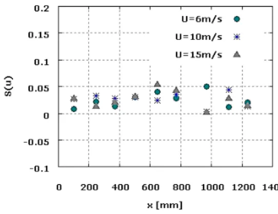
Many of the formulas listed in this article refer to the isotropic and homogeneous turbulence, so it was important to assess what kind of turbulence we have to do with in the experiment. First of all, isotropy of turbulence of the flow behind the grids was investigated. For reference case, skewness factor along the test section of the tunnel in case without the turbulence generator (grid) and without the flat plate was measured. The first measuring point position was 100 mm from the measurement chamber inlet (230 mm from the upper wall, i.e. in the middle of the chamber). Values of skewness for mean flow velocities U = 6, 10, 15 m/s are displayed in Fig. 6. The turbulence intensity Tu didn’t exceed, in this case, the value of 0.13 %. As one can see, S(u) for all three flow velocities ranges approximately from 0 to 0.06 throughout the measured region.
Fig. 6. Skewness along the measurement chamber in case of no turbulence generator, for
mean flow velocities U = 6, 10 and 15 m/s.
According to the previous investigations (Grzelak, Wiercinski, 2015), turbulence of the flow behind grids was considered to be nearly isotropic from the distance x/M≈ 60. The values of x/M, S(u), K(u) for grids G1 – G4 and for all flow velocities used in the experiment are displayed in Table 1. (For G1 the distance is x/M = 90, but it was the first point measured behind the grid, i.e. x = 90 mm).
Table 1 Values of the distance x/M for grids G1 –
G4, from which turbulence is considered to be isotropic
Grid U / S(u) K(u) X/M
G1
10 0.050 3.00 90
15 0.057 3.00 90
20 -0.033 3.03 90 G2
10 0.036 2.90 60
15 0.036 2.90 60
20 0.057 2.88 70
G3
6 0.049 2.93 60
10 0.059 2.94 66
15 0.028 2.94 56
20 -0.024 2.97 66
G4 6 0.047 2.91 61
10 0.060 2.94 67
The homogeneity of turbulence behind all grids used in the experiment was investigated. As a method to investigate the homogeneity of the flow behind the grid, one can use transverse variation of the difference of the root mean square of the downstream velocity,
2 1 2
u
, and the centreline value normalized by the centreline value, 2120 u (Mohamed and LaRue 1990):
122 0
2 1 2 0 2 1 2
u
u
u
u
V
(15)Finally, it can be stated that turbulence of the flow over the plate is nearly isotropic and homogeneous for grids G1 – G4 (grid G5 produced anisotropic, inhomogeneous flow, which was due to the fact that the mesh of G5 was too large to allow the exploration of regions with sufficiently large values of x/M where homogeneity could be expected to be recovered).
5.3
Scales of Turbulence
To investigate the turbulence scale dependence on the transition inception, which was the main goal of the experiment, determining the length scale behind the grid was first needed. To determine the dissipation scale Lu and Kolmogorov scale , knowledge of the rate of turbulence kinetic energy dissipation was required. Therefore the turbulence energy spectrum E(k) was determined by means of Fourier transform in Matlab.
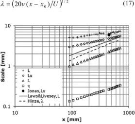
In Fig. 9 different kinds of turbulence length scales are presented, for the selected grid G3, the velocity of the flow U = 10 m/s and the grid distance Ls= 450 mm from the leading edge of the plate. The integral scale L, associated with the largest eddies in the flow has of course the largest dimension, next we have a bit smaller dissipation scale Lu, Taylor microscale λ and finally the Kolmogorov scale as the measure of the smallest eddies. The results of Jonas (2000), for dissipation scale Lu, was provided for comparison. The solid line in Fig. 9 corresponds to the typical variation of the integral scale (see Laws and Livesey 1978):
1/20)
(x x M A
L L , M / d5 (16)
Where AL= 2 or AL= 0.1 (Kurian and Fransson 2009); x0 is a virtual origin of turbulence. For the present grid G3: M/d = 2.5 and x0 = 8.7 mm. The dashed line in Fig. 7 corresponds to the variation of the Taylor microscale given by Hinze (1975):
1/20)
(
20 xx U
(17)Fig. 7. Scales of turbulence behind the grid G3,
for U = 10 m/s; + L – integral scale (2), Lu –
dissipation scale (7), λ – Taylor microscale (9),
□η – Kolmogorov scale (11).
5.4
Velocity Profiles in the Boundary Layer
Next, the velocity profiles in the boundary layer on a flat plate were measured. Distance between the
measuring points in the x direction was 20 mm. The origin of the x-axis was the leading edge. In each of the points the boundary layer profile was measured. Each profile consisted of about 40 points; the first one at 25 mm and the last one about 0.1 mm above the plate surface. The distance from the hot-wire to the plate, Y0, was measured by means of the method called ‘hydraulic zero’ (Epik 1998). If the wire was very close to the surface, thermo anemometric response was like velocity started to increase. Then the measurements were stopped. For the further procedure it was assumed that the last measured point was Y = 0 mm from the wall. To find a real Y0, the velocity profile U = f(Y) was examined (Fig. 8). Because U|wall= 0, a tangent to the profile, U = (dU/dY)Y+B, was conducted through the last few points of the profile (points for which the velocity seemed to increase, were rejected). The intersection of the tangent and the abscissa gives, as the absolute value |Y0|, the searched distance from the hot-wire to the plate surface.
Fig. 8. Velocity profile in a boundary layer, for
G3, U = 10 m/s, LS = 450 mm.
The measured boundary layer thickness, defined as U ( ) = 0.99 U∞, was from about 1.3 to 3 mm for laminar boundary layer and from about 9 to 14 mm for turbulent boundary layer. The examples of the boundary profiles, for grid G3, U = 10 m/s, LS = 450 mm, are presented in Figs. 9 and 10, in comparison with other well-known profiles: the Blasius profile for laminar boundary layer (Fig. 9) and the law of the wall for turbulent boundary layer (Fig. 10). In both cases, three different distances, x, from the leading edge are taking into account. First one is x = 110 mm, where the boundary layer is still laminar (shape factor H = δ*/δ** = 2.25). Next profile, for x = 370 mm, lays in the transition region (H=1.91; the onset of transition is estimated to xt = 313 mm). The last profile, x = 650 mm, corresponds to the turbulent boundary layer (H = 1.42).
To avoid separation at the leading edge the incidence angle of the plate i = –1.63° was set (boundary layer with favourable pressure gradient). Therefore a velocity gradient along the plate was measured. A value of the acceleration parameter:
dx dU U
a
2 (18)kinematic viscosity, was approximately equal to a ≈ 2.7·10-7. This showed that compared with the critical acceleration parameter needed to accomplish relaminarizationin boundary layers (acrit 3.5×10⁻⁶, see e.g. Sreenivasan1982), the applied pressure gradient is quite moderate. In terms of velocity increase it is from about 2 to 4%.The effect of favourable pressure gradient on boundary layer receptivity and on turbulence characteristics one can find e.g. in Xu et al. (2016), Johnson and Pinarbasi (2014), Kurian and Fransson (2009). According to the experiment of the last authors, who reached the acceleration parameter maximally equal to 2.5·10-7, an important result is the observed reduction in turbulence length scales (20-30%) for large mesh widths (M = 36 mm), which was absent for small mesh widths (M = 4.2 mm).
Fig. 9. Blasius profile for the laminar boundary
layer; boundary profiles for G3, U = 10 m/s and
three distances x from the leading edge.
Fig. 10. The law of the wall for turbulent boundary layer; boundary profiles for G3,
U = 10 m/s and three distances x from the
leading edge.
5.5
Method of Determining the
Transition Inception
Having determined the length scale of turbulence, the momentum thickness Reynolds number of the onset of the transition, Ret**, needs to be calculated, to find the correlation function. The values of the local skin friction coefficient, Cf, were used to observe the region of transition and to determine the intermittency factor by means of Eq. (19), derived
from the model of Dhawan and Narasimha (1958).
fl fl
fl f
C C
C C
(19)Cfl and Cft are local skin friction coefficients in laminar and turbulent regions of the flow, respectively. They were determined by means of the Blasius solution for the laminar and turbulent boundary layer (Blasius 1913): Cfl=0.664(Rex)-0.5, Cft=0.0595(Rex)-0.2. The intermittency factor was first defined by Townsend (1948) as the fractional time spent by a fixed probe in the turbulent fluid. Next, another formula for intermittency factor, γ (20), was used to set the characteristics of the laminar-turbulent transition. To describe γ in the transition region the cumulative distribution function of three-parametric Weibull probability distribution was used (Dhawan and Narasimha 1958, Emmons 1951):
* * * *
* * * *
Re Re
Re Re exp 1
t
t (20)
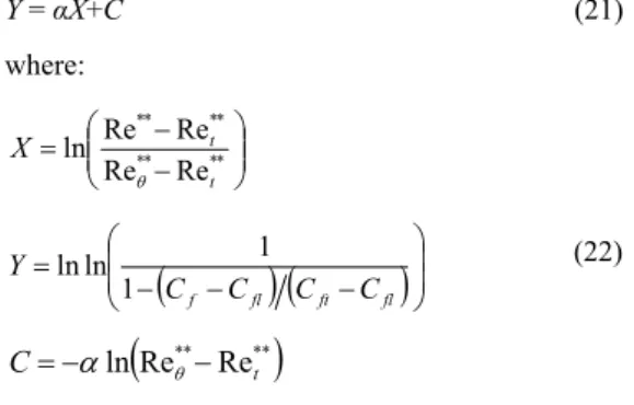
The description of the Weibull distribution and its application in different engineering fields can be found in Lipson and Sheth (1973) or Wadsworth (1989). In the Eq. (20) α is the shape parameter, Ret** – the point where transition begins, Re** – (characteristic length) the point where intermittency factor is equal to (e − 1)/e = 0.632, where e is a base of the natural logarithm. Taking twice the logarithm of Eq. (20) and substituting Eq. (19) for γ,it is possible to determine the Ret** obtaining the linear relationship (Lipson and Sheth 1973):
Y = αX+C (21) where:
** **
* * * *
Re Re
Re Re ln
t t
X
fl ft fl
f C C C
C Y
1
1 ln
ln
(22)
Re** Re**
ln t
C
A shape parameter α is a slope of the function Y = αX+C. This method was validated for the experimental data presented in the paper of Wiercinki (1997).
Fig. 11. Intermittency factor, determined from
the Eq. (19), in the function of Re**.
Fig. 12. Function (21).
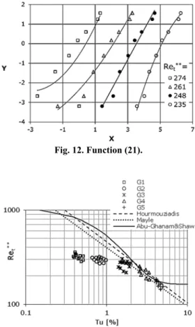
Fig. 13. Momentum thickness Reynolds number at the onset of transition as a function of turbulence intensity for different grids, flow velocities and grid distances; lines represent
formulas (23), (24) and (25).
5.6
Correlations of the Transition
The freestream turbulence intensity at the leading edge for grids G1 – G4 was from Tu = 0.4 % to 3.4 % and for grid G5 exceeded the value of 4 %, moreover the turbulence was not isotropic at the measured points in case of grid G5. Fig. 13 shows dependence between the turbulence intensity at the plate leading edge, Tu, and the momentum thickness Reynolds number of the onset of transition, Ret**, in comparison with some known correlations: Hourmouziadis (1989):
65 . 0 *
*
460
Ret Tu (23) Mayle (1991):
8 / 5 *
* 400
Ret Tu (24) And Abu-Ghannam and Shaw (1980):
Tu
t 163exp6.91
Re** (25) One can see, that for Tu< 2 % (it refers to grids G1, G2 and partly G3) the transition inception appears earlier than it follows from the mentioned correlations.
To create the first correlation with turbulence length scale, the dissipation scale Lu values at the leading edge of the plate were used. The results of present investigations seem to confirm the results of Jonas (2000), but only if we make correlation for all grids together (Fig. 14a; dashed line represents the Eq. (1)). But when we look at every grid separately, the result seems not to be that obvious. Because of the result points dispersion the investigations need to be verified, but according to the present ones the momentum thickness Reynolds number Ret** increases (which means the transition appears later) when Lu increases, for grids G2 and G3. If the values of the Reynolds number Ret** start to become smaller than 200 (as we have for the grid G5), the transition appears earlier when the values of the length scale Lu are larger.
The turbulence scale at the Eq. (1) can be changed in the non – dimensional formula using one of the grid parameters. Wire diameter, d, has been chosen:
m t
d Lu
k
* * Re
(26)
Figure 14b shows the results for Ret** as a function of Lu/d, for grids of different dimensions. For G1 – G4: coefficient of the Eq. (26) is k = 158, exponent m = 0.455. When the value of Lu/d increases, the transition appears later for the grids G1 – G4 and earlier for the grid G5, but we keep in mind that in the last case the turbulence is anisotropic. Besides, the values for the grid G4 seem to belong to both correlations. It is interesting to note that the minimum value of transition Reynolds number presented in Figs. 14a and 14b is in a good agreement with the classical solution obtained from the theory of hydrodynamic stability: Ret** = 161. Because in case of the grid G5 turbulence was neither isotropic nor homogeneous at the measured points over the plate, it seems reasonable to neglect the results for this grid in the following part of the article.
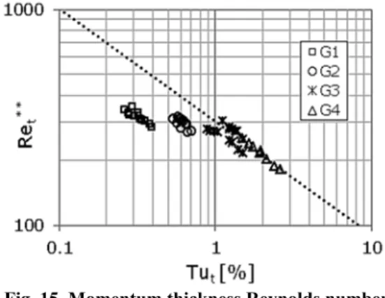
find any good correlation function for Tut and Ret. The next Fig. 16 displays Ret** as a function of the dissipation length scale Lut at the onset of transition. For small levels of free stream turbulence, i.e. Tut< 1.5 % (which was obtained for grids G1, G2 and almost for all used velocities and grid distance Ls in case of G3 (U = 6, 10 m/s for all grid distances and U = 15 m/s for Ls = 450, 410, 370 mm), the dissipation scale increases with the decreasing of Ret**. For the further increasing of the level of turbulence, i.e. for G3 (U = 15 m/s, Ls = 330 mm and U = 20 m/s, Ls = 370, 330 mm) and for G4 (U = 6 and 10 m/s, all grid distances) the influence of the turbulence scale on the beginning of transition isn’t significant. Fig. 17 displays the relation between turbulence scale and intensity at the onset of transition. With the increasing of Tut, Lut also increases, but only to the level of turbulence Tut≈ 1.5 %, then Lut slowly starts to reach a constant value.
(a)
(b)
Fig. 14. Momentum thickness Reynolds number
at the onset of transition as a function of Lu,
(Fig.14a) and Lu /d (Fig.14b) for different grids,
flow velocities and grid distances; dashed line in Fig.14a represents the Eq. (1).
The correlation Ret** = f (Lut) can be made non – dimensional by means of the momentum thickness of the boundary layer, **:
mt t
t
k
Lu
* * *
*
/
Re
(27) Figure 18 presents Ret** as a function of Lutdivided by the momentum thickness at the onset of transition, t** ( t** was found from the formula
Ret** = U t**/ ν, where U – streamwise velocity, ν –
kinematic viscosity). One can observe a similar trend as for previous correlation (Fig. 16). For small
levels of turbulence, Tut< 1.5 % (G1, G2, G3),
dissipation scale divided by t** increases with
slight decreasing of Ret**. For Tut> 1.5 % (G4 and
G3: U = 15 m/s, Ls = 330 mm and U = 20 m/s, Ls =
370, 330 mm) further decreasing of Ret**seems not
to depend on changes in the ratio Lut/ t**, which
tends to the constant value.
Fig. 15. Momentum thickness Reynolds number at the onset of transition as a function of
turbulence intensity Tut, at the onset of
transition, for different grids, mean flow velocities and grid distances.
Fig. 16. Momentum thickness Reynolds number
as a function of turbulence scale Lut, at the onset
of transition, for different grids, mean flow velocities and grid distances.
Fig. 17. Dissipation length scale Lut as a function
of turbulence intensity Tut, at the onset of
Fig. 18. Momentum thickness Reynolds number
as a function of the ratio Lut/δt**at the onset of
transition, for different grids, mean flow velocities and grid distances.
Fig. 19. Momentum thickness Reynolds number as a function of the Taylor Reynolds number
at the onset of transition, for different grids, mean flow velocities and grid distances.
Fig. 20. Momentum thickness Reynolds number
as a function of turbulence intensity, Tut,
and ratio Lut/δt**at the onset of transition.
The next correlation is related with another turbulence length scale: Taylor microscale λ. The information about λ is sufficient to parameterize by-pass transition with free-stream turbulence intensity and scale, since it leads over dissipation rate
2 2
/
15
u
(where u’ is the streamwise velocity standard deviation) and turbulent kinetic energy to other scales and permits to link, over the transport equations, with the turbulent stresses. Fig.19 displays the onset Reynolds number Ret**as a function of Taylor Reynolds number
t u
Re at the onset of transition. This time all data presented in Fig. 19 (for grids G1 – G4) are divided into two ranges: for Tut
0.26;1.5
%and,
1
.
5
;
2
.
6
%
t
Tu
which correspond to values of the turbulence level at the leading edge:
0
.
4
;
2
%
t
Tu
,Tu
t
2
;
3
.
4
%
, respectively. Asprevious, the first range concerns with grids G1, G2 and G3 (U = 6, 10 m/s for all grid distances and U = 15 for Ls= 450, 410, 370 mm), the second range
concerns with grid G3 (U = 15 m/s, Ls = 330 mm
and U = 20 m/s, Ls = 370, 330 mm) and G4 (U = 6
and 10 m/s, all grid distances). When Tut< 1.5 %
the onset of transition approaches the plate leading edge with the increasing of Reλt. After exceeding
the level of 1.5%, the onset Taylor Reynolds number starts to tend to the constant value.
Finally, two last Figs. (20, 21) present simultaneous impact of turbulence intensity and turbulence scale on the boundary layer transition. Taking into account the turbulence intensity, Tut, at the onset of
transition and the turbulence scale, Lut, divided by
the momentum thickness at the onset of transition,
t**, we can write the Eq. (28), which is – to some
extent – generalization of the correlation given by the Eq. (27).
Fig. 21. Momentum thickness Reynolds number
as a function of turbulence intensity, Tut,
and Taylor Reynolds number, Reλt, at the onset
of transition.
2
1
* * *
*
Re
m
t t m t t
Lu
kTu
(28)
Taking logarithm of the above formula, we get an equation of a plane:
* * 2 1
*
* log log log
Re log
t t t
t
Lu m Tu m k
(29)
which is displayed in Fig. 20.The searched constants at the above formula were found by means of the three-dimensional regression procedure: k = 271, m1 = – 0.206, m2 = – 0.015.
Analogously, a correlation related to the Taylor Reynolds number at the onset of transition can be written:
2
1
Re
The Eq. (30) is displayed in Fig. 21 and the searched constants are: k = 201, m1 = – 0.287, m2 = 0.088. Looking at above two formulas (28), (29) and the exponentsm1, m2 it can be stated that turbulence intensity is the primary factor affecting transition while turbulence length scale has only a secondary affect.
6. C
ONCLUSIONTo investigate the phenomena of turbulent flow, five wicker grids with square meshes and different parameters were used to generate turbulence. The turbulence intensity at the leading edge of the plate was from Tu = 0.4 % to 4 %. Several longitudinal scales of turbulence were determined, i.e. integral scale L, dissipation scale Lu, Taylor microscale λ and Kolmogorov scale . To assess the isotropy of turbulence, the skewness factor of the flow velocity distribution was determined. For grids G1 to G4, i.e. for (d = 0.3 mm, M = 1 mm, Tu = 0.4 %) to (d = 3 mm, M = 10 mm, Tu = 3.4 %) the isotropic homogeneous turbulence throughout the measured chamber was obtained.
The influence of the turbulence scale on the laminar–turbulent bypass transition location on a flat plate was investigated. In this case the dissipation scale Lu at the leading edge was taken into account. For this purpose, the momentum thickness Reynolds number Ret**, at which transition onset appears, was calculated. Present investigations seem to confirm the results indicating that the boundary layer laminar–turbulent inception moves downstream with the decreasing of turbulence scale, but only if we make correlation for all grids together. When we take into account a single grid, especially G2 (d = 0.6 mm, M = 3 mm) and G3 (d = 1.6 mm, M = 4 mm), the results are not so obvious or even seem to be quite opposite. Dividing the turbulence scale by the grid wire diameter, non–dimensional formula was developed (26). The investigation indicates that the reducing of turbulence scale (divided by the grid wire diameter d) provides an earlier inception, i.e. the lower momentum thickness Reynolds number for grids G1 – G4.
The next presented correlations, refer to free stream turbulence intensity, Tut, and free stream turbulence dissipation length scale, Lut, at the onset of transition. It was observed that for small levels of free stream turbulence (Tut< 1.5 %) the dissipation scale Lut increases with the decreasing of Ret**. For Tut> 1.5 %, the influence of the turbulence scale on the beginning of transition isn’t significant. Similar conclusion was obtained for Lut divided by the momentum thickness at the onset of transition, t** (27). For Tut< 1.5 % the ratio Lut/ t** increases with slight decreasing of Ret**; for higher level of turbulence, Lut/ t** tends to the constant value. The onset Reynolds number Ret** as a function of Taylor Reynolds number Reλ= u’λ /ν (where λ is Taylor microscale) at the onset of transition was presented. It was observed that for the intensity range Tut
0.26;1.5
%, which corresponds tovalues of the turbulence level at the leading edge,
0.4;2
%,
Tu the onset of transition approaches the plate leading edge with the increasing of Reλt. ForTut
1.5;2.6
%Tu
2;3.4
%at the leading edge) the onset Taylor Reynolds number starts to tend to the constant value.Finally, simultaneous impact of turbulence intensity and turbulence scale at the onset of transition on the boundary layer transition inception was presented (Figs. 20, 21), showing that turbulence intensity is the primary factor affecting transition and turbulence length scale has a secondary affect.
R
EFERENCESAbu-Ghannam, B. J. and R. Shaw (1980).Natural transition of boundary layers – the effects of turbulence, pressuer gradient, and flow history. J. Mech. Eng. Sci. 22, 213-228.
Ames, F. E. and R. J. Moffat (1990). Heat transfer with high intensity, large scale turbulence: the flat plate turbulent boundary layer and the cylindrical stagnation point. Report No. HMT-44, Department of Mechanical Engineering, Stanford University, Stanford, CA.
Baines, W. D. and E. G. Peterson (1951). An investigation of flow through screens. ASME J. Fluids Eng.73, 467-480.
Barret, M. J. and D. K. Hollingsworth (2001). On the calculation of length scales for turbulent heat transfer correlation. ASME J. Heat Transfer 123, 878-883.
Batchelor, G. K. (1953).The Theory of Homogeneous Turbulence, Cambridge University Press, Cambridge, UK
Birouk, M., B. Sarh and I. Gokalp (2003). An attempt to realize experimental isotropic turbulence at low reynoldsnumber. Flow Turbul. Combust. 70, 325–348.
Blasius, P. R. H. (1913). Blasius, H. (1913). The law of similarity of frictional processes in fluids. (Originally in German), Forsch Arbeit Ingenieur-Wesen, Berlin 131. 1–41.
Dhawan, S. and R. Narasimha (1958). Some properties of boundary layer flow during the transition from laminar to turbulent motion. J. Fluid Mech. 3(04), 418-436.
Emmons, H. W. (1951). The laminar-turbulent transition in a boundary layer, Part I. J. Aeron. Sci. 18, 490-498.
Epik, E. J., E. P. Dyban, V. N. Klimenko, T. T. Suprun and L. E. Jushina (1998). Experimental study of by-pass transition heat transfer, Final report, Kiev.
Fouladi, F., P. Henshaw and D. S. K. Ting (2015). Turbulent Flow Over a Flat Plate Downstream of a Finite Height Perforated Plate. ASME J. Fluid Eng. 137, 021203-1.
turbulence behind a uniform jet grid.J. Fluid Mech. 62, 115-143.
Grzelak, J. and Z. Wiercinski (2015). The decay power law in turbulence generated by grids. Transactions IFFM 130, 93-107.
Hall, D. J. and J. C. Gibbings (1972). Influence of stream turbulence and pressure gradient on boundary – layer transition. J. Mech. Eng. Sci. 14, 134-146.
Hinze, I. O. (1975). Turbulence. McGraw – Hill Book Company.
Hourmouziadis, J. (1989). Aerodynamic Design of Low Pressure Turbines. AGARD Lecture Series 167.
Jimenez, J. (1998). Turbulent velocity fluctuations need to be Gaussian.J. Fluid Mech., 376, 139-147.
Johnson, M. W. and A. Pinarbasi (2014). The Effect of Pressure Gradient on Boundary Layer Receptivity. Flow Turb. Combust. 93, 1-24. Jonas, P., O. Mazur and V. Uruba (2000). On the
receptivity of the by – pass transition to the length scale of the outer stream turbulence. Eur. J. Mech. B-Fluids19, 707-722.
Kurian, T. and J. H. M. Fransson (2009). Grid-generated turbulence revisited. Fluid Dynamics Research 41(2).
Laws, E. M. and J. L. Livesey (1978). Flow through screens.Ann. Rev. Fluid Mech. 10,247-266. Lipson, C. and N. J. Sheth (1973). Statistical design
and analysis of engineering experiments. McGraw-Hill, New York.
Makita, H. (1991). Realization of a large-scale turbulence field in a small wind tunnel. Fluid Dynamics Research 8, 53-64.
Mayle, R. E. (1991). The Role of Laminar – Turbulent Transition in Gas Turbine Engines. Journal of Turbomachinery 113, 509-537. Mohamed, M. S. and J. C. LaRue (1990). The
decay power law in grid-generated turbulence. J. Fluid Mech. 219, 195-214.
Morkovin, M. V. (1969). On the many faces of transition, In Viscous Drag Reduction, ed. CS
Wells, New York: Plenum, 1–31.
Mydlarski, L. and Z. Warhaft (1996). On the onset of high-Reynolds-number grid-generated wind tunnel turbulence.J. Fluid. Mech.320, 331-368. Mydlarski, L. and Z. Warhaft (1998). Passive scalar
statistics in high-Peclet-number grid turbulence.J. Fluid. Mech. 358,135-175.
Noro, S., Y. Suzuki, M. Shigeta, S. Izawa and Y. Fukunishi (2013).Boundary layer receptivity to localized disturbances infreestream caused by a vortex ring collision. Journal of Applied Fluid Mechanics 6 (3), 425-433.
Roach, P. E.(1986). The generation of nearly isotropic turbulence by means of grids.J. Heat and Fluid Flow 8 (2), 82–92.
Shahinfar, S. and J. H. M. Fransson (2011). Effect of free-stream turbulence characteristics on boundary layer transition.J. Physics: Conference Series 318(3).
Sreenivasan, K. R. (1982).Laminarescent, relaminarizing and retransitional flows.Acta Mech. 44, 1-48.
Ting, D. S. K. (2013). Some Basics of Engineering Flow Turbulence. Revised ed., Naomi Ting’s Book, Windsor, Canada.
Townsend, A. A. (1948). Local isotropy in the turbulent wake of a circular cylinder.Aust. J. Sci. Res. 1(2), 161-174.
Valente, P. C. and J. C. Vassilicos (2011). The decay of turbulence generated by a class of multiscale grids. J. Fluid Mech. 687, 300-340. Wadsworth, H. M. (1989). Handbook of statistical
methods for engineers and scientists. McGraw-Hill, New York.
Wiercinski, Z. (1997). The stochastic theory of the natural laminar-turbulent transition in the boundary layer. Trans. IFFM, Gdansk102, 89-110.