Derivation and assessment of a mixed layer sub-mesoscale model

(1)

OSD

6, 2157–2192, 2009

Mixed layer sub-mesoscale

model

V. M. Canuto and M. S. Dubovikov

Title Page

Abstract Introduction

Conclusions References

Tables Figures

◭ ◮

Back Close

Full Screen / Esc

Printer-friendly Version

Interactive Discussion Ocean Sci. Discuss., 6, 2157–2192, 2009

www.ocean-sci-discuss.net/6/2157/2009/

Ocean Science Discussions

Papers published inOcean Science Discussionsare under open-access review for the journalOcean Science

Derivation and assessment of a mixed

layer sub-mesoscale model

V. M. Canuto1,2and M. S. Dubovikov1,3

1

NASA, Goddard Institute for Space Studies, New York, NY, 10025, USA 2

Dept. Appl. Math. and Phys. Columbia University, New York, NY, 10027, USA 3

Center for Clim. Systems Res., Columbia University, New York, NY, 10025, USA

Received: 7 August 2009 – Accepted: 5 September 2009 – Published: 17 September 2009

Correspondence to: V. M. Canuto (vcanuto@giss.nasa.gov)

(2)

OSD

6, 2157–2192, 2009

model

Title Page

Tables Figures

◭ ◮

Back Close

Full Screen / Esc

Interactive Discussion

Abstract

Present studies of mixed layer sub-mesoscales rely primarily on high resolution numer-ical simulations. Only few of these studies have attempted to parameterize the ensuing buoyancy submesoscale fluxes in terms of the resolved fields so that they can be used in OGCMs (ocean circulation models) that do not resolve sub-mesoscales. In reality,

5

OGCMs used in climate studies include a carbon-cycle which also requires the flux of a passive tracer.

The goal of this work is to derive and assess a parameterization of the submesoscale vertical flux of an arbitrary tracer in terms of the resolved fields. The parameterization is obtained by first solving the dynamic equations governing the velocity and tracer fields

10

that describe sub-mesoscales and then constructing second-order moments such as the tracer fluxes. A key ingredient of the present approach is the modeling of the non-linear terms that enter the dynamic equations of the velocity and tracer fields, a problem that we discuss in two Appendices.

The derivation of the sub-mesoscale tracer vertical flux is analytical and can be

fol-15

lowed in detail since no additional information is required. The external forcing includes both baroclinic instabilities and wind stresses.

We compare the model results with data from sub-mesoscale resolving simulations available in the literature which are of two kinds, one with no wind (baroclinic instabilities only) and the other with both baroclinic instabilities and wind. In both cases, the model

20

results reproduce the simulation data satisfactorily.

1 Introduction

While mesoscales are characterized by a small Rossby number Ro=_{ζ /f}_≪_{1 (where}_ζ

andf are the relative and planetary vorticities respectively), sub-mesoscales are char-acterized by Ro∼1 and Ri∼Ro−1/2∼O(1), where Ri is the Richardson number (Thomas

25

(3)

OSD

6, 2157–2192, 2009

model

Title Page

Tables Figures

◭ ◮

Back Close

Full Screen / Esc

Interactive Discussion ocean cannot be extrapolated to describe sub-mesoscales and a new one must be

devised.

Most of our knowledge about mixed layer sub-mesoscales comes from high resolu-tion studies carried out by several groups (Levy et al., 2001, 2009; Thomas and Lee, 2005; Mahadevan, 2006; Mahadevan and Tandon, 2006; Klein et al., 2008; Thomas et

5

al., 2008; Capet et al., 2008). These studies have revealed many interesting features of sub-mesoscales especially their contribution to the vertical mixing of mass, buoyancy and tracers in the upper ocean. Among the most salient eff_{ects of sub-mesoscales}

on global ocean properties is the well documented tendency to re-stratify the mixed layer (Spall, 1995; Nurser and Zhang, 2000). The eff_{ect of sub-mesoscales on deep}

10

convection has been recently demonstrated by Levy et al. (2009, Fig. 9) who point out a better agreement with the new mixed layer data by Boyer Montegut et al. (2004) south of the WBC (Western Boundary Current). Even in non-convective regimes, one can expect a significant cancellation between sub-mesoscale and small scale fluxes leading to the mixed layer re-stratification (e.g., Capet et al., 2008, Fig. 12; Klein et

15

al., 2008, Sect. 4); specifically, Hosegood et al. (2008) estimated that sub-mesoscales contribute up to 40% of the re-stratification process. In addition, as noted by Lapeyre et al. (2006) and Klein et al. (2008), the surface layers re-stratification is compensated by de-stratification of the ocean interior pointing to an interesting dynamical connection between surface and interior processes. Another important eff_{ect of sub-mesoscales}

20

concerns the location of the WBC that is shifted south by 4◦ and whose off_shore

ex-tension penetrates further to the east in better agreement with observations (Levy et al., 2009). An earlier study by Treguier et al. (2005), which found a significant in-crease (from ∼30 Sv to ∼70 Sv) in the barotropic transport in the Gulf Stream when moving from 1◦ to 1/6◦ resolution, was recently confirmed and the inclusion of

sub-25

mesoscales further increased the transport by ∼50 Sv. Finally, the structure of the MOC (meridional overturning circulation) was also significantly aff_{ected by the}

(4)

OSD

6, 2157–2192, 2009

model

Title Page

Tables Figures

◭ ◮

Back Close

Full Screen / Esc

Interactive Discussion This brief summary of some of the results of very high resolution (1/54◦, ∼2 km)

regional studies is suffi_{cient to highlight the importance of sub-mesoscales and thus}

the question arises as to how much of sub-mesoscale physics is actually accounted for by present day global OGCMs (ocean global circulation models). Even today’s highest resolution global ocean models ∼1/10◦ (Maltrud and McClean, 2005; Sasaki

5

et al., 2008) are not able to capture the sub-mesoscale field and much less are in the position to do so the OGCMs coupled to an atmospheric model used for climate studies where the resolution is at best 1◦ but generally lower. The significant global processes revealed in going from 1◦resolution (∼100 km) and 1/54◦resolution (∼2 km) are presently absent in such global models especially in climate studies. It therefore

10

seems that a reliable parameterization of submesoscales in terms of the resolved fields has become necessary to ensure the physical completeness of mixed layer mixing processes.

When solving the dynamic equations of a coarse resolution OGCM, two key equa-tions are those forT andS (temperature and salinity) but since climate models must

15

also include a carbon cycle, one must consider a general tracer field whose dynamic equation is given by1:

D_tτ+_∇_H _·F_H +_∂_z_F_v

| {z }

mesoscales

+_∇_H _·F_H +_∂_z_F_v

| {z }

sub−mesoscales

=_∂_z₍_K_v_∂_z_τ₎+_Q_ext _(1a)

where for completeness we have included the contribution of mesoscales which are however not treated in this work which is restricted to mesoscales. The

sub-20

mesoscales horizontal and vertical fluxes are defined as follows:

F_H(τ)≡u′_τ′_, _F

V(τ)≡w′τ′ (1b)

1_D

(5)

OSD

6, 2157–2192, 2009

model

Title Page

Tables Figures

◭ ◮

Back Close

Full Screen / Esc

Interactive Discussion where a prime denotes the submesoscale fields and an overbar stands for an

en-semble average over resolved scales. However, since the horizontal sub-mesoscales flux is smaller than the corresponding one due to mesoscales, we shall concentrate on the parameterization of the vertical sub-mesoscale flux, F_V(τ). The methodology we employ to carry out the parameterization contains three steps: first, one solves

5

in Fourier space the sub-mesoscale dynamic equations describing the sub-mesoscale fieldsw′, τ′; second, one forms the averages of the product of the two fields so as to obtain the second-order correlationw′_τ′ _{and third, one integrates over all} wavenum-bers to obtain the final expression forF_v in coordinate space and expressed in terms of the resolved fields, to be used in Eq. (1a). The procedure was first worked out for the

10

linear case by Eady and later by Killworth (1997) and for the non-linear case by Canuto and Dubovikov (2005, 2006, CD5,6). Though the dynamic equations describing the velocity and temperature fields are formally the same as those describing mesoscales that were discussed in CD5–6, in the present case they must be solved in the regime appropriate to sub-mesoscales represented by Ro=_{ζ /f}=_O_{(1) rather than Ro}_≪_{1 as in}

15

the case of mesoscales which leads to the appearance of terms that were not present in the Ro≪1 regime.

The key diffi_{culty in solving the sub-mesoscale dynamic equations is represented by}

the non-linear terms whose closure is expressed in Eq. (3a) below. Since the latter is a key ingredient of the present model and since the original derivation (Canuto and

20

Dubovikov, 1997) is rather involved, in Appendices A, B we have attempted to find a way to present a more physical approach to Eq. (3a) with the goal of highlighting the physical rather than the technical features of Eq. (3a).

In addition to the derivation of the closure relations (Eq. 3a), there is the issue of the assessment of Eq. (3a) when applied to flows diff_{erent than the present one so}

25

(6)

nec-OSD

6, 2157–2192, 2009

model

Title Page

Tables Figures

◭ ◮

Back Close

Full Screen / Esc

Interactive Discussion essary but not sufficient for the credibility of the parameterization of sub-mesoscale

fluxes we derive in Sects. 5–6. The additional requirement consists in assessing the model predictions against results from sub-mesoscale resolving simulations of the type cited in the first part of this discussion. The first simulation corresponds to a system forced by baroclinic instabilities and no wind (Fox-Kemper et al., 2008, FFH, 2 km

reso-5

lution) and the second one consists of a flow under realistic wind and buoyancy forcing (Capet et al., 2008, 0.75 km resolution). We shall present a detailed comparison of our parameterization with these simulation data.

To make the sub-mesoscale model results usable in OGCMs, we looked for analyt-ical solutions of the sub-mesoscale dynamic equations and to achieve that goal, we

10

introduced one approximation that consists in assuming that the fluxes are mostly con-tributed by their spectra in the vicinity of their maxima. Though this introduces errors of several tens of a percent, the advantages of obtaining analytic expressions for the vertical tracer flux in terms of resolved fields in the presence of both frontogenesis and Ekman pumping and for an arbitrary Ri, was worth exploring. Following Killworth

15

(2005) suggestion, we adopt the approximation that due the mixed layer strong mixing, one can neglectτz. Anticipating our main result, the vertical gradient of the vertical flux

that enters in the original Eq. (1a) will be shown to have the following form:

∂zFV(τ)=u

+

S · ∇Hτ (1c)

whereu+_S plays the role of a bolus velocity. Sinceτ_zis small, one may make the analogy

20

with the mesoscale bolus velocity more complete by adding to Eq. (1c) the termw_S+τ_z, wherew_S+ is found from the continuity condition ∂zw

+

S+∇H·u

+

S = 0 (Killworth, 2005).

From Eq. (1c) we shall derive the vertical flux which we write as:

F_V(τ)≡w′_τ′₌₋_κ

H · ∇Hτ, κH =κH(∇hb, u=ug+ua) (1d)

whereu_g,aare the geostrophic and a-geostrophic velocity components, the latter being

25

a key component in the case of strong winds.

(7)

OSD

6, 2157–2192, 2009

model

Title Page

Tables Figures

◭ ◮

Back Close

Full Screen / Esc

Interactive Discussion the turbulence closure model to the non-linear term in the sub-mesoscale tracer

equa-tion in Fourier space in the vicinity of the maximum of the energy spectrum and find the solutions for the tracer fieldτ′; in Sect. 4 we do the same with the sub-mesoscale for the momentum equation and derive an expression for the submesoscale fieldu′. Using these results, in Sect. 5 we compute the spectrum of∂zFV in the vicinity of its

maxi-5

mum and then compute∂zFV and Fv in physical space in terms of resolved fields as

well as the sub-mesoscale eddy kinetic energyK_E. In Sect. 6 we expressK_Ein terms of the resolved fields that, together with the results of the previous section, complete the problem of expressing∂zFV in the presence of both frontogenesis and Ekman

pump-ing. In Sect. 7 we study the case of a strong wind when the Ekman velocity exceeds

10

the geostrophic one. We shall show that when a strong wind blows in the direction of the geostrophic wind or of∇Hb, it tends to de-stratify the mixed layer but at the same

time it generates sub-mesoscales that have the tendency to re-stratify the mixed layer. In both cases, “Ekman flow advects denser water over light” (Thomas et al., 2008). On the other hand, when the wind blows in opposite directions to the previous ones, it

15

tends to re-stratify the mixed layer and does not generates submesoscale eddies. In Sect. 8 we compare the model results with the data from the sub-mesoscale resolving simulations of Capet et al. (2008). In Sect. 9 we compare the model results for the no-wind case with the FFH simulation data. In Sect. 10, we present some conclusions.

2 Sub-mesoscales dynamic equations near the surface

20

Consider an arbitrary tracer fieldτ. Separating it into a mean and a fluctuating part,

τ=_τ+_τ′_{, the dynamical equations for the sub-mesoscale tracer field}_τ′ _{are obtained by}

subtracting the equation for the mean tracerτ from that of the total field. Since this procedure is well known and entails only algebraic steps and no physical assumptions, we cite only the final result (for the notation, see the footnote):

25

D_tτ′=₋U′_{· ∇}_τ₋_Qτ

H−Q τ

(8)

OSD

6, 2157–2192, 2009

model

Title Page

Tables Figures

◭ ◮

Back Close

Full Screen / Esc

Qτ_H ≡u′_{· ∇}

Hτ′−u′· ∇Hτ′, Q_Vτ ≡w′τ′z−w′τ′z (2a)

where the function Q’s represent the non-linear terms; ∇H is the horizontal gradient

operator, an overbar stands for an ensemble average over resolved scales and the ver-tical diff_usivity_K_v _{represents small scale mixing processes. As expected, the average}

of Eq. (2a) yields identically zero. It must be noted that in Eq. (2a) no closure has

5

been used for the sub-mesoscale fields. Equation (2a) formally coincides with those describing mixed layer mesoscales tracer fields studied by Killworth (2005). The dif-ference in representing mesoscales and sub-mesoscales lies in the scales over which the averages (represented by an overbar in Eq. 2a), is taken: in the mesoscale de-scription, averages are over scales exceeding mesoscales while in the description of

10

submesoscales, averages are meant to be over scales smaller than mesoscales but larger than submesoscales. Furthermore, in describing mesoscales one has Ro≪1 and Ri≫1, whereas in the case of submesoscales Ro, Ri∼O(1). Following Killworth (2005), we neglect the terms containingτzandτ′z. Then, the first of Eq. (2a) simplifies

to:

15

∂_tτ′+u¯ · ∇Hτ′=−u′· ∇Hτ−Q_Hτ (2b)

Without the non-linear term, this equation is equivalent to Eq. (2) of Killworth (2005) for the mesoscale buoyancy field in the mixed layer. Within the same approximation, the equation for the horizontal eddy velocity is given by:

∂tu′+u¯· ∇Hu′=−ρ−1∇Hp′−u′· ∇Hu−fez×u′−Q_Hu (2c)

20

Qu_H ≡u′_{· ∇}

Hu′−u′· ∇Hu′ (2d)

wheree_z is the unit vector along z axis. Next, we Fourier transform Eq. (2b,c) in hor-izontal planes and time. Following Killworth (1997, 2005), we keep the same notation

u′_{, τ}′_{for the submesoscale fields in the}_k₋_ω_{space and assume that the mean fields} uand∇Hτare constant in time and horizontal coordinates when Eq. (2b,c) are Fourier

(9)

OSD

6, 2157–2192, 2009

model

Title Page

Tables Figures

◭ ◮

Back Close

Full Screen / Esc

Interactive Discussion transformed. Thus, we obtain:

i(k·u¯−ω)τ′=₋u′_{· ∇}

Hτ−QτH

i(k·u¯−ω)u′₌₋_u′_{· ∇}

Hu−fezxu′−QuH−ikρ−1p′

∂zw′=−∇H ·u′=−ik·u′ (2e)

where we have added the continuity equation that provides the z-derivative of w’. We

5

recall thatτ′, u′ and the non-linear terms are functions of the horizontal wave vector and frequency (k,ω) and z while u¯ is a function ofz only and∇Hτ is z independent.

The solution of Eq. (2e) provides the necessary ingredients to construct the vertical flux (Eq. 1b). On the other hand, since in the dynamical equation (Eq. 1a) we only need

∂_zF_V, we shall write it as follows:

10

∂_zF_V =_w′

zτ′+w′τ′z ≈w′zτ′ (2f)

where in the last expression we have neglected the termw′_τ′

z in accordance with the

adopted approximation and since it is of a higher order inz.

3 The sub-mesoscale tracer fieldτ′

As discussed in Appendices A, B, in the vicinity ofk=_k₀_{corresponding to the maximum}

15

of the eddy energy spectrumE(k), the non-linear termsQ_H have the following forms:

Qτ_H(k, ω)=_{χ τ}′₍_{k, ω}₎_{, Q}u

H(k, ω)=χ u

′₍_{k, ω}₎_{, χ} ₌_k 0K

1/2

E , KE =

1 2|u

′_|2 _(3a)

whereu′ _{is here understood to be in physical space and}_ℓ=_k−1

0 is the characteristic submesoscale length scale. As it is stressed in the literature on this subject (e.g., review by Thomas et al., 2008; Fox-Kemper and Ferrari, 2008; Boccaletti et al., 2007),

20

ℓ is closely related to the deformation radius in the mixed layer, which implies that:

(10)

OSD

6, 2157–2192, 2009

model

Title Page

Tables Figures

◭ ◮

Back Close

Full Screen / Esc

Interactive Discussion wherehis the depth of the mixed layer andNis the buoyancy frequency. Equation (3b)

can also be derived by solving the eigenvalue problem to which the submesoscale equations reduce and which is analogous to the eigenvalue problem in the case of mesoscale (see CD5). Substituting Eq. (3a) into the tracer equation Eq. (2e), we obtain the expression for the submesoscale tracer field:

5

τ′= u ′_{· ∇}

Hτ

χ+ _i₍k·u−ω) (3c)

where |k| = _k₀_{. As in the case of mesoscale discussed in CD5, the frequency} _ω_,

obtained from solving the eigenvalue problem mentioned above, yields the following dispersion relation:

ω(k)=_k_·_u_d _(3d)

10

This relation can be interpreted as the Doppler transformation for the frequency pro-vided that in the system of coordinates moving with the velocityu_d, the submesoscale flow is stationary in which caseω=_{0. Stated in di}ff_{erent words, relation Eq. (3d) implies}

thatu_d is theeddy drift velocity whose expression in terms of mean fields is analogous to that for the case of mesoscales given in Eq. (4f) of CD6:

15

u_d =_h_u_i+ 1

2ℓ 2

e_z× β−fh∂_zLi (3e)

whereL=_−∇_H_b/N2_{is the slope of isopycnal surfaces and}β=_∇_f_{. The bracket}

averag-ing is defined as follows:

h•i ≡

0 Z

−h

(•)K_E1/2(z)d z/

0 Z

−h

K_E1/2(z)d z (3f)

Due to the smallness of the scaleℓ characterizing submesoscales, the second term in

20

Eq. (3e) is negligible and thus:

(11)

OSD

6, 2157–2192, 2009

model

Title Page

Tables Figures

◭ ◮

Back Close

Full Screen / Esc

Interactive Discussion which changes Eq. (3c) to the form:

τ′=₋ u ′_{· ∇}

Hτ

χ +_ik·eu, ue

=_u₋_h_u_i_, _χ = _ℓ−1_K1/2

E (3h)

Relation (Eq. 3d) implies that the dependence of the submesoscale fields on ωis of the form:

A′(ω,k)=_A′₍_k₎_δ₍_ω₋_k_·_u_d₎ _(3i)

5

and therefore in (t,k)-space the fieldsA′depend on time as follows:

A′(t,k)=_A′₍k)exp(−ik·u_dt) (3j) Due to relations Eq. (3i,j), after substituting Eq. (3a) in Eq. (2e), the latter may be solved in both (ω,k) and (t,k) representations.

4 The sub-mesoscale velocity fieldw′

10

It is convenient to begin by splitting the mesoscale velocity field u′ _{into a rotational}

(divergence free, solenoidal) and a divergent (curl free, potential) components:

u′₍_k₎₌_u

R(k)+uD(k); uR(k)=n×ezuR(k), uD(k)=nuD, n=k/k (4a)

and thus the third equation in Eq. (2e) becomes:

∂zw′=−ik·u′=−i kuD (4b)

15

To determineu_R,D, we substitute the second relation (Eq. 3a) in the second equation in Eq. (2e) and derive the following expressions:

u_D =_f−1₍_χ+_ik·ue)u_R, u_R =₋ i kρ

−1_p′

1+_f−2₍_χ+_ik·eu)2, e

(12)

OSD

6, 2157–2192, 2009

model

Title Page

Tables Figures

◭ ◮

Back Close

Full Screen / Esc

Interactive Discussion These relations, as well as Eq. (3h), are valid in both (ω,k) and (t,k) representations.

Below we will use them in the (t,k) representation together with Eq. (3j). To illustrate the physical content of the second of Eq. (4c), we notice that it can also be written, using the third of Eq. (3h), as:

uR =−

i kρ−1p′

1+_Ro2 , Ro = u

′

f ℓ (4d)

5

where Ro is the Rossby number. Thus, in the quasi-geostrophic approximation corre-sponding to small Ro, the first relation in Eq. (4d) reduces to the geostrophic relation

uR→ug=−i kρ−1p′. However, since in the submesoscale regime typically Ro∼1, one

must consider the complete expressions Eq. (4c). That is the reason why we have not calledu_R the geostrophic component andu_Dthe a-geostrophic one.

10

Substituting Eq. (4c) into Eq. (4b), we obtain the expression for∂zw′which allows us

to compute Eq. (2f). NOTE. Readers not interested in the details of the derivation can move directly to the final result Eq. (7a,b).

5 Sub-mesoscale vertical tracer flux

The strategy used to derive submesoscale fluxes, which are bilinear correlation

func-15

tions, consists in computing these functions in (t,k)-space which, in the approximation of homogeneous and stationary mean flow, have the form:

A′₍_t,k′₎_B′∗₍_t,k₎=_A′_B′∗₍_k₎_δ₍_k₋_k′₎ _(4e)

and, because of relation Eq. (3j), relation Eq. (4e) does not depend ont. The function

Re[A′_B′∗₍_k_{)] is usually referred to as the density of}_A′_B′ _in_k_{-space. The spectrum of}

20

the correlation functionA′_B′_is:

A′_B′₍_k₎=

Z

(13)

OSD

6, 2157–2192, 2009

model

Title Page

Tables Figures

◭ ◮

Back Close

Full Screen / Esc

Interactive Discussion i.e., the spectrum ofA′_B′_{is obtained by averaging Re}_A′_B′∗₍_k_{) over the directions of}_k

and multiplying the result byπk. Finally, the correlation functionA′_B′_{in physical space} is obtained by integrating over the spectrum. Following this procedure, from the first of Eq. (3h) and using Eq. (4a,b), we derive the relation:

Rew′

zτ′∗(k)=−Im

n

kχ2_∗(χ +_ik·eu)hu_Du∗_R(k)n_×e_z+_|_u_D_|2₍_k₎_nio_{· ∇}

Hτ (5a)

5

where we have introduced the notation:

χ_∗2≡χ2+₍k·eu)2 (5b)

Next, from the first Eq. (4d) we derive the following relations:

ReuDu∗_R(k)=χ f−1|uR|2(k), ImuDu_R∗(k)=f−1k·ue|uR|2(k) (6a)

|u_D|2₍_k₎₌_χ2

∗f−2|uR|2(k), |u′|2(k)=|uD|2(k)+|uR|2(k)=(1+χ

2

∗f−2)|uR|2(k) (6b)

10

Substituting Eq. (6a) into Eq. (5a) and averaging over the directions ofk, we obtain the spectrum ofw′

zτ′(k). Under the condition

e

K ≤KE (6c)

we obtain:

w′

zτ′(k)=−k02χb

−2h_{χ f}−1_|_u

R|2(k)eu×e+|uD|2(k)eu

i

· ∇Hτ (6d)

15

where:

πk|u_R|2(k)=₍₁+_χ_b2_f−2₎−1_E₍_k_); _πk_|_u_D_|2₍_k₎=₍₁+_χ_b−2_f2₎−1_E₍_k₎ _(6e) E(k)= 1

2πk|u

′_|2₍_k₎_, _χ_b2₌_ℓ−2_{K ,}b _Kb₌_K

E +K ,e Ke =

1 2|ue|

2 _(6f)

E(k) is the spectrum of the total (rotational+_{divergent) eddy kinetic energy. Due to}

relation Eq. (2f), the left hand side of Eq. (6d) multiplied by πk is the spectrum of

(14)

OSD

6, 2157–2192, 2009

model

Title Page

Tables Figures

◭ ◮

Back Close

Full Screen / Esc

Interactive Discussion the z-derivative of the vertical flux ∂_zF_V(k). Thus, multiplying Eq. (6d) by πk, using

Eq. (6e), we obtain the following expression for the spectrum of∂zFV in the vicinity of

the maximum of the energy spectrum:

∂_zF_V(k)=Φ₍_k₎_{· ∇}_H_τ _(6g)

where:

5

Φ₍_k₎=₋_E₍_k₎_k2

0χb

−2h_{χ f}−1₍₁₊_χ_b2_f−2₎−1 e

u×e_z+₍₁+_χ_b−2_f2₎_u_ei _(6h)

With the assumption that the spectraF_V(k) andE(k) have similar shapes, integrating Eq. (6g,h) overk reduces to the substitution of E(k) andFV(k) with the eddy kinetic

energyKE andFV in physical space. The result is:

∂_zF_V(τ)=u+_S · ∇Hτ, u

+

S =−η(eu−λez×ue) (7a)

10

where:

x= KE

e

K , y = ℓf

e

K1/2, η

=_x₍₁+_x+_y2₎−1_, _λ=_yx1/2₍₁+_x₎−1 _(7b)

It is worth noticing that in the second relation in Eq. (7a) the termλe_z×ueis a vector: in fact, althoughe_z×ue is a pseudo-vector (cross product of the vectorse_z andeu),λ∼f is a pseudo-scalar (f is the scalar product of the vectoreand the pseudo-vector 2Ω) and

15

thus the product is a vector.

In Eq. (7a) the velocityu+_S may be interpreted as the sub-mesoscale induced velocity which is a counterpart of the mesoscale induced velocity. As Killworth (2005) noticed, to make the analogy with the mesoscale induced velocity more complete, since in the mixed layer τz is small due to the strong mixing, one may add to Eq. (7a) the term

20

w_S+τ_z, wherew_S+ is found from the continuity condition:

(15)

OSD

6, 2157–2192, 2009

model

Title Page

Tables Figures

◭ ◮

Back Close

Full Screen / Esc

Interactive Discussion To simplify the use of Eq. (7a,b), we further approximate relation Eq. (3g) by taking the

eddy kinetic energy to be constant in the mixed layer and thus we have:

e

u=_u₋_h_u_i_, _Ke = 1

2|u−hui|

2_, _h_u_i₌_h−1 0 Z

−h

e

u(z)d z (7d)

Thus,ue and Ke may be interpreted as the ML baroclinic velocity of the mean flow and the ML baroclinic mean kinetic energy. The only variable in Eq. (7a) that is not yet

5

determined is the eddy kinetic energyK_E which we shall compute in the next section. Before doing so and for future purposes we next derive the explicit form of the vertical flux itself. Integrating Eq. (7a) over z with the boundary conditionFV(0)=0, we account

for only the z-dependency ofuewithin the Ekman layer. Thus, we obtain:

F_V(τ)=₋κ_H · ∇Hτ (7e)

10

where the submesoscale diff_{usivity is given by:}

κ_H =_zη₍u_b−λe_z×ub), ub(z)=_z−1

z

Z

0 e

ud z (7f)

Recall that results (Eq. 7a,f) have been obtained under condition (Eq. 6c). From rela-tions (Eq. 7f), one observes that at the bottom of the ML,z=₋_h_{, it follows that:}

b

u(−h)=₀_, _κ_H₍₋_h₎=₀_, _F_V₍₋_h₎=₀ _(7g)

15

which is a good approximation since submesoscale eddies almost do not penetrate the mixed layer bottom (Boccaletti et al., 2007). This result supports the approximation adopted in Eq. (2f) and in deriving the last of Eq. (7d). We also have that:

b

(16)

OSD

6, 2157–2192, 2009

model

Title Page

Tables Figures

◭ ◮

Back Close

Full Screen / Esc

6 Eddy kinetic energy in terms of resolved fields

Next, we determine the eddy kinetic energyK_E defined in the last relation in Eq. (3a). Assuming that the production of eddy kinetic energy, denoted byP_K, occurs at scales

ℓ, we suggest the relations:

K_E =_C₍_ℓP_K₎2/3_, _P_K =_h_F_V_{i ≡}_h−1

0 Z

−h

d zF_v(z) (7i)

5

Since PK is a power, upon multiplication by the dynamical time scale τ=2KE/ε

one obtains an energy; with ε=_ℓ−1_K3/2

E , one then easily derives the first of Eq. (7i).

A more basic justification can be found in Lesieur’s (1990) book on turbulence. Fur-thermore, since the kinetic energy equation shows that the vertical buoyancy fluxF_v

acts as the source ofK_E, we further suggest the second relation where his the depth

10

of the mixed layer. Using a mesoscale resolving simulation (Canuto et al., 2009) we validated Eq. (7i) and in the next section, see after Eq. (17a), we validate Eq. (7i) for submesoscales using the simulation data of FFH and Capet et al. (2008). The coeffi

-cientCis related to the Kolmogorov constant Ko by the relation,C=_3Ko_/_{2 with Ko}=_5/3.

Substituting Eq. (7e,f) into Eq. (7i), we obtain the following algebraic equation forK_E:

15

K_E3/2=₂_C3/2_ℓhη₍V −λe_z×V)· ∇Hb (7j)

where the velocityV is defined in terms of the mean velocity by the following relation:

V =₋1

2hui −h −2

0 Z

−h

d z(

z

Z

0

u(z′)d z′) (7k)

We notice that besides a non-trivial solutionK_E6=_{0, Eq. (7j) has the solution}_K_E=_{0 since}

the variableηdefined in Eq. (7b), is proportionalK_E. The zero solution is realized when

20

(17)

OSD

6, 2157–2192, 2009

model

Title Page

Tables Figures

◭ ◮

Back Close

Full Screen / Esc

Interactive Discussion eddies are not generated. Thus, for simulations that resolve mesoscales but not

sub-mesoscales, the z-derivative of the vertical tracer flux is given by Eqs. (7a,b) and (7j,k) for K_E.To facilitate the solution of Eq. (7j) that yieldsK_E in terms of resolved fields, in the next sections we consider two limiting cases: 1) strong winds, 2) no-wind case.

7 Wind driven flows

5

In this section we show that when the Ekman velocity exceeds that of the geostrophic mean velocity, one can derive analytical results that we shall compare with those from the submesoscale resolving simulations of Capet et al. (2008). To obtain results in an-alytical form, we further take the turbulent viscosityν∼10−2m2s−1to bez-independent. Under these conditions, the mean velocity field can be decomposed into geostrophic

10

u_gand Ekmanu_E components; with thexaxis along the wind direction, we have:

uE =Aeζα(ζ), vE =Aeζβ(ζ), A=(νf)−1/2u2∗, ζ =z/δE, δE =(2ν/f)1/2

α(ζ)≡cosζ+_sin_{ζ ,} _β₍_ζ₎_{≡ −}_∂α₍_ζ₎_/∂ζ _(8a)

whereρu2_∗ is the surface stress andδE is the Ekman layer’s depth. We begin by

consid-ering the case of along-front winds blowing in the direction of the surface geostrophic

15

velocity when the winds drive dense water over buoyant and provide favorable con-ditions for the generation of submesoscales (e.g., Thomas, 2005; Thomas and Lee, 2005). Thus we have:

u_g =_u₀+_S_g_{z, v}_g=₀_, _u₀_{, S}_g_>₀ _(8b)

which corresponds to an horizontal buoyancy gradient given by:

20

∇Hb=−f Sgey (8c)

To obtain the submesoscale flux and itsz-derivative (Eq. 7e, a), we need to compute

(18)

OSD

6, 2157–2192, 2009

model

Title Page

Tables Figures

◭ ◮

Back Close

Full Screen / Esc

Interactive Discussion thicknessh=₋_z₀_{is much larger than the depth of the Ekman layer so that the Ekman}

numberE=_δ2

Eh

−2

≪1 andez0/δE_≪_{1, from Eq. (8a,b) we derive:}

hui=_u₀+1

2Sgz0, hvi=Aζ −1

0 , ζ0=z0/δE =−h/δE (8d) e

u=_Aeζ_α₍_ζ₎+_S_g₍_z₋1

2z0), ev =A[e

ζ_β₍_ζ₎₋_ζ−1

0 ] (8e)

b

u=_ζ−1_Aeζ_sin_ζ+1

2Sg(z−z0), bv =ζ

−1_A₍₁₋_eζ

cosζ−ζ /ζ0) (8f)

5

The condition for a strong wind is

A/δ ≫S_g (8g)

Let us now study the submesoscale buoyancy flux and its z-derivative which we obtain substituting Eq. (8c,e,f) into Eq. (7a,e) withτ=_b_{. The results are:}

∂_zF_Vb=₋_{ηf S}_g_A_{_[₋_eζ_β₍_ζ₎+_ζ−1

0 ]+λ[e

ζ_α₍_ζ₎₊_A−1_S

gδEζ(ζ−

1

2ζ0)]} (9a)

10

Let us compare the contribution of the vertical flux Eq. (9a) to mean tracer equation (Eq. 1a) (forτ=_b_{) with that of the baroclinic component}_u_e_·∇_H_τ _{of the mean advection}

term. From Eq. (8c,e) we have

e

u· ∇Hb=f SgA[−eζβ(ζ)+ζ−10 ] (9b)

As one can see, this term de-stratifies the ML since its z-derivative is positive. Also,

15

we notice that in the case of a suffi_{ciently strong wind, the parameter} _λ_{in Eq. (9a) is}

considerably smaller than unity and thus the first term in the curly bracket in Eq. (9a) dominates. Since in this caseη≤1, we conclude that:

e

(19)

OSD

6, 2157–2192, 2009

model

Title Page

Tables Figures

◭ ◮

Back Close

Full Screen / Esc

Interactive Discussion which means that sub-mesoscales re-stratify the ML. To compute the vertical

subme-soscale flux, we integrate Eq. (9a) overzto obtain:

F_Vb=_{ηf S}_g_δ_E_A_{₍₁₋_eζ_cos_ζ₋_{ζ /ζ}₀₎₋_λ_[_eζ_sin_ζ+1

2A −1_S

gδEζ(ζ−

1

2ζ0)]} (9d) To express the eddy kinetic energy in terms of the resolved fields, we find firstV defined in Eq. (7k). Use of Eq. (8f) yields:

5

V =_V_xe_x+_V_ye_y, V_x = A

2ζ2₀

+ h

12Sg, Vy =

A

2ζ0

1+ 1 ζ0

(10a)

Substituting Eq. (10a), together with Eq. (8c), into Eq. (7j), we obtain:

K_E3/2=₋_C3/2_{ℓhf S}_g_η₍_V_y ₋_λV_x₎ _(10b)

Recall that in real flows the mixed layer thickness exceeds the Ekman one and thus in Eq. (10b) 0>ζ₀−1>−1. Therefore, from Eq. (10a) we conclude thatVy <0. In addition,

10

under the third condition (Eq. 8b)S_g>0, we have V_x>0. This means that the contri-butions of both projections ofV toKE are positive. In the opposite case whenSg<0,

since for the strong wind case the first term of Vx in Eq. (10a) dominates, we have

V_x>0,V_y<0 as in the previous case. Then sinceη∼K_E, as it follows from Eq. (7b), the only realizable solution of Eq. (10b) isKE=0 and thus submesoscale eddies cannot be

15

generated. It is worth noticing that the contribution of the baroclinic component of the mean flow to Eq. (1a) given by Eq. (9a), has the sign opposite to that in the previous case since nowS_g<0, i.e., in this caseue leads to a re-stratification of the ML. On the other hand, in the case of a weak wind, when theSg term dominates in Eq. (10a) and

(10b), expression (10b) is positive and thus submesoscales are generated.

20

Next, we consider the case of a strong wind blowing perpendicularly to the geostrophic flow so that:

(20)

OSD

6, 2157–2192, 2009

model

Title Page

Tables Figures

◭ ◮

Back Close

Full Screen / Esc

Interactive Discussion and thus:

∇Hb=f Sgex (11b)

In contrast with Eqs. (8d–f) and (10a), in this case, the geostrophic component con-tributes to the y-projections ofhui,ue,buandV . In particular, we have that:

V_x = A

2ζ2₀, Vy

= A

2ζ0 (1+ 1

ζ0 )− h

12Sg (11c)

5

Substituting this relation into Eq. (7j), we obtain:

K_E3/2=_C3/2_{ℓhf S}_g_η₍_V_x+_λV_y₎ _(11d)

In contrast with Eq. (10b), in Eq. (11d) the terms from the y component of V con-tribute to KE with the opposite sign compared to the term from the x component of

V. This confirms the conclusion of Thomas (2005) and Thomas and Lee (2005) that

10

along fronts winds which drive dense water over buoyant, provide the most favorable condition for submesoscale eddy generation. Still, in the case of a strong wind, when the first term dominates in Eq. (11d), there is a positive solution forK_E ifS_g>0. Under the same condition, the baroclinic component ofuede-stratifies the ML since instead of Eq. (9b), we now have:

15

e

u· ∇Hb=f SgAeζα(ζ) (11e)

which has a positivez-derivative. At the same time, the submesoscale eddies tend to re-stratify the mixed layer. As one can see from Eqs. (9b) and (11e), in both cases “Ekman flow advects dense water over light” (Thomas et al., 2008). When the wind blows in directions opposite to the previous ones, it tends to re-stratify the mixed layer

20

(21)

OSD

6, 2157–2192, 2009

model

Title Page

Tables Figures

◭ ◮

Back Close

Full Screen / Esc

8 Comparison with the numerical simulations with wind

The only submesoscale resolving simulation data presently available in the literature that include both baroclinic instabilities and wind are those of Capet et al. (2008, C8). We begin with Fig. 12 of C8 showing thez-derivative∂zFVT(z) which we compare with

our model Eq. (7a). To do so, we assume that the direction of∇HT coincides with that

5

of∇Hb and that the wind blows in the down-front direction. Then, from Eqs. (7a) and

(7c,e) we obtain:

∂_zF_VT =₋_ηA_{_[₋_eζ_β₍_ζ₎+_ζ−1

0 ]+λ[e

ζ_α

(ζ)+_A−1_S_g_ζ₍_z₋1

2z0)]}|∇HT| (12a) From Fig. 11 of C8 we have 0.8×10−5 0Cm−1<|∇HT|<2.7×10−5 0Cm−1, and thus

we use |∇HT|=1.5×10−5 0Cm−1. Next, we need the variables A, Sg, η, λ, z0,

10

ζ0=z0/δE=−h/δE. Though in their Fig. 10, C8 present only the absolute value |u(z)|

and not the components of the mean velocityuthat are needed in Eq. (7a), assuming that the wind blows in the down-front direction, one can extract the data needed in Eq. (7a, b). Specifically, we derive the following values:

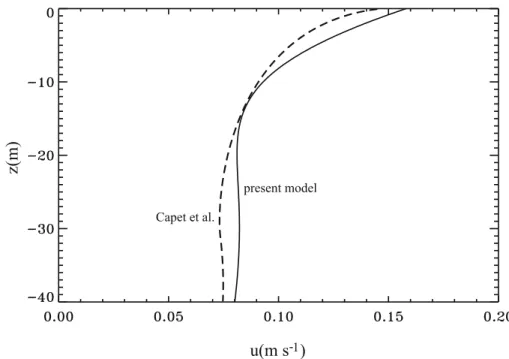
Sg ≈5×10−4s−1, A≈5×10−2ms−1, δE ≈10m, h∼40m (12b)

15

Once (12b) are substituted in Eq. (8e), one computesKe defined in (Eq. 6d) while the kinetic energyKE is computed from Fig. 10 of C8. WithK andKe, one then computes

λ, ηdefined in Eq. (7b); as for the buoyancy frequencyN, we take the characteristic mixed layer value of N=₁₀−3_s−1_{. In Fig. 1 we compare the profile of} ₋_∂_z_FT

V (z) from

Eq. (11a) with that of Fig. 12 of C8 (black dashed line). In Fig. 2, we compare the

20

profiles of the fluxesF_VT(z)from the present model:

F_VT =_ηδ_E_A_{₍₁₋_eζ_cos_ζ₋_{ζ /ζ}₀₎₋_λ_[_eζ_sin_ζ+1

2A

−1_Sg_ζ₍_z₋_z

0)]} ∇HT

(12c)

(22)

OSD

6, 2157–2192, 2009

model

Title Page

Tables Figures

◭ ◮

Back Close

Full Screen / Esc

Interactive Discussion the mixed layer depth. As for the profile of−∂_zF_VT(z), they are quite close in the upper

half of the mixed layer but diff_{er somewhat in the lower half. We think this is due}

to the similarity of the mean velocity profile Eq. (8a, c) with that in the C8 at small depths and by an unavoidable diff_{erence in the lower part of the mixed layer due to the}

diff_{erent profiles of the vertical viscosity used here and in the C8 simulations. Though}

5

in our analysis we adopted the Ekman profile of the mean velocity which correspond to ν(z)=_{const. while C8 adopted a more realistic model for} _ν₍_z_{), the profiles} _|u(z)|

compare well, as seen in Fig. 3. We carried out a further test the model: we used Eq. (10b) to computeKE averaged over the mixed layer. The results, compared with

the value of C8 in their Fig. 10, are:

10

K_E(model)≈1.6·10−3m2s−2, K_E(C8)≈2.10−3m2s−2 (12d) which are quite close. On the other hand, from Eq. (12b) we obtain the Ekman ki-netic energy (which yields the main contribution to the ML baroclinic mean energy)

e

K≈1.25·10−3m2s−2. Thus condition Eq. (6c) of the applicability of the model is satis-fied.

15

9 No-wind case

In addition to the case studied by C8, there are also data from simulations correspond-ing to the less realistic case of no wind (Fox-Kemper et al., 2008, hereafter FFH) which we consider since they serve the purpose of an additional test of our model predictions. Following FFH, we assume that the mean velocity is in a thermal wind balance with the

20

mean buoyancy field and that the mean buoyancy gradient does not vary inside the mixed layer, i.e. u_z=_f−1e_z×∇Hb isz independent. Irrespectively of the surface value

ofu, from the second of Eq. (7f) and the first of Eq. (7d), we derive that:

e

u= 1

2f(2z+h)ez× ∇Hb, ub=

1

(23)

OSD

6, 2157–2192, 2009

model

Title Page

Tables Figures

◭ ◮

Back Close

Full Screen / Esc

Interactive Discussion Takingτ=_b_{in Eq. (7e, f), and using Eq. (13a), the buoyancy flux is given by:}

F_V(z)=_a₍₁₋_ξ2₎_|∇_H_b_|2_, _ξ=₁+₂_zh−1_, _a=h

2

4f

x3/2y

(1+_x₎₍₁+_x+_y2₎ (13b)

with:

FV(0)=0, FV(−h)=0, FV(−h/2)=a

∇Hb

2>0 (13c)

The baroclinic mean kinetic energyKe near the surface is obtained from its definition in

5

Eqs. (6f) and (13a):

e

K = 1

8h 2_f−2_|∇

Hb|2 (13d)

As for the dimensionless variable y defined in Eq. (7b), it is easy to express it in terms of the Richardson number Ri corresponding to a geostrophic mean velocity (ℓf π=_hN_):

10

y2= N

2

h2 π2_Ke

= 8

π2Ri, Ri=N 2_f2_/_|∇

Hb|2 (14a)

To solve equation Eq. (7j) forK_E, we findV from Eq. (7k) with the result:

V = h

12fe× ∇Hb (14b)

Substituting this relation into Eq. (7j), using Eq. (7b), we obtain the following relation forxand its solution:

15

4 3C

3/2_y2₌

(1+_x₎₍₁+_x+_y2₎_, _x = KE

e

K

= 9Ri−

p

Ri2+₂₆_._4Ri

Ri+p_Ri2+₂₆_._4Ri

(24)

OSD

6, 2157–2192, 2009

model

Title Page

Tables Figures

◭ ◮

Back Close

Full Screen / Esc

Interactive Discussion whereC=_{2.5. Recall that the model prediction Eq. (7e,f) and, therefore, Eq. (13b) are}

applicable under condition Eq. (6c), i.e.

x≥1 Ri≥1.5 (14d)

From the second of Eq. (14c), we further obtain that the limit Ri→∞ corresponds to

xmax≈4. Substituting the first of Eq. (14c) into the last of Eq. (13b) together with the

5

first of Eq. (13a), we obtain:

a=₀_.₀₆_|_f_|−1_h2Φ_(Ri)_, Φ_(Ri)=_x3/2_Ri−1/2 _(14e)

The first of Eq. (13b) then becomes:

FV(z)=0.06|f|−1h2(1−ξ2)|∇Hb|2Φ(Ri), ξ=1+2zh−1 (14f)

To compare Eq. (14f) with the FFH data, we recall that in their Fig. 14e the authors

10

plotted the ratio:

Λ_(data)= FV(data)

F_V(FFH), 5<Ri<10 3

(15a)

where:

FV(FFH)=0.06|f|−1h2µ(z)|∇Hb|2, (15b)

µ(z)=₍₁₋_ξ2₎₍₁+₅_ξ2_/₂₁₎ _(15c)

15

is the parameterization suggested by FFH. Even though the simulation data exhibit a scatter by more than in order of magnitude, FFH interpret the lineΛ =_{1 representing}

their model, to be in agreement with the data. To compare our model results with the same simulation data, we construct the ratio:

Λ_(model)= FV(present model)

F_V(FFH) 5<Ri<10 3

(15d)

(25)

OSD

6, 2157–2192, 2009

model

Title Page

Tables Figures

◭ ◮

Back Close

Full Screen / Esc

Interactive Discussion To compute Eq. (15d), we notice that the profileµ(z) in Eq. (15c) has the additional

factor (1+₅_ξ2_/_{21) in comparison with the profile Eq. (14f). The di}ff_{erence does not}

exceed 25% and it is due to the coarse approximation we used in the integration of Eq. (7a) over z as we discussed below Eq. (7d). Neglecting the additional factor, we substitute Eqs. (14f) and (15b,c) into Eq. (15d) and obtain:

5

Λ_(model)= Φ_(Ri) _(15e)

whereΦ_{(Ri) is given in Eq. (14f, e) which we recall is valid for Ri}_>_{1.5. Inspection of}

Fig. 4 shows that in the Ri interval where the simulation data are available, the FFH and present model are consistent.

Finally, we discuss whether the FFH flux formula Eq. (15a,b) without wind can

rep-10

resent the case with wind. To that end, we take the value ofS_g in the first of Eq. (12b) as determined from C8 simulations and substitute it in Eq. (11b). The result is:

∇Hb≈0.5×10−7s−2 (15f)

Substituting this result in Eq. (15b, c), and using the same mixed layer depthh=_{40 m}

as in C8, we obtain:

15

maxFV(FFH)=2.4×10−9m2s−3 (15g)

If one compares this value with the realistic value from C8 (Fig. 2):

maxF_Vb=_gα_T_max_FT

V =2·10

−8_m2_s−3 _(15h)

one concludes that the FFH flux formula underestimates the true flux by about an order of magnitude. Our results confirm the conclusion of Mahadevan and Tandon (2006)

20

that “winds plays a crucial role in inducing submesoscale structure”.

10 Conclusions

(26)

OSD

6, 2157–2192, 2009

model

Title Page

Tables Figures

◭ ◮

Back Close

Full Screen / Esc

Interactive Discussion is still incomplete, numerical simulations of increasingly higher resolution have been

a rich source of information that serves as a test bed for parameterizations of the sub-mesoscale fluxes to be then used in low resolution OGCMs to represent structures they cannot resolve. If one considers that the highest resolution of about 1/10◦ stand alone OGCMs can resolve structures of about 10 km size which is 10 times larger than

sub-5

mesoscale sizes and that OGCMs employed in thousand years runs for climate studies can hardly aff_{ord even a 1}◦_{resolution which corresponds to structures 100 times larger}

than sub-mesoscales, one realizes that a good deal of important physical processes have thus far gone unrepresented in low resolution OGCMs.

The present paper presents a model of the key unresolved quantity in the dynamic

10

equations, namely the vertical flux of an arbitrary tracer which we express in terms of the resolved fields. The results can be applied to the equations for the mean T

(temperature), S (salinity) and C(passive scalar such as Carbon). The key relations are given by Eq. (7a, b, j, k), is to be used in OGCMs that resolve mesoscales but not sub-mesoscales. The model predictions have been tested against the results of

15

sub-mesoscale resolving simulations. In future work we shall derive expressions for the tracer vertical flux to be used in OGCMs that do not resolve either submesoscales or mesoscales.

Appendix A

20

The non-linear termsQH

As discussed in textbooks on Turbulence theories (e.g., Batchelor, 1970; Lesieur, 1990; McComb, 1992), the stochastic Langevin equation has played a major role in turbu-lence modeling studies (Kraichnan, 1971; Leith, 1971; a review can be fund in Herring and Kraichnan, 1971; Chasnov, 1991). Though most turbulence models are presented

25