THE LOW PRICE EFFECT ON THE POLISH MARKET

THE LOW PRICE EFFECT

ON THE POLISH MARKET

Adam Zaremba*

, Radosław Żmudziński**

Introduction

he low price efect is probably the oldest anomaly observed in the inancial markets. Simplifying it implies that the lower the nominal stock price, the higher the expected return. It was irst observed by Fritzmeier (1936). His computations were frequently repeated and extended. he aim of our paper is to further investigate the low price efect, its sources and characteristics.

Our research broadens academic knowledge in a few ways. Firstly, we deliver some fresh evidence on the low price efect in Poland - the biggest and most liquid market in Eastern Europe, and one which has not been analyzed in a comprehensive way so far.

Secondly, we analyze the interdependence among the low price efect and other rate of return factors such as: liquidity, value and size. hirdly, we investigate whether the low price efect is present ater accounting for liquidity. Fourthly, we check whether the efect is robust to transaction costs. Our basic hypotheses are that the low price efect is present on the Polish market and additionally it can be ampliied by combining it with other factors, however it only compensates investors for transaction costs and illiquidity.

he paper is opened with an introduction, which is followed by four sections. In the irst section, we review the existing literature on the low price efect.

In this paper we investigate the characteristics of the low price anomaly, which implies higher returns to stocks with a low nominal price. The research aims to broaden academic knowledge in a few ways. Firstly, we deliver some fresh evidence on the low price efect from the Polish market. Secondly, we analyze the interdependence between the low price efect and other return factors: value, size and liquidity. Thirdly, we investigate whether the low price efect is present after accounting for liquidity. Fourthly, we check to see whether the low price efect is robust to transaction costs. The paper is composed of three main sections. In the beginning, we review the existing literature. Next, we present the data sources and research methods employed. Finally, we discuss our research indings. Our computations are based on all the stocks listed on the Warsaw Stock Exchange (WSE) in the years 2003-2013. We have concluded that the low price efect is present on the Polish market, although the statistical signiicance is very weak and it disappears entirely after accounting for transaction costs and liquidity.

Received: 04.01.2014 Accepted: 28.04.2014

G11, G12, G14

low price efect, Warsaw Stock Exchange, Polish market, stock market anomaly

Abstract

Next, we present the data sources and research methods employed. Finally, we discuss our research results. Our research is based on all the stocks listed on the Warsaw Stock Exchange (WSE) in the years 2003-2013. he last part of the paper includes concluding remarks and indication for further research.

Low price effect in

international markets

he low price efect was initially documented in the USA by Fritzmeier (1936). He observed that the low-priced stocks were characterized by higher returns. However, the bigger proits come not without a higher risk: the stocks were also more variable. hese indings were later partly contradicted by Allison and Heinds (1966) and Clenderin (1951) who found that the source of the price risk was actually not the low price but the low “quality” of stocks perceived by investors. In other words, the low-priced good-quality stocks did not show exceptional price risk. Later research concentrated mainly on U.S. markets. Pinches and Simon (1972) tested portfolio strategies based on selection of low-priced stocks on the AMEX. he returns turned out to be particularly high. he initial computations of Fritzmeier (1936) were also conirmed by Blume and Husic (1973), which additionally investigated the beta variability. hey found that in the time-series approach, the beta seems to be negatively correlated with the stock price. Some interesting research was conducted later by Bar-Yosef and Brown (1979) and Strong (1983). hose researchers noticed that the low price efect is valid only for companies which split their shares. hese indings correspond with later frequent event-studies of splits and analyses of post-split abnormal returns (Ikenberry, Rankine & Stice 1996; Desai & Jain 1997), which document positive post-split price drit. Bachrach and Galai (1979) came to the conclusion that the low price is probably a surrogate for an unspeciied economic factor. he authors compared the performance of under- and over-20 dollars per share companies and found that the systematic risk did not fully explain the superior returns of the cheaper stocks. Similar research was later conducted by Christie (1982) and Dubofsky and French (1988), who used a diferent risk measure. hey documented how low price stocks are actually more volatile, which in part could be explained by the degree of leverage. Edminster and Greene (1982) scrupulously classiied stocks into as many as 60 various categories divided by

their share price. he low-priced stock outperformed most other share-classes.

he superior performance of cheap stocks was also conirmed by Goodman and Peavy (1986), who additionally showed that the anomaly is robust to a few other determinants of variations in cross-sectional stock returns: size premium and earnings yield efect.

Branch and Chang (1990) linked the low price anomaly with the research on seasonal patterns in the stock market. hey found that the low price shares are particularly likely to outperform in January and exhibit poor returns in December.

Among the latest studies, it is important to mention the extensive research of Hwang and Lu (2008). heir study examines the cross-sectional efect of the nominal share price. he indings indicate that share price per se matters in cross-sectional asset pricing: stock return is inversely related to nominal price. he authors show that a strategy of buying penny stocks can generate a signiicant alpha even ater considering the transaction costs. hese abnormal returns are robust in the presence of other irm characteristics such as size, book-to-market equity, earnings/price ratio, liquidity and past returns.

he international evidence of the low price anomaly outside the USA is rather modest, but some interesting examples could be found. For instance, Gilbertson et al. (1982) documents the efect on the 1968-1979 sample on the Johannesburg Stock Exchange (SAR). However, these results are somehow mixed, as they are contradicted by the later research of Waelkens and Ward (1997).

he low price efect has not been investigated in the Polish market so far, therefore this is an interesting gap to explore.

Research methods and data

sources

We investigate the issue of low-priced stock returns on the Polish market on a sample of all stocks listed on the Warsaw Stock Exchange between 09/25/2003 and 09/25/2013. he data came from Bloomberg. We used both listed and delisted stocks in order to avoid the survivorship bias. All the computations were performed before and ater inclusion among stocks traded on NewConnect.

all four computable characteristics in a given year. Additionally, we compute three additional factors for all the stocks. We chose size, value and liquidity factors as they are well documented in US and international stock returns.

he factors are deined as follows:

1) value factor (V) – the book value to market value ratio (BM/VM) at the time of portfolio formation,

2) size factor (S) – the total market capitalization of a company at the time of portfolio formation,

3) liquidity factor (L) – the average trading volume over the last month multiplied by the current price.

he number of stocks in the sample grew along with the development of the Polish capital market from 61 in the beginning of the research period to 476 in the end including the NewConnect stocks, and from 61 to 364 excluding them. Based on the P, we construct three separate portfolios including 30% of stocks with the lowest price, 30% of stocks with the highest price and the remaining 40% of the mid-stocks. We use three diferent weighting schemes. he irst type of portfolios are equal weighted, which means that each stock at the time of formation participates equally in the portfolio. he second scheme is capitalization weighting, which means that the weight of each stock is proportional to the total market capitalization of the company at the time of portfolio formation. he last scheme is liquidity weighting. As a proxy for liquidity we use zloty volume, which is the time-series average of daily volumes in a month preceding the portfolio formation multiplied by the last closing price (actually the same as L). he reason we use liquidity weighting is that a lot of stocks in the emerging markets tend to be signiicantly illiquid. As a result of that, the regular reconstruction and rebalancing of equal or capitalization weighted portfolios may be completely unrealistic. he liquidity weighted portfolio is the one which is the easiest to reconstruct and rebalance within a market segment. In other words, by using the liquidity weighted portfolios we avoid the illiquidity bias, which may arise due to some inherent illiquidity premium linked to illiquid companies. he participation of such companies in equal and capitalization weighted portfolios may be artiicially overweighed to some artiicial level, which cannot be achieved by a real investor. hus, liquidity weighting is far better aligned with a true investor’s point of view, as it avoids the impact of “paper” proits from illiquid assets.

It is also important to point out, that the liquidity weighting does not deal with the issue of an illiquidity premium entirely, as some securities with similar characteristics (like high P stocks) may be illiquid as a group and thus bear some illiquidity premium. Nonetheless, this research takes a point of view of an individual investor with a medium-size portfolio, for whom such a group illiquidity does not pose a problem. he detailed analysis which would take advantage of some more sophisticated price impact function to account for illiquidity, is beyond the scope of this paper.

Along with the price portfolios, we also calculate returns on the market portfolio, by which we mean the portfolio of all the stocks in the sample. For better comparison, we compute the market portfolios each time using the same methodology as for the price portfolios. In other words, we compute three diferent market portfolios: equal, capitalization and liquidity weighted. he price and market portfolios are reconstructed and rebalanced once a year on the 25th of September. he date was chosen intentionally in order to avoid look-ahead bias.

Next, we build fully collateralized market-neutral (MN) long/short portfolios mimicking the behavior of the low-price-premium factor. he portfolio is 100% long in low-priced stocks, 100% short in high-priced stocks and 100% long in a risk free asset. We employ a WIBOR’s bid, as a proxy for its yield. In other words, we assume that an investor invests all his money in the risk free assets, and additionally sells short the high-priced stocks and invests all the proceedings in the low-priced stocks. Additionally, we build similar portfolios for Fama-French factors (Fama & French 1993): V, S. hese portfolios are later used in additional correlation analysis. he MN portfolios’ construction are based on existing theoretical and empirical evidence in the ield, so as to make them positively exposed to factor-related premiums. In other words, the portfolios are always long in the 30% of stocks, which yields the highest risk-adjusted returns, short in the 30% of stocks which yields the lowest risk-adjusted returns, and 100% long in a risk-free asset. As a result, we create 2 distinct portfolios:

2) size market neutral long/short mimicking portfolio (“size MN”), which is 100% long in the 30% smallest companies, 100% short in the 30% biggest companies and 100% long in a risk-free asset.

Again, as in the previous case, the stocks in the portfolios are weighted according to three diferent schemes: equal, capitalization-based and liquidity-based.

Finally, the performance of the long/short portfolios is tested against two models: the market model and CAPM (Cambell, Lo & MacKinlay, 1997; Cochrane 2005). Here, we base our computations on log returns. he irst one was the classical market model.

R

₌

_α

₊

_β

R

₊

_ε

, (1)

E

ε

( )

=

0

,

var

( )

ε

=

σ

2

,

where Rit and Rmt are the period-t returns on the security and the market portfolio, εitis the zero mean disturbance term and αi, βiand σε^2are the parameters of the market model. In each case, we computed the proxy for the market portfolio based on a cross-sectional average of all stocks in the sample using the same weighting scheme as for the factor portfolios. his means that dependent on the construction of factor portfolios the market portfolio is either equal, capitalization or liquidity weighted. he other model we employ is the Capital Asset Pricing Model. he long/short portfolios’ excess returns were regressed on the market portfolio’s excess returns, according to the CAPM equation:

R

−

R

=

α

+

β

(

R

−

R

)

+

ε

(2)

where R_pt,R_mt and R_t are annual long/short portfolio, market portfolio and risk-free returns, and α_i and β_i

are regression parameters. We used WIBOR’s bids to represent the risk-free rate. he α_i intercept measures the average annual abnormal return (the Jensen-alpha). In both models, our zero hypothesis is that the alpha intercept is not statistically diferent from zero, and the alternative hypothesis states that it is actually diferent from zero. We ind the equation parameters using OLS and test them in parametric way.

Having tested the sole price-portfolios performance, we analyze the interactions between price and other factor premiums. First, for presentational purposes,

we computed time-series correlation matrices of the MN Fama-French factor portfolios and low-high price portfolio. Next, we provide more formal statistical inferences. At this stage, all the computations are based on equal weighted portfolios. We divide the stocks into separate groups based on combinations of P and other fundamental characteristics described above: V, S and L. We do it as follows. Firstly, we ascribed each stock to one of the subsamples based on the fundamental factors above: low 30%, mid 40% or high 30%. In other words, we segregated all the stocks into low, medium or high P, low, medium or high S, low, medium or high V, and low, medium or high L. Secondly, we create nine portfolios for each pair combination of two of the mentioned fundamental factors. For instance, in the case of pair V+P, we created a low V and low P portfolio, which consisted of stocks that belonged simultaneously to the low V subgroup and low P subgroup; a low V and medium P portfolio, which consisted of stocks that belonged simultaneously to the low V subgroup and medium P subgroup; and so on for 7 other V+P portfolios. We do the same in the cases of other pair combinations (V+P, L+P, S+P), so inally we arrive with 27 portfolios.

Next, we construct collateralized market-neutral long/short portfolios for each of the pair combinations. he premises of certain long/short portfolios are based on existing previous theoretical and empirical evidence. hus, we create the following equal weighted portfolios:

• 100% long high V and low P, 100% short low V and high P, 100% long risk-free asset;

• 100% long low S and low P, 100% short high s and high P, 100% long risk-free asset;

• 100% long low L and low P, 100% short high L and high P, 100% long risk-free asset.

For example, the irst long/short portfolio is 100% long the stocks which belong at the same time to the high value and low price subgroups, 100% short the stocks which belong at the same time to the low value and high price subgroups, and 100% long in the risk-free asset. Finally, we test the described portfolios using identical procedures as described above against the market model and the CAPM.

f p

_{( )}

= ×

k

p

, (3)

where p is the stock price at the time of portfolio formation and k is the constant cost component. As the proxy for the k we use half of the quoted spread, which is deined as:

k

₌

1

_×

k

2

where:

k

P

P

P

Q ask j t bid j t

mid j t ,

, , , ,

, ,

=

−

and P_ask,j,t, P_bid,j,t and P_mid,j,tare ofer, bid and mid prices of stock j at time t. Using the

k

Next, we compute simpliied post-cost returns by employing the following formula:

R

=

R

−

(

k

+

k

)

0 1 , (6)

where

k

0 and

k

(halves of the quoted spreads) at the beginning and at the end of the measurement period. In other words, we take a simpliied approach by assuming an equal 100% turnover rate in all portfolios. Finally, using the post-cost returns and log returns, we repeat all the computations and statistical interfering in the same way as for the raw pre-cost returns. It is important to emphasize, that all the portfolios’ returns, including the market portfolio’s return, are computed based on post-cost returns. We do so in order to avoid the problem of comparing apples and oranges during the analysis.

Results and findings

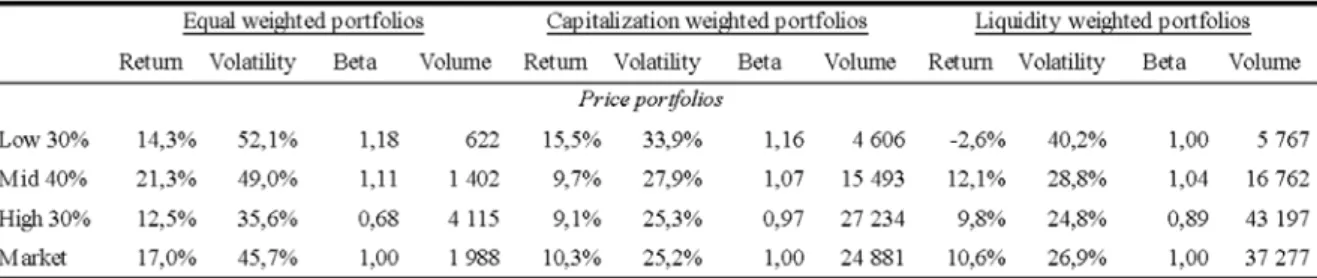
Table 1 presents pre-cost returns of price-sorted portfolios. he computation of equal weighted portfolios shows that with and without NewConnect stocks our indings indicate that the low price efect in the Polish market is virtually non-existent. However, it is not completely true when it comes to value

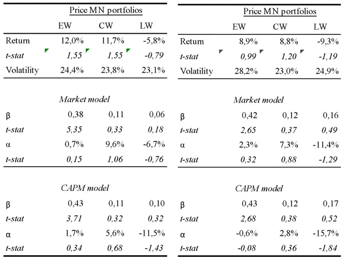
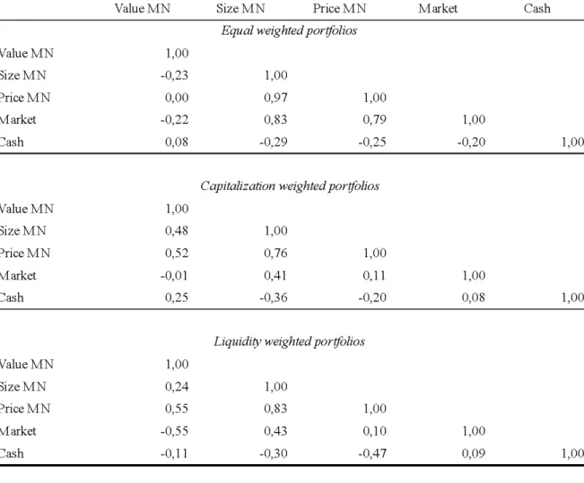
weighting. In the case of exclusion of NewConnet, the bottom 30% portfolio delivered 6,4 p.p. higher returns than the high 30% portfolio and 5,2 p.p. better results than the market portfolio. Unfortunately, the lower the price, the bigger the risk, both in beta or standard deviation terms. What is more, the price factor premiums turned out to be not robust to liquidity weighting. he premiums are actually inversed and the high price portfolio yields vividly better returns than the low price portfolios when liquidity weighting is applied, and additionally lower risk. hese results were generally conirmed by the analysis of collateralized market-neutral price-factor mimicking portfolios, although these results clearly lack statistical signiicance. his fact may be due tothe relatively short time-series in the young Polish market, but it may as well indicate that the price factor is non-existent. he price sorted portfolios yielded positive returns and positive market-model alphas, when we use equal and value weighting schemes and do not include NewConnect in the sample. However, ater adjusting the weights for the stocks’ individual liquidity, all the returns and risk-adjusted returns the price factor become negative. Summing up, it seems that on the Polish marketthe price premium – provided that it actually exists - is not immune to the question of stock liquidity. In fact, ater adjusting for liquidity, the factor premium seems to disappear. Table 3 exhibits time-series correlations among the MN factor mimicking portfolios. What is interesting is that the correlations are highly dependent on the weighting scheme. he high correlation with the small-cap factor is particularly worth noticing. Table 4 depicts some interactions of equal-weighted factor portfolios. Careful analysis suggests that the price factors actually do not exhibit any interactions with other factors. hey neither amplify nor contradict each other. Although Table 5 actually indicates some positive returns for the factor combination portfolios, these indings should not be taken too seriously. On the one hand, they are not statistically signiicant, on the other hand the positive returns or alphas may be ascribed rather to value, liquidity or size premium rather than the price factor.

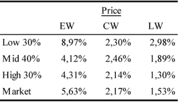
portfolios were signiicantly higher than for the capitalization (CW) and liquidity weighted (LW) portfolios. In the case of the entire market portfolio, the EW was equal to 5,63% without NewConnect and 7,36% with NewConnect, and in the case of LW it was over 3 times less – 1,53% excluding NewConnect and 1,57%. his situation is due to very large spreads among the smallest and least liquid stocks. Another interesting observation is the fact that the spreads among the low price stocks were actually 2-3 times higher than in the case of the high price stocks. his observation contradicts the reasoning that the stock splits increase the liquidity and decrease the trading costs. his phenomenon was actually documented and analyzed in the recent inancial literature (Weld et al. 2009).

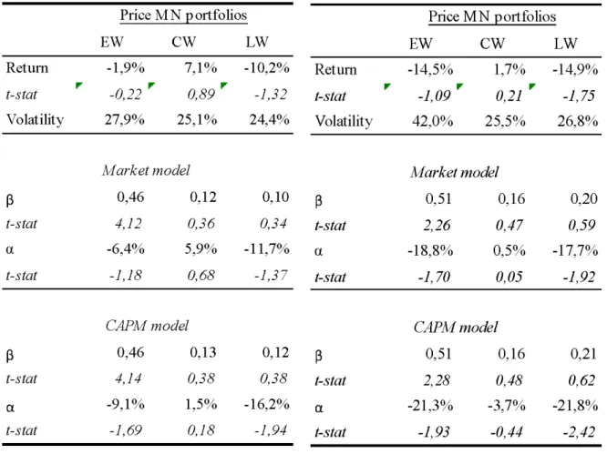
Table 7 depicts the post-cost returns of the price sorted portfolios. Analyzing the table, we can draw a few interesting conclusions. First, the transaction costs completely kill the already equal and liquidity weighted portfolios. Second, the high NewConnect spreads cause the premium in capitalization weighted portfolios to disappear. In other words, it seems that the transaction costs are on this market so high that they cannot be compensated with the price premium. he only survivor among various markets and weighting schemes are actually the capitalization weighted portfolios before inclusion of NewConnect shares into the sample. In this case, the low price portfolio yielded remarkably better return than the market and high price portfolios, although it coincided with higher risk. hese observations are generally conirmed by the analysis of the returns of the post-cost market-neutral price-factor mimicking portfolios (Table 8). Aside from the CW portfolio without NewConnect shares, all the portfolio average returns become negative. Similarly, all the alphas – both in market and CAPM models – turn negative and some of them are even quite signiicant from the statistical point of view. he only exception is the CW non-NewConnect portfolio, although even in this case the results are not statistically signiicant at any reasonable level.

Conclusions and areas for

further research

In this paper we conduct research on the low price efect on the Polish market. he analysis allows us to draw a few interesting conclusions and answer the initial questions stated in the beginning of the paper.

First, the evidence suggests that the low-price efect exists, but the formal statistical signiicance is rather weak. We observe the superior performance of low price shares only in the case of equal and capitalization weighted portfolios without NewConnect shares. What is more, the abnormal returns are not statistically signiicant. In other words, our indings do not conirm the results obtained by Fritzmeier (1936) and his followers. Second, we do not ind any interesting interactions between price and other factors. Again, it is contrary to the previous research by, for example, Goodman and Peavy (1986). hird, we check whether the factor premiums are robust to liquidity. hey are deinitely not. Ater adjusting the factor portfolio weights for liquidity, the superiority of low-priced stocks completely evaporated. Fourth, we investigated the impact of transaction costs on low price premiums. he only portfolio which yielded abnormal returns – the cap-weighted portfolio with NewConnect stocks excluded – remained superior. Finally, when we account for both the liquidity and transaction costs, the superiority of low-priced stocks ceased to exist. hese indings are not contradictory to the reasoning of Hwang and Lu (2009). Summing up, our observations do not conirm the indings from the developed markets and the evidence for the low price premium in Poland is rather weak.

superior, statistically signiicant, returns on low price stocks in Poland should be investigated. Our indings do not conirm most of the basic observations in the

developed markets and the reasons for this remain unknown.

References

Allison, S.L., Heins, A.J. (1966). Some Factors Afecting Stock Price Variability. Journal of Business, vol. 39, no. 1, p. 19-23.

Almgren, R., hum, C., Hauptmann, E., Li, H. (2005). Equity Market Impact, Risk, July.

Amihud, Y., Mendelson, H., Lauterbach, B. (1997). Market Microstructure and Securities Values: Evidence from the Tel Aviv Stock Exchange. Journal of Financial Economics,

vol. 45, p. 365-390.

Asness, C.S., Moskowitz, T.J., Pedersen, L.H. (2013). Value and Momentum Everywhere. he Journal of Finance, vol. 68, no. 3, p. 929–985.

Bachrach, B., Galai, D. (1979). he risk-return Relationship and Stock Prices. Journal of Financial and Quantitative Analysis, vol. 14, no. 2, p. 421-441.

Bar-Yosef, S., Brown, L.D. (1979). Share Price Levels and Beta. Financial Management, vol. 8, no. 1, p. 60-63.

Blume, M. E., Husic, F. (1973). Price, Beta and Exchange Listing. Journal of Finance, vol. 28, no. 2, p. 283-299.

Branch, B., Chang, K. (1990). Low Price Stocks and the January Efect. Quarterly Journal of Business and Economics, vol. 29, no. 3, p. 90-118.

Breen, W.J., Hodrick, L. S., Korajczyk, R.A. (2002). Predicting Equity Liquidity. Management Science, vol. 48, p. 470–483.

Brennan, M. J., Subrahmanyam, A. (1996). Market Microstructure and Asset Pricing: On the Compensation for Illiquidity in Stock Returns. Journal of Financial Economics, vol. 44, p. 441-464.

Cambell, J.Y., Lo, A. W., MacKinlay, A.C. (1977). he Econometrics of Financial Markets, Princeton University Press, Princeton, New Jersey, USA.

Carhart, M.M. (1977). On Persistence in Mutual Fund Performance. Journal of Finance, vol. 52, p. 57–82.

Chan, H., Fa, R. (2005). Asset Ricing and the Illiquidity Premium.he Financial Review, vol. 40, p. 429-458.

Chan, L.K.C, Hamao, Y, Lakonishok, J. (1991). Fundamentals and Stock Returns in Japan. Journal of Finance, vol. 46, p. 1739-1764.

Chriestie, A.A. (1982). he Stochastic Behavior of Common Stock Variances – Value, Leverage and Interest Rate Efects. Journal of Financial Economics, vol. 10, no. 4, p. 407-432.

Clenderin, J.C. (1951). Quality Versus Price as Factors Inluencing Common Stock Price Fluctuations. Journal of Finance, vol. 6, no. 4, p. 398-405.

Cochrane, J.C. (2005). Asset Pricing, Princeton University Press, Princeton, New Jersey.

Desai, H., Jain, P.C. (1997). Long-run Common Stock Returns Following Stock Splits and Reverse Splits. Journal of Business, vol. 70, p. 409–433.

Dubofsky, D. A., French, D.W. (1988). Share Price Level and Risk: Implications for Financial Management.

Managerial Finance, vol. 14, no. 1, p. 6-9.

Edminster, R. O., Greene, J.B. (1980). Performance of Super-low-price Stocks. Journal of Portfolio Analysis, vol. 7, no. 1, p. 36-41.

Fama, E. F., French, K.R. (2012). Size, Value, and Momentum in International Stock Returns. Journal of Financial Economics, vol. 105, no. 3, p. 457-72.

Fama, E. F., French, K.R. (1992). he Cross-section of Expected Stock Returns. Journal of Finance, vol. 47, p. 427-466.

Fama, E. F., French, K. R. (1998). Value versus Growth: he International Evidence. Journal of Finance, vol. 53, p. 1975-1999.

Fama, E. F., French, K.R. (1993). Common Risk Factors in the Returns on Stocks and Bonds. Journal of Financial Economics, vol. 33, p. 3-56.

Fritzmeier, L.H. (1936). Relative Price Fluctuations of Industrial Stocks in Diferent Price Groups. Journal of Business, vol. 9., no. 2, p. 133-154.

Gharghori, P., Lee, R., Veeraraghavan, M. (2009). Anomalies and Stock Returns: Australian Evidence.

Accounting & Finance, vol. 49, no. 3, p. 555–576.

Gilbertson, R.A.C, Afeck-Graves, J. F., Money, A.H. (1982). Trading in Low Priced Shares: an Empirical Investigation 1968-1979, vol. 19, p. 21-29.

Glosten, L.R., Harris, L.E. (1988). Estimating the Components of the Bid/ask Spread. Journal of Financial Economics, vol. 21, p. 123–142.

Goodman, D. A., Peavy III, J.W. (1986). he Low Price Efect: Relationship with other Stock Market Anomalies.

Review of Business and Economics Research, vol. 22, no. 1, p. 18-37.

Herrera, M. J., Lockwood, L.J. (1994). he Size Efect in the Mexican Stock Market. Journal of Banking and Finance,

Heston, S.L., Rouwenhorst, K. G., Weessels, R.E. (1999). he Role of Beta and Size in the Cross-section of European Stock Returns. European Financial Management, vol. 5, p. 9 -27.

Hu, A.-Y. (1997). Trading Turnover and Expected Stock Returns: he Trading Frequency Hypothesis and Evidence from the Tokyo Stock Exchange, SSRN working paper, online: http://papers.ssrn.com/sol3/papers.cfm?abstract_ id=15133 [download date: 12/05/2013].

Hwang, S., Lu, C. (2008). Is Share Price Relevant? Working paper, available at SSRN, online: http://papers.ssrn.com/ sol3/papers.cfm?abstract_id=1341790 [download date: 12/04/2013].

Ikenberry, D., Rankine, G., Stice, K. (1996). What Do Stock Splits Really Signal? Journal of Financial and Quantitative Analysis, vol. 31, p. 1-18.

Korajczyk, R. A., Sadka, R. (2004). Are Momentum Proits Robust to Trading Costs? he Journal of Finance, vol. 59, no. 3, p. 1039-1082.

Lam, K.(2002). he Relationship between Size, Book-to-market Equity Ratio, Earnings–price Ratio and Return for the Hong Kong Stock Market. Global Finance Journal, vol. 13, no. 2, p. 163-179.

Pinches, G. E., Simon, G.M. (1972). An Analysis of Portfolio Accumulation Strategies Employing Low-priced Common Stock. Journal of Financial and Quantitative Analysis, vol. 7, no. 3, p. 1773-1796.

Rouwenhorst, K.G. (1999). Local Returns Factors and Turnover in Emerging Stock markets. Journal of Finance,

vol. 54, p. 1439- 1464.

Strong, R.A. (1983). Do Share Price and Stock Splits Matter? Journal of Portfolio Management, vol. 10, no. 1, p. 58-64.

Waelkens, K., Ward, M. (1997). he Low Price Efect on the Johannesburg Stock Exchange, Investment Analyst Journal, vol. 45, p. 35-38.

Tables

Table 1: Pre-cost price-sorted portfolios

Table presents the pre-cost return characteristics of price portfolios. Portfolios are sorted according to share prices in the year preceding the portfolio formation (“price”). “Return” is the average annual geometric rate of return, “volatility” is an annual standard deviation of log returns, “beta” is regression coeicient calculated against a deined market portfolio and “volume” is a cross-sectional weighted-average of single stocks’ time-series weighted-averaged daily trading volumes in the month preceding the portfolio formation multiplied by the stock price. he liquidity

weighted portfolios were weighted according to the “volume” deined as above. he market portfolio in each case is built using the same methodology as the remaining portfolios, which means it is either equal, capitalization or liquidity weighted. he data source is Bloomberg and the computations are based on listings of Polish companies during the period 09/25/2003-09/25/2013. Panel A depicts the results excluding NewConnect stocks and Panel B ater their inclusion.Model Summary and Parameter Estimates

Panel A: before inclusion of NewConnect stocks.

Table 2: Pre-cost market-neutral price-factor mimicking portfolios

Table 2 exhibits pre-cost return characteristics of the market-neutral factor mimicking portfolios. Portfolios are created based on share prices in the year preceding the portfolio formation (“price”). “Return” is the average annual geometric rate of return and “volatility” is an annual standard deviation of log returns. “EW”, “CW” and “LW” denotes equal-, capitalization- and liquidity-based weighting scheme. he liquidity weighted portfolios were weighted according to the “volume” deined as stocks’ time-series averaged daily trading volume in the month preceding the portfolio formation multiplied by the

stock price. α and β are model parameters computed in each case according to the model’ speciication. he market portfolios in each case are built using the same methodology as the remaining portfolios, which means they are either equal, capitalization or liquidity weighted. he data source is Bloomberg and the computations are based on listings of Polish companies during the period 09/25/2003-09/25/2013. If necessary, a 1-year bid for Warsaw Interbank Ofered Rate is employed as a proxy for a risk-free rate. Panel A depicts the results excluding NewConnect stocks and Panel B ater their inclusion.

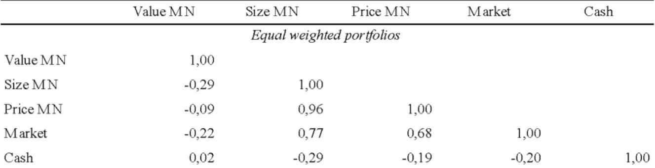
Table 3: Factor correlations

Table 3 exhibits Pearson’s correlation coeicients of pre-cost log returns among market neutral factor-mimicking portfolios, stock market portfolio (“market”) and yields in the cash market (“cash”). Portfolios are created based on price (“price”), BV/ MV (“value”) and company capitalization (“size”). he liquidity weighted portfolios were weighted according to the “volume” deined as stocks’ time-series averaged daily trading volume in the month preceding the portfolio formation multiplied by

the stock price. he market portfolios in each case are built using the same methodology as the remaining portfolios, which means they are either equal, capitalization or liquidity weighted. he data source is Bloomberg and the computations are based on listings of Polish companies during the period 09/25/2003-09/25/2013. Panel A depicts the results excluding NewConnect stocks and Panel B ater their inclusion.

Panel B: after inclusion of NewConnect stocks.

Table 4: Interactions between price and systematic risk factors

Table 4 presents pre-cost return characteristics of portfolios sorted simultaneously on two separate cross-sectional factors. All portfolios are equal weighted and created based on pairs of following variables: price (“price”), BV/MV (“value”), company capitalization (“size”) or average zloty volume (“liquidity”). “Return” is the average annual geometric rate of return and “volatility” is an annual standard

Panel A: before inclusion of NewConnect stocks.

Table 5: Market-neutral portfolios based on pairs of factors

Table 5 presents pre-cost return characteristics of portfolios created based simultaneously on two separate cross-sectional factors. All portfolios are equal weighted and price created based on(“P”) and following variables: BV/MV (“V”), company capitalization (“S”) or average zloty volume (“L”). he market portfolios in each case are built using the same methodology as the remaining portfolios,

which means they are all equal weighted. he data source is Bloomberg and the computations are based on listings of Polish companies during the period09/25/2003-09/25/2013. If necessary, a 1-year bid for Warsaw Interbank Ofered Rate is employed as a proxy for risk-free rate. Panel A depicts the results excluding NewConnect stocks and Panel B ater their inclusion.

Table 6: Bid-ask spreads

Table 6 presents average bid-ask spreads for factor and market portfolios. he spreads are computed as (P_ask-P_bid)/P_mid , where Pask, Pbid, Pmid denote consecutively the best available ofer, the best available ofer bid and the mid-prices at the time of portfolio formation. Portfolios are created based on share price levels (“price”). “EW”, “CW” and “LW” denotes equal-, capitalization- and liquidity-based weighting scheme. he liquidity weighted portfolios were weighted according to the “volume” deined as stocks’ time-series averaged daily trading volume

in the month preceding the portfolio formation multiplied by the stock price. he market portfolios in each case are built using the same methodology as the remaining portfolios, which means they are either equal, capitalization or liquidity weighted. he data source is Bloomberg and the computations are based on listings of Polish companies during the period 09/25/2003-09/25/2013. Panel A depicts the results excluding NewConnect stocks and Panel B ater their inclusion.

Panel A: before inclusion of NewConnect stocks.

Table 7: Post-cost price-sorted portfolios

Table 7 presents the post-cost return characteristics of factor portfolios. Portfolios are sorted according share prices. “Return” is the average annual geometric rate of return, “volatility” is an annual standard deviation of log returns, “beta” is regression coeicient calculated against a deined market portfolio and “volume” is cross-sectional weighted-average of single stocks’ time-series weighted-averaged daily trading volumes in the month preceding the portfolio formation multiplied by the stock price. he liquidity

weighted portfolios were weighted according to the “volume” deined as above. he market portfolio in each case is built using the same methodology as the remaining portfolios, which means it is either equal, capitalization or liquidity weighted. he data source is Bloomberg and the computations are based on listings of Polish companies during the period 09/25/2003-09/25/2013. Panel A depicts the results excluding NewConnect stocks and Panel B ater their inclusion.

Panel A: before inclusion of NewConnect stocks.

Table 8: Post-cost market-neutral price-factor mimicking portfolios

Table 8 presents post-cost return characteristics of market-neutral factor mimicking portfolios. Portfolios are created based on share prices. “Return” is the average annual geometric rate of return and “volatility” is an annual standard deviation of log returns. “EW”, “CW” and “LW” denotes equal-, capitalization- and liquidity-based weighting scheme. he liquidity weighted portfolios were weighted according to the “volume” deined as stocks’ time-series averaged daily trading volume in the month preceding the portfolio formation multiplied by the stock price. α and β are model parameters computed

in each case according to the model’ speciication. he market portfolios in each case are built using the same methodology as the remaining portfolios, which means they are either equal, capitalization or liquidity weighted. he data source is Bloomberg and the computations are based on listings of Polish companies during the period 09/25/2003-09/25/2013. If necessary, a 1-year bid for Warsaw Interbank Ofered Rate is employed as a proxy for risk-free rate. Panel A depicts the results excluding NewConnect stocks and Panel B ater their inclusion.