www.ann-geophys.net/32/831/2014/ doi:10.5194/angeo-32-831-2014
© Author(s) 2014. CC Attribution 3.0 License.
Extreme ion heating in the dayside ionosphere in response to the
arrival of a coronal mass ejection on 12 March 2012
H. Fujiwara1, S. Nozawa2, Y. Ogawa3, R. Kataoka3, Y. Miyoshi4, H. Jin5, and H. Shinagawa5
1Faculty of Science and Technology, Seikei University, Tokyo, Japan
2Solar-Terrestrial Environment Laboratory, Nagoya University, Nagoya, Japan 3National Institute of Polar Research, Tokyo, Japan
4Department of Earth and Planetary Sciences, Kyushu University, Fukuoka, Japan 5National Institute of Communication Technology, Tokyo, Japan
Correspondence to:H. Fujiwara ([email protected])
Received: 28 February 2014 – Revised: 9 June 2014 – Accepted: 12 June 2014 – Published: 23 July 2014
Abstract. Simultaneous measurements of the polar iono-sphere with the European Incoherent Scatter (EISCAT) ul-tra high frequency (UHF) radar at Tromsø and the EISCAT Svalbard radar (ESR) at Longyearbyen were made during 07:00–12:00 UT on 12 March 2012. During the period, the Advanced Composition Explorer (ACE) spacecraft observed changes in the solar wind which were due to the arrival of coronal mass ejection (CME) effects associated with the 10 March M8.4 X-ray event. The solar wind showed two-step variations which caused strong ionospheric heating. First, the arrival of shock structures in the solar wind with enhance-ments of density and velocity, and a negative interplane-tary magnetic field (IMF)-Bzcomponent caused strong
iono-spheric heating around Longyearbyen; the ion temperature at about 300 km increased from about 1100 to 3400 K over Longyearbyen while that over Tromsø increased from about 1050 to 1200 K. After the passage of the shock structures, the IMF-Bzcomponent showed positive values and the solar
wind speed and density also decreased. The second strong ionospheric heating occurred after the IMF-Bz component
showed negative values again; the negative values lasted for more than 1.5 h. This solar wind variation caused stronger heating of the ionosphere in the lower latitudes than higher latitudes, suggesting expansion of the auroral oval/heating region to the lower latitude region. This study shows an example of the CME-induced dayside ionospheric heating: a short-duration and very large rise in the ion temperature which was closely related to the polar cap size and polar cap potential variations as a result of interaction between the so-lar wind and the magnetosphere.
Keywords. Ionosphere (auroral ionosphere; ionospheric disturbances; polar ionosphere)
1 Introduction
Relationships between the solar phenomena and variations of the ionosphere/thermosphere have been one of the most im-portant issues in aeronomy. Although many researchers have investigated variations of the ionosphere/thermosphere dur-ing periods of solar wind energy injection into the polar re-gion, complete features of connections between the Sun, so-lar wind, magnetosphere, ionosphere, and thermosphere are still unknown.
Recently, some satellite observations have quantitatively revealed one-to-one correspondence between the phenom-ena on the solar surface and the responses of the iono-sphere/thermosphere. For example, Thayer et al. (2008) and Lei et al. (2008a, b) reported recurrent geomagnetic activi-ties and variations of the ionosphere/thermosphere caused by changes in the solar wind in association with periodic solar wind high-speed streams coming from rotating solar coronal holes. From the CHAMP (CHAllenging Minisatellite Pay-load) satellite observations, Lei et al. (2011) also showed variations of the thermosphere density around 400 km alti-tude caused by solar wind high-speed streams/corotating in-teraction regions (CIRs) during the exceptionally quiet solar minimum of 2008.
are less frequent than CIRs without periodic occurrence, de-tails of responses of the ionosphere and thermosphere to the CME-induced geomagnetic activity are relatively unknown. Since CME-storms are stronger than CIR-storms (Kataoka and Miyoshi, 2006; Richardson et al., 2006; Denton et al., 2006; Chen et al., 2012), large amplitudes of disturbances are expected in the polar ionosphere/thermosphere.
As mentioned above, the CHAMP satellite made great contributions to understanding of the thermosphere density variations. In particular, the thermosphere density was found to be enhanced in the vicinity of the cusp region (e.g., Lühr et al., 2004; Liu et al., 2005), and Carlson et al. (2012) inves-tigated the physical mechanisms for driving the disturbances of the ionosphere/thermosphere in the cusp/polar cap region. Based on the CHAMP observations, many researchers fo-cused on the thermosphere density variations, while com-plete pictures of the energetics and dynamics of the iono-sphere/thermosphere in the cusp/polar cap region are not shown yet. Although we pointed out the importance of heat sources in the cusp/polar cap region in our previous stud-ies (Fujiwara et al., 2007, 2012), there has not been enough observation of temperature and wind in the region. In order to investigate the energetics in the ionosphere/thermosphere in the cusp/polar cap region, simultaneous measurements of the polar ionosphere with the EISCAT ultra high frequency (UHF) radar at Tromsø and the EISCAT Svalbard radar (ESR) at Longyearbyen were made during 07:00–12:00 UT on 12 March 2012. During the period, we successfully ob-served variations of the ionosphere due to prominent changes in the solar wind which was caused by arrival of CME effects associated with the M8.4 solar flare event on 10 March 2012. In this study, we show an example of the ion temperature variations due to the CME-induced geomagnetic activity.
2 Solar activity and geophysical condition
The solar activity was increasing in 2012 towards a maxi-mum. The solar flare and CME events were observed succes-sively during 5–14 March 2012. On 12 March we observed
Figure 1. Solar images obtained from the STEREO Ahead COR2 observations at 17:24, 17:54, 18:24, and 18:54 UT on 10 March 2012.
the ionospheric variations which were caused by one of the CMEs on 10 March. The daily value of the F10.7 index was 115 solar flux units (sfu) on 12 March, which is the same value of the monthly average.
On 12 March, interplanetary shock was observed at 08:40 UT by the Advanced Composition Explorer (ACE) spacecraft. The following large changes in the solar wind were caused by the arrival of a CME associated with the M8.4 solar flare event at 17:27 UT on 10 March as origi-nated from Region 1429. In association with the M8.4 flare, a bright CME occurred and was Earth directed. Figure 1 shows examples of the solar image during the CME event obtained from the STEREO (Solar TErrestrial RElations Observatory) Ahead outer coronagraph (COR2) observations.
Figure 2 shows solar wind variations observed by the ACE spacecraft (level 2 data) during our observational period: the interplanetary magnetic field (IMF)Bx,By,Bzcomponents,
solar wind density (particles/cc = cm−3), solar wind speed from the top to bottom panels, respectively. The polar iono-sphere was heated 40–60 min after the passage of the pe-culiar solar wind structures at the ACE position. At around 08:40 UT, the ACE spacecraft observed shock structures in the solar wind as identified with rapid increases of the so-lar wind speed and density from about 420 to 580 km s−1
and from about 5 to 70 particles/cc, respectively. The
IMF-Bzcomponent also showed large negative values (∼ −20 nT)
at that time. After the passage of the shock structures, the IMF-Bz component showed positive values. The solar wind
Figure 2. Solar wind variations during 06:00–13:00 UT on 12 March 2012 observed by the ACE spacecraft. IMF-Bx,By,Bz
components, density, and speed are shown from the top to bottom panels, respectively.
IMF-Bz component showed negative values again and the
negative values lasted until about 12:00 UT. The solar wind speed and density fluctuated around 470–520 km s−1 and 20–40 particles/cc, respectively, until about 12:00 UT except for a sudden excursion of the density (∼70 particles/cc) at
around 10:00 UT.
In summary, this is a kind of usual CME-induced shock downstream events, with moderate solar wind speed and somewhat large solar wind density. In fact, there are a num-ber of similar but stronger CME-induced shock downstream events (solar wind speed Vsw>600 km s−1and|B|> 20 nT)
as documented by Kataoka et al. (2005).
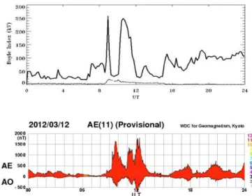
The Boyle index (Boyle et al., 1997), which is an asymp-totic polar cap potential, is calculated from the solar wind pa-rameters. The upper panel in Fig. 3 shows time series of the Boyle index provided from Rice Space Institute/Rice Univer-sity (http://mms.rice.edu/realtime/forecast.html). Large en-hancements are seen at around 09:00 and 11:00 UT in associ-ation with the solar wind variassoci-ation, suggesting the large polar
Figure 3.The upper panel indicates the Boyle index, which is an asymptotic polar cap potential (kV), on 12 March 2012 calculated from the solar wind parameters. The solar wind dynamic pressure (in units of nPa) is also shown with dotted line in the upper panel. The lower panel indicates the provisional geomagnetic field indices (AE and AO) on 12 March 2012. The number of stations used to derive the indices is shown in color.
cap potential drops after the periods. Note that the Boyle index could be a good predictor of the polar cap potential drop when the solar wind is steady and the index is less than 160 kV. The peak values exceeding 160 kV in Fig. 3 could be overestimated. The Boyle index is one of proxies for de-scribing the magnetospheric activity as a result of solar wind variations.
The solar wind–magnetosphere interaction during the pe-riod also caused changes in geomagnetic activity. As the ef-fects of the CME continued, periods of major storms were observed with isolated severe storm levels at high latitudes from 09:00–15:00 UT as shown in the provisional AE index (lower panel in Fig. 3).
3 ESR/EISCAT UHF radar observations
graphic meridional plane (yellow arrows in the right panel) and had a beam departing 30◦azimuthally from the meridional plane (red arrow in the right panel).
line-of-sight ion velocity data obtained from beam 1, beam 2, and beam 4 observations, we derive the ion velocity vector and then the electric field with the assumption of the spa-tial homogeneity of the beam areas as well as the temporal stability for the necessary time for scanning the three posi-tions (i.e., 8 min). The EISCAT UHF radar observaposi-tions were made during 07:00–13:00 UT on 12 March 2012.
The EISCAT Svalbard radar (ESR) at Longyearbyen is lo-cated at 78.2◦N, 16.0◦E (75.1◦N, 113.0◦E in geomagnetic coordinates). The LST and MLT at Longyearbyen are ap-proximately UT + 1 and UT + 3, respectively. Since we had limitations for the ESR operation because of a system prob-lem during the period, the ESR experiment was conducted in so-called CP3 mode with the 32 m antenna (magnetic meridian scanning with 15 beams with a time of 6 s in each beam) and field aligned direction observations were made with the 42 m antenna. The ESR observations were made during 07:00–12:00 UT. Figure 4 shows a schematic illustra-tion of the beam direcillustra-tions of the ESR and the EISCAT UHF radar employed in our observations.
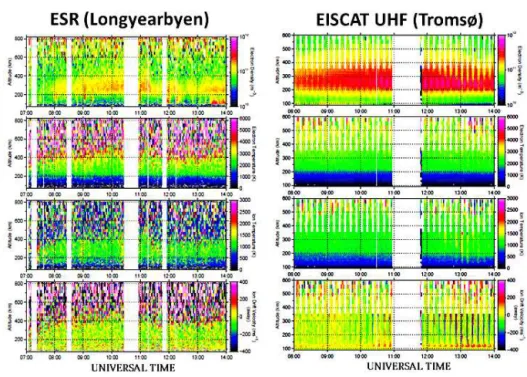
Figure 5 shows temporal variations of the electron density, electron temperature, ion temperature, and ion line-of-sight velocity (the ion motion away from the observation site is positive) from the top to the bottom, respectively. The left and right panels indicate values obtained from the ESR ob-servations with the 42 m antenna (in the altitude range of 90– 800 km) and the EISCAT UHF radar observations (in the alti-tude range of 90–600 km), respectively. Note that the results of all the beam directions are plotted every two minutes in the right panel. The ion temperature enhancements start at around 09:00 UT in the ESR observations, while variations are not so significant in other parameters and the EISCAT UHF radar observations at around 09:00 UT. During about 09:15–09:40 UT, large enhancements of the ion temperature
about 30 min (about 200–450 km altitude) while the electron temperature and ion velocity seem to vary with periods less than 10 min (about 300–450 km altitude). On the other hand, the EISCAT UHF radar did not observe significant changes in the ionospheric parameters during 10:00–11:00 UT. After 11:00 UT, the ionospheric parameters obtained from the EIS-CAT UHF radar observations show quite large variations, particularly seen in the ion temperature and velocity. The ESR, however, did not observe significant ionospheric varia-tions compared to the EISCAT UHF radar observavaria-tions after 11:00 UT although there are data gaps during about 11:20– 11:30 UT.
We made the same observations on 13 March. The val-ues of indices F10.7 and Kp were 141 sfu and 1 +∼2,
re-spectively, during the observational period on 13 March. The ionospheric parameters on 13 March obtained from the ESR and the EISCAT UHF radar are shown in Fig. 6 as a reference of the relatively quiet day. Although there are some data gaps because of the radar system problems, we can see the rela-tively quiet ionosphere with small variations. For example, the ion temperature at about 300 km obtained from the ESR and the EISCAT UHF radar varied from about 1000–1500 K except for some enhancements of about 2000 K.
Figure 5.Ionospheric variations in the altitude range of 90–800 km observed with the EISCAT Svalbard 42 m radar (ESR) at Longyearbyen (left) and those in the altitude range of 90–600 km observed with the EISCAT UHF radar at Tromsø (right) on 12 March. The electron density, electron temperature, ion temperature, and ion drift velocity are shown from the top to bottom, respectively, in each panel.
ion temperature were generated at higher latitudes; namely, variations of Ti-1 were significant during the period. After about 11:00 UT, the heating regions seem to move to lower latitudes; in particular, enhancements of Ti-2 and Ti-5 are re-markable. The maximum value of Ti-5 is about 3800 K at around 12:00 UT.
The electric field is obtained from the EISCAT UHF radar ion drift observations at 282 km altitude with beam 1, beam 2, and beam 4. Figure 8 shows the electric field varia-tions on March 12 for geographically northward (blue line) and eastward (red line) components. At around 09:30 UT, small enhancements are seen in the eastward component. At around 11:10 and 12:00 UT, large enhancements are seen in the northward component. The values of the northward com-ponent of the electric field at around 11:10 and 12:00 UT are about 85 and 126 mV m−1, respectively. These variations are almost consistent with those of the ion temperature (2, Ti-3, Ti-4, and Ti-5). In particular, the electric field variations after 11:00 UT are well in agreement with Ti-5.
Figure 9 shows ESR observations on 12 March with the 32 m antenna which scanned geomagnetic meridional di-rections. The left panel indicates ionospheric variations ob-served from the northward-directed beam with elevation an-gles 32–52◦. The right panel is the same as the left one except for the southward-directed beam. Note that the ion drift di-rection away from the observation site is positive; namely, the poleward ion motion is positive and negative in the left and right panels, respectively. The ion temperature in the altitude range of about 120–300 km is much larger in the
northern direction (left panel) than that in the southern di-rection (right panel) before about 09:30 UT.
The northward observation data (left panel in Fig. 9) show enhancements of the ion temperature in the altitude range of about 120–250 km at 09:18 UT. After that, large enhance-ments of the ion temperature (> 3000 K) above about 100 km altitude are seen at 09:28 UT. The large equatorward ion mo-tion (negative values) above about 150 km altitude is also seen at 09:28 UT. The poleward and equatorward ion motions are seen alternately until 12:00 UT. The enhancements of the ion temperature seem to have occurred during the equa-torward ion motion. The southward observation data (right panel in Fig. 9) shows enhancements of the ion temperature (> 3000 K) above about 100 km altitude just after 09:30 UT. At that time, strong poleward ion motion (negative values) is seen. The ion temperature decreased to about 1000–2000 K during about 10:00–11:00 UT. The ion temperature increased again at around 11:00–11:20 UT. After about 11:30 UT, the ion temperature gradually decreased again. The variations of the ion temperature and motion are almost consistent with the northward observations with the EISCAT UHF radar (in particular, beam 2) at Tromsø.
4 Summary and discussion
Figure 6.Same as Fig. 5 except for 13 March; observations on the relatively quiet day.
Figure 7. Ion temperature variations at about 300 km altitude on 12 March. The black line indicates the ion temperature observed with ESR 42 m at Longyearbyen. The red, blue, and green lines show the ion temperatures derived from the EISCAT UHF radar observations at Tromsø with beam 2, beam 3, and beam 4, respec-tively. The red dotted line shows the ion temperature derived from the EISCAT UHF observations at Tromsø with beam 1.
successfully observed variations of the polar ionosphere due to shock downstream structure of the solar wind which was caused by the arrival of a CME associated with the M8.4 solar flare event on 10 March. The characteristics of the changes in the solar wind were (1) passage of interplanetary shock structures, e.g., sudden excursions of the solar wind speed (from∼420 to∼580 km s−1) and density (from∼10
to ∼40 particles/cc on average), and short-duration
south-ward turning of the IMF-Bz component and (2) southward
IMF-Bzcomponent lasting more than 1.5 h after the passage
of the interplanetary shock.
Figure 8.Electric field variations obtained from the EISCAT UHF radar ion drift observations at 282 km altitude with beam 1, beam 2, and beam 4 on 12 March. The geographically northward and east-ward components are shown with blue and red lines, respectively.
Before the arrival of the interplanetary shock, the ion tem-perature at the higher latitude (see the left panel in Fig. 9) in the polar cap region is much larger (by more than 1000 K) than that at the lower latitude (see the right panel in Fig. 9). Some previous studies reported high ion temperature and/or large heating rate in the polar cap region (e.g., Fujiwara et al., 2007, 2012). The present observations are consistent with the previous results of the “hot polar cap”.
Figure 9.ESR observations with the 32 m antenna on 12 March. The left panel indicates ionospheric data obtained from the northward-directed beams with elevation angles 32–52◦. The right panel is the same as the left one except for southward-directed beams. Note that the ion drift direction away from the observation site is positive; namely, the poleward ion motion is positive and negative in the left and right panels, respectively.
culated to be 88, 257, and 114 kV by using the ACE data at 08:46, 08:56, and 09:06 UT, respectively. In the second stage, there was strong heating in the lower latitude region (to the south of Longyearbyen and north of Tromsø) of the polar ionosphere, which was in association with the south-ward IMF-Bz component lasting more than 1.5 h after the
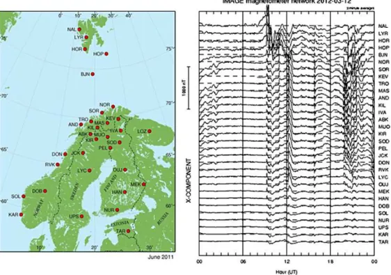
passage of the shock structures. The polar cap size seemed to have expanded. The polar cap potential also seemed to be large; the Boyle index was calculated to be more than 200 kV and 175–91 kV by using the ACE data during 10:26– 11:06 UT and 11:16–11:36 UT, respectively. Figure 10 shows the X-components of the geomagnetic field obtained from the IMAGE magnetometer network observations (http://www. ava.fmi.fi/image/). The IMAGE network covers the geo-graphic/geomagnetic latitude region from 78.92◦/75.25◦(Ny Ålesund: NAL) to 58.26◦/54.47◦(Tartu: TAR). The latitudi-nal variation of the geomagnetic field suggests the existence of strong currents at higher and lower latitudes in the first and second stages, respectively, as shown in Fig. 10. The spatiotemporal variations of the geomagnetic field are con-sistent with the ion temperature variations shown in Figs. 5, 7, and 9. The geomagnetic field variations obtained with the magnetometer could have been caused by the Hall currents, while the Pedersen currents are associated with Joule heat-ing. Since the Hall and Pedersen currents could be related, the magnetometer data should reflect variations of the heat-ing rate and the heatheat-ing region.
Many researchers have investigated variations of the ionosphere/thermosphere caused by solar wind high-speed streams/CIRs during the declining phase and near the min-imum of the solar cycle. For example, Gardner et al. (2012) showed the ion temperature enhancement due to arrival of the solar wind high-speed streams/CIRs from the ESR obser-vations during the period of days 194–201 in 2007. The ion temperature changed from about 820 to more than 1300 K (rise of about 500–600 K) within about two days. On the other hand, the ESR observed the ion temperature rise of about 2300 K within about 1.5 h in the present study, namely, during periods of the CME-induced geomagnetic activity. As mentioned by Chen et al. (2012), the ion temperature rise due
ionospheric/atmospheric disturbances (TIDs/TADs), will be investigated from general circulation model (GCM) simula-tions (e.g., Fujiwara and Miyoshi, 2006, 2009) as the next step of the present study.
Acknowledgements. We thank the staff of EISCAT for operating the facilities. EISCAT is an international association supported by re-search organizations in China (CRIRP), Finland (SA), Japan (NIPR and STEL), Norway (NFR), Sweden (VR), and the United King-dom (NERC). We thank the ACE SWEPAM instrument team and the ACE Science Center for providing the ACE data. Thanks also to the staff of WDC-C2 for providing the provisional geomagnetic indices. The solar image data obtained from the STEREO observa-tions were provided by the STEREO Science Center/NASA. We thank the institutes who maintain the IMAGE magnetometer ar-ray and RSI/Rice University who provided the Boyle index. This work was supported in part by Grant-in-Aid for Scientific Research B (22403010, 23340144, 23340149, 25287126) by the Ministry of Education, Science, Sports and Culture, Japan. A part of this work was also supported by the joint research programs of the Solar-Terrestrial Environment Laboratory, Nagoya University and the Na-tional Institute of Polar Research, Japan.
Topical Editor K. Hosokawa thanks M. Kosch and one anony-mous referee for their help in evaluating this paper.
References
Boyle, C. B., Reiff, P. H., and Hairston, M. R.: Empiri-cal polar cap potentials, J. Geophys. Res., 102, 111–125, doi:10.1029/96JA01742, 1997.
Carlson, H. C., Spain, T., Aruliah, A., Skjaeveland, A., and Moen, J.: First-principles physics of cusp/polar cap ther-mospheric disturbances, Geophys. Res. Lett., 39, L19103, doi:10.1029/2012GL053034, 2012.
ICME-and CIR-dominated solar wind, J. Geophys. Res., 111, A07S07, doi:10.1029/2005JA011436, 2006.
Fujiwara, H. and Miyoshi, Y.: Characteristics of the large-scale traveling atmospheric disturbances during geomagnetically quiet and disturbed periods simulated by a whole atmosphere general circulation model, Geophys. Res. Lett., 33, L20108, doi:10.1029/2006GL027103, 2006.
Fujiwara, H. and Miyoshi, Y.: Global structure of large-scale dis-turbances in the thermosphere produced by effects from the up-per and lower regions: simulations by a whole atmosphere GCM, Earth Planets Space, 61, 463–470, 2009.
Fujiwara, H., Kataoka, R., Suzuki, M., Maeda, S., Nozawa, S., Hosokawa, K., Fukunishi, H., Sato, N., and Lester, M.: Elec-tromagnetic energy deposition rate in the polar upper thermo-sphere derived from the EISCAT Svalbard radar and CUT-LASS Finland radar observations, Ann. Geophys., 25, 2393– 2403, doi:10.5194/angeo-25-2393-2007, 2007.
Fujiwara, H., Nozawa, S., Maeda, S., Ogawa, Y., Miyoshi, Y., Jin, H., Shinagawa, H., and Terada, K.: Polar cap ionosphere and thermosphere during the solar minimum period: EISCAT Sval-bard radar observations and GCM simulations, Earth Planets Space, 64, 459–465, 2012.
Gardner, L., Sojka, J. J., Schunk, R. W., and Heelis, R.: Changes in thermospheric temperature induced by high-speed solar wind streams, J. Geophys. Res., 117, A12303, doi:10.1029/2012JA017892, 2012.
Kataoka, R. and Miyoshi, Y.: Flux enhancement of radiation belt electrons during geomagnetic storms driven by coronal mass ejections and corotating interaction regions, Space Weather, 4, S09004, doi:10.1029/2005SW000211, 2006.
Kataoka, R., Watari, S., Shimada, N., Shimazu, H., and Marubashi, K.: Downstream structures of interplanetary fast shocks asso-ciated with coronal mass ejections, Geophys. Res. Lett., 32, L12103, doi:10.1029/2005GL022777, 2005.
Lei, J., Thayer, J. P., Forbes, J. M., Sutton, E. K., and Nerem, R. S.: Rotating solar coronal holes and periodic modulation of the upper atmosphere, Geophys. Res. Lett., 35, L10109, doi:10.1029/2008GL033875, 2008a.
Lei, J., Thayer, J. P., Forbes, J. M., Wu, Q., She, C., Wan, W., and Wang, W.: Ionosphere response to solar wind high-speed streams, Geophys. Res. Lett., 35, L19105, doi:10.1029/2008GL035208, 2008b.
Lei, J., Thayer, J. P., Wang, W., and McPherron, R. L.: Im-pact of CIR storms on thermosphere density variability dur-ing the solar minimum of 2008, Solar Phys., 274, 427–437, doi:10.1007/s11207-010-9563-y, 2011.
Liu, H., Lühr, H., Henize, V., and Köhler, W.: Global distribution of the thermospheric total mass density derived from CHAMP, J. Geophys. Res., 110, A04301, doi:10.1029/2004JA010741, 2005. Lühr, H., Rother, M., Köhler, W., Ritter, P., and Grunwaldt, L.: Thermospheric up-welling in the cusp region: Evidence from CHAMP observations, Geophys. Res. Lett., 31, L06805, doi:10.1029/2003GL019314, 2004.
Richardson, I. G., Webb, D. F., Zhang, J., Berdichevsky, D. B., Biesecker, D. A., Kasper, J. C., Kataoka, R., Steinberg, J. T., Thompson, B. J., Wu, C.-C., and Zhukov, A. N.: Major magnetic storms (Dst≤ −100 nT) generated by coro-tating interaction regions, J. Geophys. Res., 111, A07S09, doi:10.1029/2005JA011476, 2006.
Thayer, J. P., Lei, J., Forbes, J. M., Sutton, E. K., and Nerem, R. S.: Thermospheric density oscillations due to periodic so-lar wind high-speed streams, J. Geophys. Res., 113, A06307, doi:10.1029/2008JA013190, 2008.