A Graph Calculus for Predicate Logic

D. Kesner and P. Viana (Eds.): LSFA 2012

EPTCS 113, 2013, pp. 153–168, doi:10.4204/EPTCS.113.15

c

Veloso & Veloso

This work is licensed under the Creative Commons Attribution License. Paulo A. S. Veloso

COPPE-UFRJ

Systems and Computer Engin. Program UFRJ: Federal University of Rio de Janeiro

RJ, Brazil pasveloso@gmail.com

Sheila R. M. Veloso FEN-UERJ

Systems and Computer Engin. Dept., Fac. of Engineering UERJ: State University of Rio de Janeiro

RJ , Brazil

sheila.murgel.bridge@gmail.com

We introduce a refutation graph calculus for classical first-order predicate logic, which is an exten-sion of previous ones for binary relations. One reduces logical consequence to establishing that a constructed graph has empty extension, i. e. it represents⊥. Our calculus establishes that a graph has empty extension by converting it to a normal form, which is expanded to other graphs until we can recognize conflicting situations (equivalent to a formula and its negation).

1

Introduction

We present a refutation graph calculus for classical first-order predicate logic. This approach is based on reducing logical consequence to showing that a constructed graph has empty extension, representing the logical constant⊥. Our sound and complete calculus establishes when a graph has empty extension.

For instance, given formulasψ,θandϕ, to establish thatϕfollows from{ψ,θ}, we construct a graph G_{corresponding to{ψ,θ} ∪ {¬ϕ}and show that}G_{has empty extension. Now, our calculus establishes}

that a graph has empty extension by converting it to a normal form, which is expanded to other graphs until we can recognize conflicting situations (equivalent to a formula and its negation).

Formulas are often written down on a single line [3]. Graph calculi rely on two-dimensional repre-sentations providing better visualization [2].1 In the realm of binary relations, a simple calculus (with linear derivations) [2, 3] was extended for handling complement: direct calculi [5, 7] and refutation cal-culi [13]. Our new calculus is a further extension, inheriting much of the earlier terminology (such as ‘graph’, ‘slice’ and ‘arc’), together with some ideas from Peirce’s diagrams for relations [11, 4]. The present calculus involves two new aspects: extension to arbitrary predicates (which affects the represen-tation) and allowing formulas within the graphs.

The structure of this paper is as follows. Section 2 motivates the underlying ideas with some illus-trative examples. Section 3 introduces our graph language: syntax, semantics and some constructions. In Section 4 we introduce our graph calculus: its rules and goal. Section 5 presents some concluding remarks, including comparison with related works.

2

Motivation

We begin by motivating our ideas with some illustrative examples.

∗_{Research partly sponsored by the Brazilian agencies CNPq and FAPERJ.} 1_{The structure of(x+y)·(z÷w)is more apparent in the notation}



 x

+

y  ·



 z ÷ w



We know that consequence can be reduced to unsatisfiability. We will indicate how one can represent formulas graphically and then establish consequence by graphical means.

First, we indicate how we can represent (some) formulas graphically (see 3.1 for more details). We represent an atomic formula by arrows to predicate symbols coming from its arguments. So, we represent the formulas p(u)and r(u,v), respectively, as follows:

p

O

O

u

r

u

D

D

v

Z

Z

The former illustrates a 1-ary arc. The latter is an example of a 2-ary arc, which will be satisfied by the choices of valuesaandbfor u and v, respectively, with the pair(a,b)in the 2-ary relation interpreting r. We obtain a representation for a conjunction by joining those of its formulas. So, we represent the formula p(u)∧r(u,v)as follows:

p

[

[ r

u

C

C

v

[

[

This set of 2 arcs is an example of a draft, which also represents the set{p(u),r(u,v)}. This draftD_will be satisfied exactly by the assignments satisfying both p(u)and r(u,v).

To represent an existential quantification, we hide the node corresponding to the quantified variable, leaving only the rest visible. For instance, from formula p(u)∧r(u,v), we obtain∃x(p(x)∧r(x,v)). We can use the representation of the former to represent the latter: we place the above draftD_{within a box} and mark v as visible, which we represent as follows:

p

Z

Z r

u

E

E

~v

Y

Y

This is an example of a 1-ary slice. The interpretation of this sliceS_{is the 1-ary relation consisting of} the valuesbsuch that, for somea, the assignment u7→a, v7→bsatisfies the underlying draftD_.

Now, we can represent formula¬∃x(p(x)∧r(x,v))by complementing this sliceS_{. As stands for} complement, we represent¬∃x(p(x)∧r(x,v))as follows:

p

Z

Z r

u

E

E

~v

Y

Y

A draft consists of finite sets of names and of arcs (giving constraints on the names). A slice consists of a draft and a list of distinguished names, which we indicate by special marks, such as ‘→’.

Next, we illustrate how one can establish consequence by graphical means. The idea is reducing unsatisfiability of a (finite) set of formulas to that of its corresponding draft.

We begin with an example that is basically propositional. Then, we examine other examples with equality=. and existential quantifiers (see 3.2 and 4.1 for more details).

p(u) q(u) p(u)∧q(u) ¬p(u) p \ \ u q O O u p \

\ qOO

u

p

B

B

u

We can obtain a representation for the set{p(u)∧q(u),¬p(u)}by joining those of its formulas:

p

\

\ qOO BBp

u

Within this draft for{p(u)∧q(u),¬p(u)}, we find the conflicting situation (as stands for complement):

p

\

\ BBp

u

Thus, the representation of{p(u)∧q(u),¬p(u)}is unsatisfiable.

Example 2.2. We know thatp(u)6|=p(v), i. e.{p(u),¬p(v)} 6|=⊥. The corresponding draft is:

p

O

O pOO

u v

Here, we do not find conflicting arcs.2 In fact, we can read from the representation a modelM_=hM,pM_i, with M:={u,v}andpM:={u}, where one can satisfyp(u)and¬p(v).

Example 2.3. We reducep(v)∧v=. u|=p(u)to the unsatisfiability of the set{p(v)∧v=. u,¬p(u)}. We have the graphical representations as sets of arcs as follows:

p(v)∧v=. u ¬p(u) {p(v)∧v=. u,¬p(u)}

p Z Z . = C

C [[

v u p C C u p Z Z . = C

C [[ _DDp

v u

Now, we can simplify the representation of{p(v)∧v=. u,¬p(u)}, by renamingvtou:

p Z Z . = C

C [[ _DDp

v u

transforms to

p

]

] AAp

u

This final representation is not satisfiable (cf. Example 2.1).

Example 2.4. We reducer(u,v)|=∃zr(u,z)to{r(u,v),¬∃zr(u,z)} |=⊥. As before, we can represent formular(u,v)by the single-arc draft:

2_{Indeed, we have:} p

O O u but not p O O u

r

u

C

C

v

[

[

Also, we can represent¬∃zr(u,z)by the following1-ary arc:

u

~u

r v

Thus, we can represent{r(u,v),¬∃zr(u,z)}by the draft:

r

v

_

_

u

~u

r v

?

?

Now, with~u7→u,v7→v, we have a copy of the slice under complement within the draft, namely:

slice → draft

~u r

v

D

DYY

u r

v

=

=__

So, the representation of{r(u,v),¬∃zr(u,z)}is not satisfiable.

Example 2.5. We reduce∃x∃y[r(u,x)∧s(x,y)]|=∃zr(u,z)to{∃x∃y[r(u,x)∧s(x,y)],¬∃zr(u,z)} |=⊥. Proceeding as before, we can be represent{∃z∃y[r(x,z)∧s(z,y)],¬∃zr(u,z)}as:

~u r

v s

w

E

EYY EE VV

8

8

u

~u

r v

u r

v s

w

~u

r v

E

EYY EEVV

3

Graph Language

We now introduce our concepts: expressions, slices and graphs will give relations, whereas arcs, sketches and drafts will correspond to constraints. We will examine syntax and semantics (in 3.1) and then some concepts and constructions (in 3.2).

We first introduce some notations. Given a function f :A→B, we use f(a)oraf for itsvalueat an elementa∈A; which we extend to lists and sets. For a lista=ha1, . . . ,aki ∈Ak, we use f(a)oraf for thelist of valuesha1f, . . . ,akfi ∈Bk; for a setN, we use f(N)orNf for theset of values{af :a∈N}. Given a lista=ha1, . . . ,aki ∈Ak, we employafor itsset of components. The null listisλ:=h i. We sometimes write a listha1, . . . ,akisimply asa1. . .ak.

We will use names (or parameters) for marking free places and variables for marking bound places, as usual in Proof Theory [12]. To quantify a formulaϕ we replace a name u by a new variable (not appearing inϕ) obtaining∃xϕ[u/x]and∀xϕ[u/x]. Also, given lists u, ofndistinct names, andx, ofn

distinct variables not occurring inϕ, we have the formulas∃n_{xϕ[u/x]and∀}n_xϕ[u/x].

We will consider first-order predicate languages (without function symbols, except the constant⊥), each one characterized by pairwise disjoint sets as follows:

(Nm_{) an infinite linearly orderedset of names}Nm_;

(Vr) a denumerably infiniteset of variablesVr_;

(Pr_{) (possibly empty, but pairwise disjoint) sets}Pr_{nofn-arypredicate symbols, forn∈IN.}

Givenm∈IN+, we use umfor themth name. Givenn∈IN, we use un:=hu1, . . .unifor thelist of the

first n names(with u0=λ). Also, given a setv⊆Nm_{of names, we use~vfor the list of the names in v in} the ordering ofNm_{. For a formulaϕ, we useNF[ϕ]for theset of names occurring inϕ.}

3.1 Syntax and semantics

We now introduce the syntax and semantics of our concepts. We first examine the syntax of our concepts. The objects of our graph language are defined by mutual recursion as follows.

(E) Ann-aryexpressionis ann-ary predicate symbol, a formula withnnames, ann-ary slice or graph (see below), or E, where E is ann-ary expression. For instance,⊥is a 0-ary expression,=. and=.

are 2-ary expressions, whereas p(u)and p (for p∈Pr_{1) are 1-ary expressions.}

(a) Anm-aryarca_{over set}N_⊆Nm_{of names is a pair E/v (also noted}E

v), where E is anm-ary expression and v∈Nm_{. Examples are⊥/λ,=}._{/u v, p/u, q(u)/v (for p,q∈Pr}

1) and s/u w (for s∈Pr2).

(D) AdraftD_=hN_,A_{i is a sketch with finite sets}N_{of names and}A_{of arcs. An example of draft is} D′_=h{u,u′_,v,w,w′_{},{p/u,q(u)/v,=}._{/w w}′_{,s/u w}i.}

(S) Ann-arysliceS_=hS_{: ˆ}s_{iconsists of itsunderlying draft}S_:=hN_,A_{iand adistinguished list}s_{ˆ, with} ˆ

s_∈Nn_{. For instance,}S_=h{u,u′_,v,w,w′_{},{p/u,q(u)/v,=}._{/w w}′_{,s/u w}: u v viis a 3-ary slice with} underlying draftS₌D′_{(as above) and distinguished list ˆ}s_=hu,v,vi.

(G_{) Ann-arygraphis a finite set ofn-ary slices.}

In particular, the empty graph{ }has no slice. Example 4.5 (in 4.2) will show a 2-slice graph.

Note that expressions, arcs, slices and graphs are finite objects, whereas sketches are not necessarily so. Sketches will be useful for representing models and constructing co-limits. Also, some concepts and results do not depend on finiteness (see 3.2), which will be important in Section 4. We wish to represent these finite objects graphically by drawings (cf. the examples in Section 2). For this purpose, we employ two sorts of nodes: name nodes (labeled by names) and expression nodes (labeled by expressions). Some representations aiming at precision and readability are as follows.

We represent anm-ary arc E/v, with v=hv1, . . . ,vmi, bymarrows connecting each node labeled by

vi to the node labeled by E. For instance, we can draw a 3-ary arc t/hu,v,wi as

t ր ↑ տ

u v w

.

To clarify (as in t

u v u), we may use distinct kinds of lines or label them by numbers.

3 _{A more compact}

version uses is v1 →r v2 for the 2-arc r/v1v2, representing 1-ary, 3-ary and 4-ary arcs, respectively, as:

p

v1

, v1 t //v3

v2

O

O and v1

q

/

/v4

v2 //

O

O

v3

.

We can indicate the components of a distinguished list by marking their nodes, say with numbers, e. g.hu,v,uiby u1,3v2. Also, it may be convenient (for easier visualization) to enclose a sliceS_{within a full}

box, S _{, and a graph}G_{within a dashed box,} G _{. For instance, Example 2.5 (in Section 2) shows a 0-ary} sliceS_=h{u,v,w},A_{:λi, with}A_{={r/u v,s/v w,}T_{/u}, where}T_{is the 1-ary sliceh{u,v},{r/u v}: ui.}

Given a list w of names, thearclesswsliceis the slice⊤w:=hw,/0: wi. Thearcless m-ary sliceis

the slice⊤m:=⊤um(umis the list of the firstmnames) and them-node arcless draftis⊤_m=hum,/0i. The arc of formulaϕ, with set v of names, isa_{[ϕ]:=ϕ/~v. (The arc of a sentenceτis 0-ary:}a_{[τ] =τ/λ, which} we represent as the expression node τ.) The sketch of the set of arcsA_{is the sketch} Sk_[A_]:=hN_,A_i, whereN_{consists of the names occurring in the arcs of} A_: N_:=S_{w⊆Nm_{: E/w∈}A_{}. For instance,} Sk_{[{s/u v,p(v)/w}] =h{u,v,w},{s/u v,p(v)/w}i.}

We may wish to add an arca_{=E/v to a sketch, a slice or a graph. For a sketch Σ=h}N_,A_{i, we} setΣ+a_:=hN_∪v,A_{∪ {}a_{}i; for a slice}S_=hS_{: ˆ}s_{i, we set}S₊a_:=hS₊a_{: ˆ}s_{i; for a graph}G_{, we set} G₊a_:={S₊a _:S_∈G_{}. Thedifference sliceof a finite set of arcs}A_{with respect to an arc}a_{=E/v is}

the 0-ary sliceDS_[A∠a_]:=hSk_[A_{] +E/v :λi. For instance, Example 2.3 (in Section 2) represents the} set{p(v)∧v=. u,¬p(u)}by the difference sliceDS_[{p/v,=._{/v u}}∠_{p/u]. We will give some intuition for} using 0-ary slices in 3.2.

We now examine the semantics of our concepts and related ideas.

AmodelM_{has as its universe a setM6=/0and realizes each n-ary predicate symbol p∈}Pr_{nas an}

n-ary relation pM⊆Mn(with=.M:={ha,ai ∈M2 :a∈M}). AnM-assignmentfor setN_⊆Nm_{of names} is a functiong:N_{→M. A formulaϕwith setvofnnamesdefinesthen-ary relationϕ}M

⊆Mnconsisting

of the values of its ordered names for the assignments satisfyingϕ:ϕM_:={~vh_∈Mn _{:M|=ϕ[[h]]}. For} instance, for 2-ary predicate symbol r, r(u1,u2)M=rM, r(u2,u1)M={hb,ai ∈M2 :ha,bi ∈rM} and

r(u1,u1)M={hai ∈M1 :ha,ai ∈rM}. Also,⊥M:=/0.

We now introduce the meanings of the concepts, again by mutual recursion.

(E) We define therelationof an expression as follows. For a predicate symbol p we have its relation:

[p]M:=p M

; for formula ϕ we have its defined relation: [ϕ]M:=ϕ M

; for a sliceS _{or graph}G_, we use the extensions: [S_]

M:= [[S]]M and[G]M:= [[G]]M(see below); for E, where E is ann-ary

expression, we use the complement:[E]M:=Mn\[E]M.

(a_{) An M-assignment g:}N_{→M satisfiesanm-ary arc E/v over}N_inM_(notedgME/v) iff v∈Nm

and vg_∈[E]

M. For instance,gM=./u v iff ug=vgandgMp/w iff wg∈[p]M=p M

.

(Σ) An assignmentgsatisfiesa sketchΣ=hN_,A_iinM_{(notedg:Σ→}M_{) iffgsatisfies every arc}a_∈A_.

(S) Theextensionof a slice is the relation consisting of values of its distinguished list for the assignments satisfying its underlying draft; for ann-ary sliceS_=hS_{: ˆ}s_i,[[S_]]M:={ˆsg_∈Mn _:g:S→M}.

(G) Theextensionof a graph is the union of those of its slices: [[G_]]M:=S_S∈G[[S_]]M.

Clearly,gME/v iffg6ME/v. Also, the arclessm-ary slice⊤mhas extension[[⊤m]]M=Mm.

An expression E isnulliff[E]M=/0in every modelM. For instance, the empty graph{ }is null.

Given a sketchΣ=hN_,A_{i and an arc}a_{=E/v, we say that}a_{is a consequence of Σ(notedΣ|=}a₎ iff, for every model M _{and M-assignment g:}N_{∪v→M, gsatisfies} a _{whenever g satisfiesΣ. Call} expressions E and Fequivalent (noted E≡F) iff, for every modelM_{,[E]M= [F]M. A slice} S_{and the} singleton graph{S_{}are equivalent (so they may be identified).}

We can reduce consequence to the difference slice: an arca _{is a consequence of a draft}D _{iff the} difference sliceDS_[A∠a_{]is null. So, we can also reduce logical consequence to a difference slice.}4

Proposition 3.1. Given a finite set Ψ of formulas and a formula θ: Ψ|=θ iff the difference slice

DS_[{a_{[ψ]:ψ∈Ψ}}∠a_{[θ]]is null.}

Proof. By the preceding remark, sinceg_Ma_[ϕ]iffM_|=ϕ[[g]].

Section 4 will present a calculus for establishing that an expression is null.

3.2 Concepts and constructions

We now examine some concepts and constructions. We first introduce morphisms for comparing sketches.

Consider sketchesΣ′=hN′_,A′_iandΣ′′_=hN′′_,A′′_{i. A functionη:}N′′_→N′ _{is amorphismfromΣ}′′ toΣ′ (notedη:Σ′′99K_Σ′_{) iff it preserves arcs: for every arc E/v∈}A′′_{, we have E/v}η_∈A′_{. We use} Mor_[Σ′′_,Σ′_{]for theset of morphismsfromΣ}′′_toΣ′_.

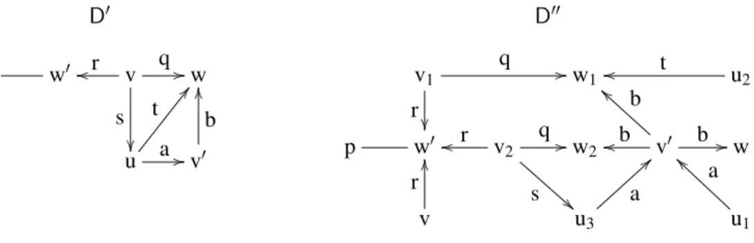
Example 3.1. Givenp∈Pr1andq,r,s,t,a,b∈Pr2, consider the draftsD′=hN′,A′iandD′′=hN′′,A′′i, with sets of nodesN′_={u,v,v′_,w,w′_}andN′′_{={u1,u2,u3,v,v1,v2,w,w1,w2,w}′_{}, and sets of arcs}

A′_{={q/v w,p/w}′_{,r/v w}′_{,s/v u,t/u w,a/u v}′_,b/v′_w}and

A′′_{={q/v1w1,q/v2w2,p/w}′_{,r/v w}′_,r/v1w′_,r/v2w′_{,s/v2u3,t/u2w1,a/u1v}′_,a/u3v′_,b/v′_w,b/v′_w1,b/v′_w2}.

These draftsD′_andD′′_{can be represented as in Figure 1. The mappingv}′_7→v′_;w′_7→w′_{;v,v1,v27→v;} w,w1,w27→wandu1,u2,u37→upreserves arcs.5 So, we have a morphismη:D′′99KD′. We also have formulasδ(D′_)andδ(D′′_{)such thatg:}D′_→M_iffM_|=δ(D′_{) [[g]]andg:}D′′_→M_iffM_|=δ(D′′_{) [[g]].}6

D′ D′′

p w′oo r v q //

s

w

u t

B

B

a _//v′

b

O

O v1

q

/

/

r

w1 oo t u2

p w′ oo r v2

q

/

/

s

!

!

w2 oo b v′

b

a

a

b _// w

v r

O

O

u3

a

>

>

u1

a

`

`

Figure 1: DraftsD′_andD′′_{(Example 3.1)}

A morphism transfers satisfying assignments by composition.

Lemma 3.1. Given a morphism η:Σ′′ 99K_Σ′_{, for every assignment g:}N_Σ′ →M satisfying Σ′, the compositeg·η:N_Σ′′→M is an assignment satisfyingΣ′′.

Proof. For every arc E/v∈A_Σ′′, we have E/vη∈A_Σ′, thus vg·η∈[E]_M, whenceg·ηME/v.

We now use morphisms to introduce zero sketches, slices and graphs.

A sketchΣ=hN_,A_{iiszeroiff there exist a slice}T_=hT_{: ˆ}t_{iand a morphismη:}T99K_{Σsuch that} T_/tˆη _{is an arc in} A_{. A slice}S_{iszero iff its underlying draft}S_{is a zero sketch. A graph iszero iff all}

its slices are zero slices. The sets of zero drafts, zero slices and zero graphs are all decidable, since, for draftsD′_andD′′_{, the set}Mor_[D′′_,D′_{]is finite.}

Example 3.2. Consider the following draftD_{and2-ary slice}T_:

D_=h{u′_,v′_,w′_},{r/u′_v′_,T_/u′_w′_,s/v′_w′_}i T_{=h{u,v,w},{r/u v,s/v w}: u wi}

u′ r //

T v′

s

w′

u1 r //v s

w2

The mappingu7→u′,v7→v′,w7→w′gives a morphismη:T99KD_{, with}ˆtη_=huη_,wη_i=hu′_,w′_{i. Thus,}

draftD_{is zero. So, slicesh}D_:λi,hD_{: u}′_i,hD_{: v}′_w′_iandhD_{: u}′_i,hD_{: u}′_v′_w′_{iare zero slices.}7

Lemma 3.2. No assignment can satisfy a zero sketch.

Proof. By Lemma 3.1,g:Σ→M_yieldsg·η:T_→M_{, thusgM}T_/ˆtη_whenceg6MT_/ˆtη_.

Corollary 3.1. Zero slices and zero graphs are null.

Proof. By Lemma 3.2: if[[S_{]]M6=/0, then some assignment satisfies}S_.

5_{For instance, for arc p/w ofD}′′_{, we have arc p/w}′_ofD′_{; for arcs q/v}

1w1and q/v2w2ofD′′, we have arc q/v w ofD′. 6_Takeδ(D′_{)as q(v,w)∧p(w}′_)∧r(v,w′_{)∧s(v,u)∧t(u,w)∧a(u,v}′_)∧b(v′_,w)andδ(D′′_{)as the conjunction of q(v}

1,w1),

We can now clarify the intuition behind using 0-ary difference slices (cf. 3.1). We know that a formula is satisfiable iff its existential closure is so. The latter will convert to a 0-ary (basic) graph, by Proposition 4.1 (in 4.1). Now, whether a slice is zero does not hinge on its distinguished list.

We now examine some categorical constructions: co-limits and pushouts [8].

The category of sketches and morphisms has co-limits. Given a diagram of sketchesΣi =hNi,Aii, itsco-limitcan be obtained as expected: obtain the co-limitN_{of the sets of names}N_{iand then transfer} arcs, by the functionsνi:Ni→N, i. e. A:=Si∈IAiνi. In particular, the pushout of drafts gives a draft.

We wish to glue a sliceT_{onto a draft or a slice via a designated list of names. This involves adding} the arcs ofT_{with its distinguished list identified to the designated list of names.}

Gluing can be introduced as an amalgamated sum (of drafts). Consider anm-ary sliceT_=hT_{: ˆ}t_i. Given a draftD_=hN_,A_{iand a list w∈}Nm_{ofmnames, theglued draftD}w_{Tis the pushout of the drafts}

D_{+w :=h}N_∪w,A_iandT_{over them-ary arcless draft⊤m=hu}m_{,/0iand the natural morphismsµ}′ _and µ′′(µ′: ui7→wiandµ′′: ui7→ˆti), as shown in Figure 2. Note thatν′(w) =ν′′(ˆt).

D_+w

ν′

&

&

hum_,/0i

µ′ 77

µ′′ ''

Dw_T

T ν′′

8

8

Figure 2: Pushout of drafts

Given ann-ary sliceS_=hS_{: ˆ}s_{i, we obtain theglued slice}SwT_{by transferring the distinguished list} ofS_{to the glued draft}SwT_:SwT_:=hSwT_:ν′_(ˆs_)i.8 _{We glue a graph by gluing its slices, i. e.}SwH_{is the} graph{Sw_{T:T∈H}. We glue onto a graph by gluing onto its slices, i. e.G}w_H:=S

S_∈GSwH.

Example 3.3. Consider the three slices: 1-ary S_=h{u,u′_,v′_{,v},{r/u u}′_,s/u′_v′_,t/v′_{v}: ui as well as} 2-aryT′_{=h{v,w},{a/w v}: w viand}T′′_{=h{w},{p/w,q/w}: w wi.}9 _{They are represented as follows:}

S T′ T′′

u1 r //u′ s //v′ t //v w1 a //v2 w1,2

p q

We obtain1-ary glued slices as follows:

Shu′,v′iT′_=h{u,u′_,v′_,v},

r/u u′,s/u′v′,t/v′v, a/u′v′

: ui Shu′,v′iT′′_=h

u,v, w

,

r/u w,s/w w,t/w v, p/w,q/w

: ui

u1 r _//u′ _v′ _v

s

#

#

a

;

;

t _{// u}1 r _//w

s

t _// v

p q

8_{A glued draft and slice are unique up to isomorphism. They can be made unique by a suitable choice of names. As} isomorphic objects have the same behavior, we often consider a sketch or a slice up to isomorphism.

Addition of a slice-arc is equivalent to gluing the slice. For instance, with the slices of Example 3.3: S₊T′_/u′_v′ _≡ Shu′,v′_i

T′_andS₊T′′_/u′_v′ _≡Shu′,v′_i

T′′_.

Proposition 3.2. Given a sliceS_{and an arc}T_/w: S₊T_{/w ≡}Sw_T.

Proof. By Lemma 3.1 and the pushout property .

It is not difficult to translate our graph language to the underlying first-order predicate language. It suffices to express the semantics of the graph language (in 3.1) by formulas.

4

Graph Calculus

We now introduce our graph calculus, with conversion and expansion rules. We employ R⋆ for the

reflexive-transitive closureof a binary relationRon a set, as usual.

Our conversion and expansion rules will transform an expression to an equivalent one. Thus, one can apply such a rule in any context. For instance, we will have a rule converting⊥to the empty graph{ }; so, we can apply it to convert⊥to{ }andS_+⊥/λtoS_{+{ }/λ, for any slice}S_{. Also, we can identify a} singleton graph with its slice (cf. 3.1): ifS⊲_{F then{}S_}⊲_{F and if E}⊲T_{then E}⊲_{T_}.

4.1 Conversion

We now introduce the basic objects and the conversion rules.

Thebasicobjects are defined (by mutual recursion) as follows. The basic expressions are the predi-cate symbols, other than=., andT_{, where}T_{is a basic slice (see below). An arc E/v is basic iff E is a basic} expression. A sketch is basic iff all its arcs are basic. A slice is basic iff its underlying draft is a basic sketch. A graph is basic iff its slices are all basic. For instance, the draftsD′ _andD′′_{, of Example 3.1,} andD_{, of Example 3.2, (in 3.2) are basic, whereas those in Examples 2.1, 2.2 and 2.3 are not basic.}

The conversion rules will transform an expression to an equivalent basic graph.

The formula rules will come from some equivalences between formulas and expressions We now illustrate some of these equivalences. For a 1-ary predicate p, formula p(v) is equivalent to the 1-ary slice h{v},{p/v}: vi, thus ¬p(v) is equivalent to the 1-ary expression p(v). Now, consider formu-las r(u,v) and s(v,w). For the conjunction r(u,v)∧s(v,w), we have a 3-ary sliceS _{equivalent to it,} namely the sliceS_=hN_,A_{: u v wi, with sets}N_={u,v,w}andA_{={r(u,v)/u v,s(v,w)/v w}. For the} disjunction r(u,v)∨s(v,w)we have a 3-ary graph G_{such that r(u,v)∨s(v,w)≡}G_{, namely the graph} G_{with 2 slices: h{u,v,w},{r(u,v)/u v}: u v wiandh{u,v,w},{s(v,w)/v w}: u v wi. Also, as the}

con-ditional formula r(u,v) →s(v,w) is logically equivalent to ¬r(u,v)∨s(v,w), it is equivalent to the 3-ary graph{h{u,v,w},{r(u,v)/u v}: u v wi,h{u,v,w},{s(v,w)/v w}: u v wi}. The existential formula ∃yt(u,y,w) is equivalent to the 2-ary slice h{u,v,w},{t(u,v,w)/u v w}: u wi. Also, as the universal formula∀yt(u,y,w) is logically equivalent to ¬∃y¬t(u,y,w), it is equivalent to the 2-ary expression h{u,v,w},{t(u,v,w)/u v w}: u wi.

Theformula rulesare the following 8 conversion rules eliminating formulas.

(α) For an atomic formula p(w): p(w)⊲_{hw,{p/w}: wi. So, we replace u=}. _{v, r(u,v)and t(u,v,v)by} .

=

@

@ ^^

u1 v2

r

A

A ]]

u1 v2

and

t

>

> QQ qq

(⊥) ⊥⊲_{{ }, i. e. we replace 0-ary formula⊥by the empty graph.}

(¬) ¬ϕ⊲_{ϕ. So, we replace¬(r(u,v)→s(v,w))by the 3-ary expression r(u,v)→s(v,w).} • Given formulasψandθ, withu:=NF[ψ]andv:=NF[θ], setw:=u∪v.

(∧) ψ∧θ⊲_{hw,{ψ/~u,θ/~v}:~wi. Thus, we can replace formula r(u,v)∧s(v,v)by the 2-ary slice} h{u,v},{r(u,v)/u v,s(v,v)/v}: u vi, which we can represent as:

r(u,v)

;

; dd 33s(v,vII )

u1 v2

(∨) ψ∨θ⊲_{{hw,{ψ/~u}:~wi,hw,{θ/~v}:~wi}. So, we can replace formula r(u,v)∨s(v,v) by the 2-ary} graph

h{u,v},{r(u,v)/u v}: u vi, h{u,v},s(v,v)/v}: u vi

.10

(→) ψ→ θ⊲_{hw,{ψ/~u,θ/~v} :~wi. So, we can replace formula p(u)→ r(v,w) by the 3-ary graph} {h{u,v,w},{p(u)/u}: u v wi,h{u,v,w},r(v,w)/v w}: u v wi}.

• Given a formulaϕand a setvof names, setu:=w\v, wherew:=NF[ϕ].

(∃∗_{) For formula∃}∗_xϕ[v/x],∃∗_{xϕ[v/x]⊲hw,{ϕ/~w}:~ui. Thus, we can replace ∃y∃zt(u,y,z)by the}

single-arc 1-ary sliceh{u,v,w},{t(u,v,w)/u v w}: ui, which we can represent as:

t(u,v,w)

;

; OO cc

u1 v w

(∀∗) For formula∀∗xϕ[v/x],∀∗xϕ[v/x]⊲_{hw,{ϕ/~w}:~ui. So, can we replace∀y∀zt(u,y,z)by the 1-ary} expressionh{u,v,w},{t(u,v,w)/u v w}: ui, which we can represent as:

t(u,v,w)

;

; OO cc

u1 v w

Example 4.1. Consider a formulaϕwith list of nameshu,v,wi, notedϕ(u,v,w). For the formula∃y∀zϕ(u,y,z), we have the conversions:

∃y∀zϕ(u,y,z) (∃ ∗₎

⊲ _h{u,v},{∀zϕ(u,v,z) u v }: ui

(∀∗₎

⊲ _h{u,v},{h{u,v,w},{ϕ/u v w}: u vi

u v }: ui

For the formula∀y∃zϕ(u,y,z), we have the conversions:

∀y∃zϕ(u,y,z)

(∀∗₎

⊲ _h{u,v},{∃zϕ(u,y,z) u v }: ui

(∃∗₎

⊲ _h{u,v},{h{u,v,w},{ϕ/u v w}: u vi

u v }: ui

10_{This graph can be represented as follows:}

u1 r(u,v) //v2

s(v,v)

1

1

K

K

By applying the 8 formula rules in any context, one can transform an expression to an equivalent expression without connectives or quantifiers.

Theequality ruleis the following conversion rule, eliminating expression=..

(=.) =. ⊲_{h{u},/0:hu,uii, where u∈}Nm_{. So, we can replace sliceh{u,v,w},{r/u v,=}._{/v w,s/u w}: v wi} by the sliceh{v,w},{r/u v,h{u},/0:hu,uii

v w ,s/u w}: v wi.

By using these 9 rules, one can eliminate logical symbols and predicates, but arcs whose expressions are slices or graphs, perhaps complemented, may appear. For instance, this happens with v=. w and ∃y(r(u,y)∧s(y,w)). The following rules will address these cases.

Thecomplementation rulesare the following 2 conversion rules, moving inside.

(∪) For ann-ary graphH_:H⊲_hw,{T_{/w :}T_∈H_{}: wi, where w is a list ofndistinct names. So, we can} replace the complemented 1-ary graph{S_,T_{}by the sliceh{v},{}S_/v,T_{/v}: vi.}

( ) E⊲_{E, i. e. eliminate double complementation.}

By applying these 2 complementation rules in any context, one can eliminate arcs whose expressions are complemented graphs.

Thestructural rulesare the following 3 conversion rules.

(−→∪ ) S₊H_/v⊲_{S₊T_{/v :} T_∈H_{}, i. e. replace addition of graph arc by alternative addition of its} slice arcs. So, we replace sliceS_+{T′_,T′′_{}/u by the graph{}S₊T′_/u,S₊T′′_/u}.

(→T) S₊T_/v⊲Sv_{T, i. e. replace addition of slice arc by glued slice.}

(↑) For ann-ary expression E: E⊲_{hw,{E/w}: wi, where w is a list ofndistinct names. So, for r∈}Pr_2, we can replace 2-ary expression r by the 2-ary sliceh{u1,u2},{r/u1u2}: u1u2i.

By means of rules (−→) and (∪ →), one can eliminate arcs whose expressions are graphs or slices.T

Rule (↑) converts expressions to slices and serves to eliminate p: p (⊲↑) _hun_,{p/un_{}: u}n_{i, for p∈}Pr_n.

Example 4.2. Consider the formular(v,w). We proceed much as in Example 4.1.

Formula∃y∀zr(y,z)converts to the0-ary sliceS_=h{v},{h{v,w},{r(v,w)/v w}: vi

v }:λi.

This sliceS_{is not basic, but it can be converted to a basic slice by (α) as follows:}

h{v},{

h{v,w},{r(v,w) v w }: vi

v }:λi

(α)

⊲ _h{v},{

h{v,w},{

h{v,w},{ r

v w}: v wi

v w }: vi

v }:λi

Formula∀y∃zr(y,z)converts to the0-ary expressionE=h{v},{h{v,w},{r(v,w)/v w}: vi

v }:λi.

This expressionEis not basic, but it can be converted to a basic expressionFby (α) as follows:

h{v},{h{v,w},{r(v,w)/v w}: vi

v }:λi

(α)

⊲ _h{v},{

h{v,w},{h{v,w},{ r

v w}: v wi/v w}: vi

v }:λi

Rule (→) gives some useful derived rules about arc addition, which we can use to shorten con-T versions (such shortenings were used in the examples of Section 2). We can replace addition of: a graph arc by gluing the graph ((−→):H S₊H_/v⊲⋆Sv_{H), a complemented-graph arc by addition of}

par-allel complemented-slice arcs (S₊H_/v⊲⋆S_+{T_{/v :} T_∈H_{}) and an equality arc by node renaming} (S₊₌._{/u v}⊲⋆S_[u/v],S₊₌._{/u v}⊲⋆S_[v/u]).

We can also replacenconjunctions and disjunctions by slices and graphs, respectively.11

Example 4.3. Consider the formulas(v′,w′)∧ ∃x[r(v′,x)∧ ¬∃y(r(x,y)∧s(y,w′))]. This expressionE

can be converted to the2-ary slicehD_{: v}′_w′_{i, where}D_{is the draft of Example 3.2 (in 3.2).}

We can convert expressions in a modular way.

Lemma 4.1. IfS⊲⋆G_andE⊲⋆H_{, then}S_+E/v⊲⋆GvH_.

Proof. By (−→) rule:H S_+E/v⊲⋆G₊H_/v={P₊H_{/v :} P_∈G_} ( H −→)

⊲ _{Pv_H:P∈G}=Gv_H.

Thus, one can obtain a basic form forS_{+E/v from basic forms}Sb _{and E}b_{, forSand E.}

Proposition 4.1. Every n-ary expressionEcan be effectively converted to a basic n-ary graphEb_.

Proof. By induction on the structure of expressions.

Example 4.4. Given the predicate symbols of Example 3.1 (in 3.2), consider the formulaψ:

q(v,w)∧ ∃z[p(z)∧r(v,z)∧ ∃x∃y∃y′(s(v,x)∧t(x,w)∧a(x,y)∧b(y,w))].

Consider also the formulaθ:=∃3_x

1x2x3∃y′∃2y1y2∃z′∃2z1,z2χ, whereχis as follows:

p(z′)∧s(v2,x3)∧t(x2,z1)∧ 



q(y1,z1)

∧ q(y2,z2)



∧





a(x1,v′)

∧ a(x2,v′)

 ∧      

r(v,z′)

∧ r(y1,z′)

∧ r(y2,z′)

      ∧      

b(y′,w)

∧ b(y′,z1)

∧ b(y′,z2)

      .

Now, form the difference sliceDS_[{a_[ψ]}∠a_{[θ]] =h{v,w},{ψ/v w,θ/v w :λ}i. Expressionsψandθcan}

be respectively converted to the2-ary slicesS_=hD′_:hv,wiiandT_=hD′′_{:hv,wii, where}D′_andD′′_are

the drafts of Example 3.1. Thus, we haveDS_[{a_[ψ]}∠a_[θ]]⊲⋆_h{v,w},{S_{/v w,}T_{/v w :λ}i. Now, we can}

see thath{v,w},{S_{/v w,}T_{/v w :λ}i}( T →)

⊲ _hS₊T_{/v w :λi.}12_HenceDS_[{a_[ψ]}∠a_[θ]]⊲⋆_hS₊T_{/v w :λi.}

4.2 Derivations

We now introduce the remaining rule and finish the presentation of our calculus.

First, let us review Examples 4.3 and 4.4 (in 4.1). Formula E of Example 4.3 converts to the 2-ary slicehD_{: v}′_w′_{i, which was seen to be zero in Example 3.2 (in 3.2). Thus, formula E is unsatisfiable. Now,} consider formulasψandθof Example 4.4, where we have seen thatDS_[{a_[ψ]}∠a_[θ]]⊲⋆_hS₊T_{/v w :λi.} Now, Example 3.1 (in 3.2) shows a morphismη:T99KS_{, with ˆ}tη_=hvη_,wη_i=hv,wi=ˆs_{. Thus, draft} S₊T_{/v w is zero, whence, slice}DS_[{a_[ψ]}∠a_{[θ]]is null. Therefore, we can conclude thatψ|=θ.}

11_{For instance, with 3 formulas, we have r(u,v)∧s(v,w)∧p(w)⊲}⋆_{h{u,v,w},{r(u,v)/u v,s(v,w)/v w,p(w)/w}: u v wiand}

r(u,v)∨s(v,w)∨p(w)⊲⋆{h{u,v,w},{r(u,v)/u v}: u v wi,h{u,v,w},s(v,w)/v w}: u v wi h{u,v,w},{p(w)/w}: u v wi}.). 12_{Indeed:h{v,w},{S/v w,T/v w :λ}i=h{v,w},{T/v w :λ}i+S/v w}(

T

→)

Example 4.5. To introduce expansion and its usefulness, consider the3-ary sliceS_:

u1

T₁

r _//w3

T₂

w′ t //u2

where T_{1 := u}1 _→r _w→s _v2 _{, T}

2 := u1 →s w →t v2 .

SliceS _{is not zero; but in any model} M_{, the pair(g(w),g(w}′_{))is either in [s]M or in [s]M. So,} S_is

equivalent to the2-ary graphG_={S_+,S_{−}, with slices}S_+andS_{−, respectively as follows:}

u1

u1 _→r _w→s _v2

r _{// w}3

T₂

s

~

~

w′

t //v

2

u1

T₁

r _{// w}3

u1→s w→t v2

s





w′

t //v

2

SlicesS_+andS_{−are both zero, so graph}G_{is zero. Thus,}S_{is a null slice.}

The expansion rule will replace a slice by a graph with 2 alternative slices.

(⊳) For anm-ary sliceT_{and v∈}N_Sm_:S⊳_{SvT_,S₊T_/v}.

Note that bothSv_{TandS+T/v are basic wheneverSandTare basic.}

Lemma 4.2. For a sliceS_{, an m-ary slice}T_andv∈Nmm_: S_{≡ {}Sv_T,S+T/v}.

Proof. By Proposition 3.2 (in 3.2),S₊T_{/v ≡}SvT_{, and clearly}S _{≡ {}S₊T_/v,S₊T_/v}.

Aderivationconsists of applications of the conversion rules and the expansion rule: ⊢:= (⊲_∪⊳₎⋆_. A derivation isnormal iff applications of conversion rules precede applications of the expansion rule: E⊲⋆G⊳⋆H_{. In practice, as we wish to derive a zero graph, we may erase slices already found to be zero.} Letϕbe the formula r(u,w)∧t(w′,v)∧ ¬∃x[r(u,x)∧s(x,v)]∧ ¬∃y[¬s(u,y)∧t(y,v)]. Expression E :=∃xϕ[w′/x]converts to the sliceS_{of Example 4.5, where it expands to the graph}G_{. We thus have} the normal derivation E⊲⋆S⊳G_{, with}G_{a zero graph. Hence, formulaϕis unsatisfiable.}

4.3 Soundness and completeness

We now examine soundness and completeness of our calculus.

Soundness is clear (as E≡F, whenever E⊢F): if E⊢ H_andH_{is zero, then E is null. We will show} that a converse holds for basic graphs (if Eb_{is null then E}b _{expands to a zero graph), and we will have}

completeness of normal derivations: if E is null, then E⊲⋆_Eb_⊳⋆_{H, for some zero graphH.}

Henceforth, all sketches, drafts, slices and graphs will be basic. We define the following families of slices: the family

Z

Z

Z

Z

Z

The following simple properties of these families will be useful.

Lemma 4.3. For every graphG_:G_⊆

Z

Z

Proof. (⇒) If, for eachS_∈G_,S⊳⋆H_SandH_S⊆

Z

∈GHS,G⊳⋆HandH⊆

Z

Lemma 4.4. For every graphG_:G_⊆

Z

Z

Proof. By Lemma 4.3, since

Z

Z

Z

Z

Z

Z

Z

Z

Corollary 4.1. ForS_∈

Z

Proof. By Lemma 4.4: if{SvT_,S₊T_{/v} ⊆}

Z

Z

We will show that a sliceS_∈

Z

Given a slice S_∈

Z

Z

whose underlying drafts are connected by morphismsµn fromSn to Sn+1, which we extend naturally

to morphismsµi_j :S_i99KS_{j, fori≤ j. Consider the co-limit of this draft diagram: sketchΣ=h}N_,A_i with morphismsνn:Sn99KΣ(cf. 3.2). We use this co-limit sketchΣto define anatural modelMwith

M:=N_{, and p}M

:={v∈Mn : p/v∈A_{}, for p∈}Pr_n.

By construction, the co-limit sketch Σis saturated in the following sense: given any m-ary slice T_=hT_{: ˆ}t_{iand w∈}Nm_{, we have arcT/w∈Aor there is a morphismη:T99KΣwith ˆt}η_=w.

We can establish that satisfying assignments are morphisms.

Lemma 4.5. Given a draftD_andg:N_D→M,g:D_→M_iffg:D99K_Σ.

Proof. By structural induction (on the total number of complemented slice arcs occurring inD_).

Finally, sinceν0:S99K_{Σ, we haveν0(}s_ˆ0)∈[[S_]]M6=/0. Therefore, ifG_6⊆

Z

Theorem 4.1. Consider an n-ary expressionE.

(⊢) IfE ⊢H_andH_{is zero, thenEis null.}

(⊲⋆_;⊳⋆) IfEis null, thenE⊲⋆_Eb_⊳⋆_{H, for some zero n-ary graphH.}

5

Conclusion

We now present some concluding remarks, including comparison with related works.

We have presented a refutation graph calculus for classical first-order predicate logic. This sound and complete calculus reduces logical consequence to establishing that a constructed graph is null, i. e. has empty extension in every model. Our calculus uses formulas directly and can represent them by arcs. We have a simple strategy for establishing that a graphG_{is null: first convert}G_{to basic form, then} apply repeatedly the expansion rule, erasing slices found to be zero, which is decidable (cf. 3.2), trying to obtain the empty graph. Conversion to basic form, though tedious, can be automated (cf. 4.1); some ingenuity may be required in selecting which slice of a graph to expand and how to do it (cf. 4.2), but the embedded slices can provide a finer control. In fact, a (human-guided) system may be envisaged.

The idea of using graphical representations for logic appears in several works.

Girard’s proof nets have been applied to classical logic [10], where sequent proofs are translated to proof nets. In our case, however, the (macroscopic) structure of normal derivations is rather simple: first conversions, then expansion (cf. 4.2).

close similarities between some concepts (our sketches are his graphs), but his graph predicates involve morphisms (even though they may be reminiscent of our arcs).

Our approach does resemble Peirce’s ideas [11] as formulated by Dau [4]. In our representation, we use names only for referring to them in the meta-language: if we erase these names, we obtain a representation quite close to the Peirce’s ones (cf. Example 4.2 in 4.1). Besides our refutation approach with normal derivations, there are some differences: we allow formulas directly in the graphs (and need conversion rules), rather than pre-processing diagrams for them; Peirce considers the fragment¬,∧and ∃, whereas we use graphs to cope with∨, which seems to lead to less cumbersome representations; we handle=., first as a 2-ary predicate and then as a special one, whereas Peirce represents it directly by identity lines, leading to more compact diagrams. So, there appear to be advantages and disadvantages on both sides.

Some further work on our calculus would be: add function symbols (for this purpose, some ideas used for structured nodes [6] seem promising); provide a detailed comparison between it and [9] (such a comparison between Peirce’s and Rensink’s approaches is reported difficult [9], p. 333); develop a “middle-ground” between our approach and Dau’s [4], with the best features from each one.

References

[1] T. Barkowsky (2010): Diagrams in the mind: visual or spatial?. In A. K. Goel, M. Jamnik & N. H. Narayanan, editors:LNAI,Series6170, p. 1, Springer-Verlag, Berlin, doi:10.1007/978-3-540-92687-0. [2] S. Curtis & G. Lowe (1995): A graphical calculus. In B. Moller, editor: Mathematics of Program

Con-struction LNCS Series947, Springer-Verlag, Berlin, pp. 214–231, doi:10.1007/3-540-60117-1-12.

[3] S. Curtis & G. Lowe (1996): Proofs with graphs. In R. Backhouse, editor:Science of Computer Program-ming, Elsevier, volume (26), pp. 197–216, doi:10.1016/0167-6423(95)00025-9.

[4] F. Dau (2006): Mathematical logic with diagrams, based on the existential graphs of Peirce, Habil. thesis, TU Dresden, 2006, www.du-dau.net/publications.shtml.

[5] R. Freitas, P. A. S. Veloso, S. R. M. Veloso & P. Viana (2008): On a graph calculus for algebras of relations. In W. Hodges & R. de Queiroz, editors: LNAI,Series5110, Springer-Verlag, Heiderberg, pp. 298–312, doi:10.1007/978-3-540-69937-8.

[6] R. Freitas, P. A. S. Veloso, S. R. M. Veloso & P. Viana (2009): Positive fork graph calculus. In S. Artemov, editor:LNCS,Series5407, Springer-Verlag, New York, pp. 152–163, doi:10.1007/978-3-540-92687-0. [7] R. Freitas, P. A. S. Veloso, S. R. M. Veloso & P. Viana (2010): A calculus for graphs with complement.

In A. K. Goel, M. Jamnik & N. H. Narayanan, editors: LNAI,Series6170, pp. 84–98, Springer-Verlag, Berlin, doi:10.1007/978-3-540-92687-0.

[8] S . MacLane (1998):Categories for the Working Mathematician, second edition, Springer-Verlag, Berlin. [9] A. Rensink (2004): Representing first-order logic using graphs, In H. Ehrig et al. editors:LNCS,Series

3256, pp. 319–335, Springer-Verlag, Heiderberg, doi:10.1007/978-3-540-30203-2.

[10] E. Robinson (2003): Proof nets for classical logic,J. Logic and Computat.volume(13) number(5) , pp. 776–797, doi:10.1093/logcom/13.5.777.

[11] J. F. Sowa (2011):Existential graphs, doi:10.1515/semi.2011.060. [12] G. Takeuti (1975):Proof Theory, North-Holland, Amsterdam.