TOWARDS GLOBALLY CONSISTENT SCAN MATCHING WITH GROUND TRUTH
INTEGRATION
J. Gailis, A. N¨uchter
Informatics VII – Robotics and Telematics Julius-Maximilians University W¨urzburg, Germany
KEY WORDS:scan matching, SLAM, ground control point
ABSTRACT:
The scan matching based simultaneous localization and mapping method with six dimensional poses is capable of creating a three dimensional point cloud map of the environment, as well as estimating the six dimensional path that the vehicle has travelled. The essence of it is the registering and matching of sequentially acquired 3D laser scans, while moving along a path, in a common coordinate frame in order to provide 6D pose estimations at the respective positions, as well as create a three dimensional map of the environment. An approach that could drastically improve the reliability of acquired data is to integrate available ground truth information. This paper is about implementing such functionality as a contribution to 6D SLAM (simultaneous localization and mapping with 6 DoF) in the 3DTK – The 3D Toolkit software (N¨uchter and Lingemann, 2011), as well as test the functionality of the implementation using real world datasets.
1. INTRODUCTION
Before the problem and the proposed solutions are discussed in depth, it is necessary to provide the background information on the involved technologies and current research efforts that have enabled this work to be carried out.
The concept of using laser technology for distance measuring was developed in the early 1960s. These efforts eventually re-sulted in the creation of LiDAR (an acronym for Light Detection And Ranging or a portmanteau of ”light” and ”radar”), which can be used as a term referring to the general technology, as well as an umbrella term that refers to technological solutions realizing different distance measuring methods that employ a laser. The LIDAR technology is currently quite established and has found many uses ranging from geomatics to remote sensing. Laser scanners mounted on aerial or orbital platforms are used to cre-ate terrestrial and planetary digital surface models (Smith et al., 2001), deduce atmospheric properties (Fernald, 1984), gather data for use in forestry (Dubayah and Drake, 2000), agriculture, envi-ronmental sciences and more (Campbell, 2002). Apart from one and two dimensional laser scanners used in the mentioned scenar-ios, three dimensional laser scanners with a near spherical field of view have been developed and are being increasingly used in the recent decades. Such laser scanners as well as carefully arranged two dimensional laser scanner configurations are capable of cre-ating a precise three dimensional point cloud of the surrounding environment.
Although scans acquired by using a robotic platform can nowa-days be registered reliably in a common reference frame there is no guarantee of this generated point cloud being in any way attached to ground truth even if it is known. This effectively renders the results of using a robotic platform in these scenarios substandard. Another scenario that could benefit from integrat-ing the ground truth information in the 6D SLAM is the field of car mounted road surveying. Such systems usually use GPS sig-nal to generate reasonably reliable pose information to aid map-ping. However, in important infrastructure objects, such as high-way tunnels, the GPS signal can be unreliable. Integrating ground
truth data obtained by different surveying methods could improve the overall result. Thus, the topic of implementing known poses or ground truth points along the path of the vehicle carrying out 6D SLAM is a worthwhile effort that would advance the method and widen its fields of application.
The paper is structured as follows: First, we recapitulate the ba-sics of 6D SLAM, i.e., of globally consistant scan matching. Af-terwards, we present our ground control point inclusion methods as well as experiments and results.
2. POINT CLOUD REGISTRATION AND SCAN MATCHING BASED SLAM
2.1 Pre-alignment of scans with ICP
We use the well-known ICP algorithm (Besl and McKay, 1992) to calculate the transformation while the vehicle is acquiring a sequence of 3D scans. ICP calculates point correspondences it-eratively. In each iteration step, the algorithm selects the clos-est points as correspondences and calculates the transformation (R,t) for minimizing the equation
E(R,t) = m
X
i=1
mi−(Rdi+t)
2
, (1)
where the tuples(mi,di)of corresponding model and data points are given by minimal distance, i.e.,miis the closest point todi within a close limit (Besl and McKay, 1992). The underlying as-sumption of the ICP algorithm is that the point correspondences are correct in the last iteration. In each iteration, the transforma-tion is calculated by the quaternion based method of Horn (Horn, 1987).
0
1
2 3
4 B=
C0,1−1+C−1,21+C4,0−1 −C−1,21 0 −C−4,01 −C−1,12 C
−1 1,2+C
−1
2,3 −C
−1
2,3 0
0 −C−1
2,3 C
−1 2,3+C
−1
3,4 C
−1 3,4 −C−1
4,0 0 C
−1
3,4 C
−1 3,4+C
−1 4,0
(2) A=
−C−1
0,1E0¯ ,1+C− 1 1,2E1¯ ,2 −C−1
1,2E1¯ ,2+C− 1 2,3E2¯ ,3 −C−2,31E2,3¯ +C−3,41E3,4¯ −C−3,41E3,4¯ +C−4,01E4,0¯
(3) (4) Figure 1. Simple loop containing 5 vertices. The corresponding system of linear equations is shown on right side.
H=
1 0 0 0 −¯tzcos(¯θx) + ¯tysin(¯θx) ¯tycos(¯θx) cos(¯θy) + ¯tzcos(¯θy) sin(¯θx) 0 1 0 ¯tz −¯txsin(¯θx) −¯txcos(¯θx) cos(¯θy) + ¯tzsin(¯θy) 0 0 1 −¯ty ¯txcos(¯θx) −¯txcos(¯θy) sin(¯θx)−¯tysin(¯θy)
0 0 0 1 0 sin(¯θy)
0 0 0 0 sin(¯θx) cos(¯θx) cos(¯θy) 0 0 0 0 cos(¯θx) −cos(¯θy) sin(¯θx)
(5)
Mi=
1 0 0 0 −dy,i dz,i 0 1 0 −dz,i dx,i 0 0 0 1 dy,i 0 −dx,i
. (6)
Figure 2. Definition of the matrix decompositionMandH.
poseX1against the scan from poseX0, matching the scan from X2against the one fromX1, and so on. The detection of closed loops operates on the registered scans.
In case of a mobile mapping vehicle, we exploit the fact that these vehicles typically feature two tilted 3D scanners. The pre-alignment is carried out between the two stripes, which gage sur-faces of the environment in a time-delayed manner. The con-tinuous stream of observations is broken into small sections and treated in a semi-rigid manner. This semi-rigid registration is very similar to and extends the scan matching described next.
2.2 Globally Consistent Scan Matching
A 6 DoF graph optimization algorithm for global relaxation is employed, a variant of GraphSLAM. Our method relies on a no-tion of the uncertainty of the poses, calculated by the registrano-tion algorithm. The following method extends the probabilistic ap-proach first proposed in (Lu and Milios, 1997) to 6 DoF. For a more detailed description of the extension refer to (Borrmann et al., 2008a) and (Borrmann et al., 2008b). For each poseX, the termX¯denotes a pose estimate, and∆Xis the pose error. The positional error of two posesXjandXkis described by:
Ej,k= m
X
i=1
Xj⊕di−Xk⊕mi
2 = m X i=1
Zi(Xj,Xk)
2
.
(7)
Here, ⊕is the compounding operation that transforms a point into the global coordinate system. For small pose differences,
Ej,kcan be linearized by use of a Taylor expansion:
Zi(Xj,Xk)≈X¯j⊕di−X¯k⊕mi (8) − ∇jZi( ¯Xj,X¯k)∆Xj− ∇kZi( ¯Xj,X¯k)∆Xk (9)
where∇j, ∇k denote derivatives with respect toXj and Xk respectively. Utilizing the matrix decompositions MiHj and
DiHkof the respective derivatives that separate the poses from the associated points gives:
Zi(Xj,Xk)≈Zi( ¯Xj,X¯k)−(MiHj∆Xj−DiHk∆Xk) (10) ≈Zi( ¯Xj,X¯k)− MiX′j−DiX′k
(11)
Appropriate decompositions are given for Euler angles, quater-nion representation and the Helix transformation in (N¨uchter et al., 2010). In the following, we will work with the pose repre-sentation as Euler angles. This matrix decomposition cannot be derived from first principles and was first presented in (Borrmann et al., 2008a). SinceMi as well asDiare independent of the pose, the positional errorEj,kis minimized with respect to the new pose differenceE′j,k:
E′j,k= (Hj∆Xj−Hk∆Xk) (12) = (X′j−X′k). (13) E′j,kis linear in the quantitiesX′jthat will be estimated so that the minimum ofEj,kand the corresponding covariance are given by
¯
Ej,k= (MTM)− 1
MTZ (14)
Cj,k=s2
(MTM). (15) wheres2
is the unbiased estimate of the covariance of the identi-cally, independently distributed errors ofZ:
s2
= (Z−ME¯)T(Z
−ME¯)/(2m−3). (16) HereZis the concatenated vector consisting of allZi( ¯Xj,X¯k) andMthe concatenation of allMi’s.
er-ror of all the poses is constructed:
W=X
j→k
( ¯Ej,k−E′j,k)TC−1 j,k( ¯E
′
j,k−E
′
j,k) (17) =X
j→k ¯
Ej,k−(X′j−X′k)
C−1 j,k E¯
′
j,k−(X
′
j−X
′
k) .
(18)
In matrix notation,Wbecomes:
W= ( ¯E−HX)TC−1
( ¯E−HX). (19) HereHis the signed incidence matrix of the pose graph, E¯ is the concatenated vector consisting of allE¯′j,kandCis a block-diagonal matrix comprised ofC−1
j,kas sub matrices. To derive (19) from (18) we used an incidence matrix and stacked the matrices
¯
E′j,kandC−1
j,k. For the latter, stacking must proceed in a diagonal fashion. Minimizing function (19) yields new optimal pose esti-mates. The minimization ofWis accomplished by the following linear equation system:
(HTC−1H)X=HTC−1E¯ (20)
BX=A. (21)
The symmetrical matrixBconsists of the sub matrices
Bk,j=Bj,k=
n X l=0
C−j,l1 (j=k)
−C−1
j,k (j6=k).
(22)
The entries ofAare given by:
Aj= n
X
k=0 k6=j
C−j,k1E¯j,k. (23)
In addition to solving forXthis allows us to compute the associ-ated covarianceCXofX:
CX =B− 1
. (24)
The results have to be transformed to obtain the optimal pose estimates as follows:
Xj= ¯Xj−H− 1 j X
′
j, (25) Cj= (H−
1 j )C
X j(H
−1 j )
T
. (26)
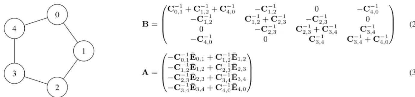
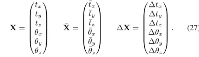
Figure 1 shows a simple graph containing five vertices and five directed edges. Each edge denotes a scan matching, where the model set corresponds to the 3D point cloud with an outgoing edge and the data set corresponds to the point cloud with the in-coming edge. For all points in the data set the closest point in the model set is calculated. Based on these point pairs the covariance matrices are estimated as stated above. The matrixBfeatures 4 entries, since the first 3D scan, i.e., scan 0, defines the coordinate system and is not transformed. However, the covariance matrices with index 0 appear in the loop closing and atB1,1
Following the convention in (Borrmann et al., 2008a), we
repre-sent a poseX, as well as its estimate and error, in Euler angles
X= tx ty tz θx θy θz ¯ X= ¯ tx ¯ ty ¯ tz ¯ θx ¯ θy ¯ θz
∆X=
∆tx ∆ty ∆tz ∆θx ∆θy ∆θz
. (27)
The matrix decomposition MiH = ∇Zi( ¯X)is given in Fig-ure 2. As required,Micontains all point information, whileH expresses the pose information. Thus, this matrix decomposition constitutes a pose linearization similar to that proposed in the pre-ceding section. While the matrix decomposition is arbitrary with respect to the column and row ordering ofH, this particular de-scription was chosen due to its similarity to the3D pose solution given in Lu and Milios (1997). Finally, a system of6(n−1) equa-tions (ndenotes the number of poses to be estimated) has to be solved, but since the pose graph is sparse the resulting equation system is sparse, too. We use a sparse Cholesky decomposition as SLAM back end (Borrmann et al., 2008b)
3. INCLUDING INFORMATION OF GROUND CONTROL POINTS
Arguably, the most important part of exploiting any available global truth data in static or kinematic 6D SLAM implemen-tations is the ability to fix a pose in the global relaxation step. As described previously, the globally consistent scan registration method with Euler angles fixes the zeroth scan while other scans are movable for registration (cf. Figure 1). This is usually the desired behaviour.
The first approach to pose fixing that was explored is the so called algorithmic approach. The main idea of this approach is to find a way to introduce the pose fixing functionality in the 6D SLAM algorithm without changing the way how the LUM with Euler angles works. In other words, without changing any mathematics behind the global relaxation algorithm.
The fixed scan version of 6D SLAM algorithm works similar to the global relaxation described above. Two additional steps are introduced. First, the graph is transformed to take into account the fixed scans. Namely, the nodes representing the fixed poses are merged with the zeroth node and the required link rearrange-ment is done.
After the graph is rearranged, the vector containing all scans has to be rearranged as well. Namely, a meta scan containing all fixed scans has to be created and set as the zeroth scan. After that all other scans have to be renumbered in a sequential manner accordingly. This has to be done to ensure proper generation of the matrices in the linear equation systemBX=A.
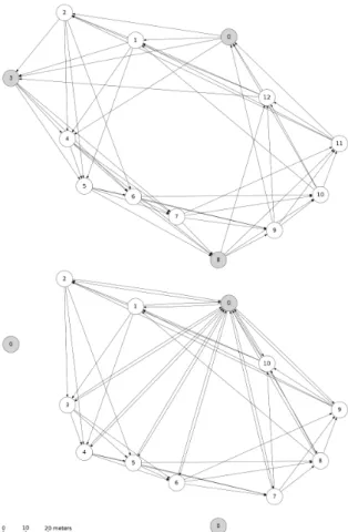
Figure 3 (above) depicts a typical graph for the SLAM problem. Each node is connected to a few further nodes as it is expected that there is a large enough overlap that lets these point clouds to be matched. The loop is closed, hence the last node is connected to the first node. The grey nodes need to be regarded as fixed. If this graph was passed to an unchanged LUM global relaxation algorithm, the grey nodes would be treated as any other. The way the LUM algorithm is defined, only the zeroth node is treated as fixed. Thus, to treat scans 3 and 8 in Figure 3 as fixed, the following actions have to be carried out:
Figure 3. Above: A typical directed graph for a SLAM problem. Each node is connected to a few further nodes that can be matched to it and the loop is closed. The grey nodes have to be regarded as fixed. Below: Structure of the graph after the scan fixing proce-dure has been applied. The fixed scans are now treated as a single metascan.
2. Add the edges pointing to and from the fixed nodes to the zeroth node.
3. Remove duplicate links.
Figure 3 (below) depicts the example graph discussed previously after the described procedure.
As opposed to the algorithmic approach to pose fixing, the mathe-matical approach strives to fix the pose by exploiting the way how the global relaxation is being done. In other words, although the graph object has to be changed slightly in order to convey the nec-essary information about which poses have to be fixed, the graph structure should not be changed. Instead, the global relaxation al-gorithm should make use of available information regarding fixed scans and construct the linear equation system accordingly.
Given the math in section 2.. It is important to note thatX rep-resents the concatenation of posesX1, . . . ,Xn. In other words, only the non-fixed poses compose the linear equation system BX = Aand are solved for. Thej andk in (21) represent columns and rows in the corresponding arrays and hence only in-clude movable nodes, the sums in 21 inin-clude the zeroth node as well through the use of indexl. While this is appropriate notation when only the zeroth node is fixed, if a graph with an arbitrary number of fixed nodes is considered, the notation has to be ex-tended. In this case, it is useful to use indexlto denote the set of
fixed nodes. Then equations (21) become:
Bj,k=
Pn
k=0C
−1 j,k+
Pn l=0C
−1
j,l (j=k) C−1
j,k (j6=k)
(28)
Aj= n
X
k=0,k6=j
C−j,k1E¯j,k+ n
X
l=0
C−j,l1E¯j,l (29)
whereC−1
j,l represent the covariance between thej-th movable and l-th fixed scans andE¯j,lis the corresponding observation. Then, the linear equation system (21) consists ofnequations and can be solved fornvariables, wherenis the amount of movable nodes. The graph edge information, as well as the neighbour relations between all nodes, including the fixed ones, is taken into consideration while building the matrixBandAaccording to (28). To build the linear equation system, a fully connected graph is considered where the covariance between two nodes that are not connected with an edge is set to zero.
4. EXPERIMENTS AND RESULTS WITH FIXED POSES
To test the functionality of the pose fixing methods, two exper-iments were carried out. In both cases data were gathered by a robot traversing the environment and stopping to make 3D point clouds. However, both cases have distinct environmental proper-ties allowing to highlight the differences between used methods.
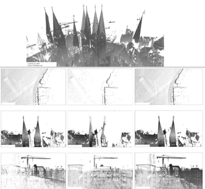
The first dataset used to verify the developed methods is a dataset recorded in Downtown Bremen, Germany. It contains a total of thirteen three dimensional point clouds generated using a RIEGL VZ-400 3D laser scanner. Each point cloud in turn contains up to 22.5 million points. The initial pose estimations needed for point cloud matching are provided by exploiting the odometry data of the robot. Figure 5. shows the result. One can see that the system cannot complete converge as the scans 0,3, and 8 cannot be moved.
Apparently, the difference that sets these two scan fixing algo-rithms apart in this situation has to be the final positions of the movable scans. This is easily explainable by using the graphs that have been used for both methods. The first difference is that the zeroth node in the graph used for algorithmic scan fixing contains all point clouds that have to be fixed as opposed to mathematical approach where the point clouds are treated as fixed yet separate. The second difference is the amount of links which is heavily re-duced in algorithmic scan fixing as opposed to mathematical scan fixing.
5. FROM FIXING SCAN POSES TOWARDS INCORPORATING GROUND CONTROL POINTS
In previous parts methods for doing simultaneous localization and mapping, as well as methods for denoting certain posed as fixed while doing SLAM have been described.
Let us consider a situation where a dataset has been acquired in a statical terrestrial manner using a 3D scanner and there are ground truth points along the path that can readily be identified in the dataset. In this situation each scan provides a 3D represen-tation of the surrounding environment in which zero to n ground truth points can be identified. The problem of aligning a pose with the underlying ground truth eventually boils down to find-ing a transformation between the set of the known ground truth points and the set of the corresponding points of the dataset. The criterion for reliable pose determination is to have at least three non-singular, non-linear ground truth points that can be identified in a single scan if current methods of determining a transforma-tion between two matchable point clouds are used.
Kinematic SLAM adds it’s own corrections both to pose fixing and the incorporation of ground truth data. While the underly-ing algorithm for the pre-processunderly-ing step is the same as for static SLAM, eventually the whole dataset is split up in smallest pos-sible slices where each slice has it’s own modifiable pose as de-scribed in Elseberg et al. (2013). More often than not it will be the case that it is not possible to identify three ground truth positions in a single slice to perform unambiguous data association.
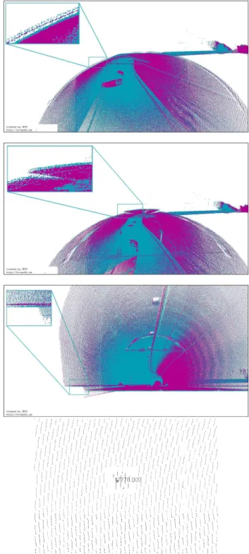
Experiments have been carried out on a tunnel dataset that con-tains 3D point cloud data taken using a LIDAR system consisting of two 2D laser scanners arranged in the typical ”X” formation and positioned on top of a car. Apart from point and trajectory information, the dataset comes with ground truth information. Ground truth points have been acquired using independent sur-veying methods. The ground truth coordinates point to a bolt head in the centre of a painted circle on the tunnel’s wall. Due to paint having different reflectance than the surrounding wall, the painted circle is an identifiable feature in the dataset. Due to separate point clouds being acquired by separate scanners and in separate runs, it is possible to compare datasets that should yield the same result and identify any discrepancies. Such comparison has been done and can be examined in Figure 4.
In future work, we aim at constraining the semi-rigid SLAM cor-rection, with ground control points. In typical setups there are merely three control points per segment visible, thus fixing scans at ground truth poses is not sufficient. A possible solution would be to include the ground control points as a fixed ”‘scan”’ and to incorporate a high weight of a matching between the extracted marker and these points.
6. CONCLUSIONS
This paper has presented methods for fixing scan poses in our globally consistent scan matching, i.e., our 6D SLAM optimiza-tion framework. Experiments confirm the applicability in several scenarions. Furthermore, we describe the real-world scenario of using ground control points in a tunnel mapping task.
References
Besl, P. and McKay, N., 1992. A method for Registration of 3-D Shapes. IEEE Trans. Pattern Analysis and Machine Intelligence (PAMI) 14(2), pp. 239–256.
Figure 4. Above: The two images from the top depict discrepan-cies found between point clouds acquired using different scanners on the same run. The third image shows discrepancies between point clouds acquired using the same setup on different runs. Dif-ferent colors denote difDif-ferent point clouds. Below: A ground truth point plotted together with data. The point’s coordinates point to a bolt head in the middle of the painted circle.
Borrmann, D., Elseberg, J., Lingemann, K., N ¨uchter, A. and Hertzberg, J., 2008a. Globally Consistent 3D Mapping with Scan Matching. Journal Robotics and Autonomous Systems (JRAS) 56(2), pp. 130–142.
Figure 5. Above: Non-registered input 3D point clouds. Below: Left column contains images created using the original global relaxation without pose fixing, middle column contains images taken from the same position with algorithmic pose fixing, right column contains images with mathematical pose fixing.
Campbell, J. B., 2002. Introduction to remote sensing. CRC Press.
Dubayah, R. O. and Drake, J. B., 2000. Lidar remote sensing for forestry. Journal of Forestry 98(6), pp. 44–46.
Elseberg, J., Borrmann, D. and N ¨uchter, A., 2013. Algorithmic solutions for computing precise maximum likelihood 3d point clouds from mobile laser scanning platforms. Remote Sensing 5(11), pp. 5871–5906.
Fernald, F. G., 1984. Analysis of atmospheric lidar observations: some comments. Applied optics 23(5), pp. 652–653.
Horn, B. K., 1987. Closed-form solution of absolute orientation using unit quaternions. JOSA A 4(4), pp. 629–642.
Lu, F. and Milios, E., 1997. Globally Consistent Range Scan Alignment for Environment Mapping. Autonomous Robots 4(4), pp. 333 – 349.
N ¨uchter, A. and Lingemann, K., 2011. 3DTK – The 3D Toolkit.
N ¨uchter, A., Elseberg, J., Schneider, P. and Paulus, D., 2010. Study of Parameterizations for the Rigid Body Transformations of The Scan Reg-istration Problem. Journal Computer Vision and Image Understanding (CVIU) 114(8), pp. 963–980.