Model
Amanda M. Bouffier1, Jonathan Arnold2*, H. Bernd Schu¨ttler3
1Institute of Bioinformatics, University of Georgia, Athens, Georgia, United States of America,2Genetics Department, University of Georgia, Athens, Georgia, United States of America,3Physics and Astronomy Department, University of Georgia, Athens, Georgia, United States of America
Abstract
Doing large-scale genomics experiments can be expensive, and so experimenters want to get the most information out of each experiment. To this end the Maximally Informative Next Experiment (MINE) criterion for experimental design was developed. Here we explore this idea in a simplified context, the linear model. Four variations of the MINE method for the linear model were created: MINE-like, MINE, MINE with random orthonormal basis, and MINE with random rotation. Each method varies in how it maximizes the MINE criterion. Theorem 1 establishes sufficient conditions for the maximization of the MINE criterion under the linear model. Theorem 2 establishes when the MINE criterion is equivalent to the classic design criterion of D-optimality. By simulation under the linear model, we establish that the MINE with random orthonormal basis and MINE with random rotation are faster to discover the true linear relation with p regression coefficients and n observations whenpwwn. We also establish in simulations withnv100,p~1000,s~0:01and 1000 replicates that these two variations of MINE also display a lower false positive rate than the MINE-like method and additionally, for a majority of the experiments, for the MINE method.
Citation:Bouffier AM, Arnold J, Schu¨ttler HB (2014) A MINE Alternative to D-Optimal Designs for the Linear Model. PLoS ONE 9(10): e110234. doi:10.1371/journal. pone.0110234
Editor:Fabio Rapallo, University of East Piedmont, Italy
ReceivedApril 14, 2014;AcceptedSeptember 16, 2014;PublishedOctober 30, 2014
Copyright:ß2014 Bouffier et al. This is an open-access article distributed under the terms of the Creative Commons Attribution License, which permits unrestricted use, distribution, and reproduction in any medium, provided the original author and source are credited.
Data Availability:The authors confirm that all data underlying the findings are fully available without restriction. All files are available from http://sourceforge. net by searching on the keyword: linearminesimulations.
Funding:Funded was provided by the National Science Foundation DBI-1426834. The funder had no role in study design, data collection and analysis, decision to publish, or preparation of the manuscript.
Competing Interests:The authors have declared that no competing interests exist. * Email: [email protected]
Introduction
The Problem: The researcher wishes to carry out model-guided
discovery about a system from a sequence ofnexperiments. The
challenge is that each of the n experiments performed is very
expensive, and so at each stage(nz1)it is desirable to design the
next experiment to be maximally informative. The approach in
whichnexperiments are to be done sequentially in such a way as
to capture the most information at each stage n about the underlying model is called utilizing the Maximally Informative Next Experiment (MINE) [1]. The method has been shown to be consistent for one version of MINE [2]. To understand MINE we
will consider the linear model, Y~Xbz", where Y is a n|1
vector of dependent measurements, X is a n|p matrix of p
independent variables, each with n measurements, b is a p|1
parameter vector, and" is a n|1 vector of independently and
identically distributed normalN(0,s2)errors.
The problem has four features. First, there are many parameters
and limited data(nvvp)so there will be many more unknown
parameters than data. In this setting a large sample of variables(p)
is to be observed as it is not known in advance which ones are
relevant. In fact, typicallyn*100whilep*103{106. Second, the
X matrix is partitioned into two parts,X~(X0,X00), whereX0is
ann|p0matrix of independent variables that the experimentalist
can control andX00 is ann|p00 matrix of independent variables
that cannot be controlled under the conditionsp~p0zp00[3]. The
X0matrix will be referred to as the design matrix. For simplicity,
we will assume the entireX matrix is made up ofX0. Third, the
next experiment encompasses stagesnz1,. . .,nzd, where d is
the dimension of the experiment. Experiments constitute batches
ofdobservations. The fourth and final feature of the experiment is
that each experiment ofd observations is very costly, be it time,
materials and/or subjects, or financially such as 250,000 per
experiment [4]. So at each stagenin the overall study, there is a
high premium on choosing the best next experiment. The problem
is to discover with reasonably high probability the modelbin as
few steps(n)as possible. We call this a problem in model discovery
because what we wish to know is what linear relation can be
discovered from the many variables (p) measured over the time
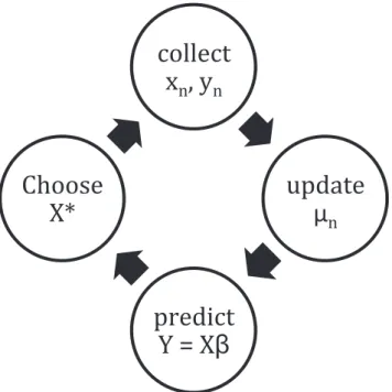
course of the study. Again the number of variables measured is large because it is not known in advance which ones are relevant. The process of discovering the model is cyclical as shown in Figure 1.
This problem makes points of contact with several distinguished problems in statistics and engineering. There are problems in experimental design [5,6,7,8,9] leading to model refinement with
n.p, particularly for sequential designs [10]. There are problems
As an example problem for use in model-guided discovery, suppose the researcher wishes to understand human longevity [12]. The researcher may examine the characteristics of US centenarians. Several thousand variables are measured including genetics, diet, and lifestyle on each centenarian because it is unknown which variable or variables have an effect on longevity. Some of these variables can be controlled, such as diet and lifestyle. Others, like the genes carried by the centenarian, cannot be controlled. In model refinement, the goal is to select a design,
X0(diet and lifestyle), to reduce the error in the parametersbby
consideration of, for example,X0TX [7] and its determinant (i.e.
D-optimality). In process control with the aid of response surfaces,
the goal might be to select a designX0to maximize the expected
longevityE(yi)(whereE()denotes expectation andyidenotes the
longevity of the ith individual in the study) by manipulating diet
and lifestyle. Such an engineering approach to extending lifespan has been implemented in the nematode [13]. In model-guided
discovery the goal is simply to choose a designX0at each stage to
discover the factors that determine longevity with as few
centenarians (n) as possible and using limited data, to discover
potentially many important variables.
Another example of this framework in systems biology can be seen in the description of genetic networks at a steady state or system in equilibrium [14]. In this setup a genetic network is approximated to first order by the following linear system:
dx
dt~Ax{y ð1Þ
Here the column vector x describes the concentration of
mRNAs of genes in a network, and theyvector describes external
perturbations. The A matrix captures the network relationships
among the genes, anddx
dt is the derivative with respect to time.
A steady state is assumed so that the dynamical system reduces to:
y~Ax ð2Þ
The problem is to infer the networkA. An experiment entails
measuring all mRNAs under a particular perturbation y, so several perturbations are tested. This setup reduces to a linear regression problem. Such design problems have been considered for nonlinear genetic network models as well [4,8,15,16], but we will not focus on these here.
Mathematical Results
Model Estimation by the Ensemble Method2
A standard approach to estimating the regression coefficientsb
is the least squares method. This approach reduces to solving the normal equations below for the least squares estimates of the
parameters^bb:
XTX^bb~XTY ð3Þ
The challenge in our problem is thatXTXwill not often be of
full rank because of collinearity in the independent variables and because there are so few data points relative to the number of
parameters(nvvp). While the normal equations in (3) could be
solved by use of a generalized inverse, there are likely to be many solutions that are equally consistent with the data and not one best
least squares estimate^bbof the parameters in the model. The key is
to not find one estimate, but rather an ensemble of estimates
consistent with the dataY.
To address this problem the likelihood is consulted at each stage:
L(bjY)~(2ps2){ n 2 e
{P
n
i~1 ½yi{P
p
j~1 Xijbj
2
2s2 ð4Þ
Since there are so many independent variables with so little data, this surface resembles a golf course with its varied terrain of many hills and sandpits than a mountain or mountain range. However, we can reconstruct the entire likelihood function by Markov Chain Monte Carlo methods (MCMC). By integrating
over a standardized L(b) with respect toband using a particular
prior distribution, we can make predictions about the behavior of the system even in the presence of such limited data [17]. So
instead of finding one best parameterbto represent the system,
instead we constructL(bjY) or alternatively, the entire posterior
distribution with a different prior distribution. These are special cases of the ensemble method, in which some figure of merit is used to select a distribution of models fitting experimental data [17], and as a special case the reconstruction of the standardized
L(bjY) is referred to as the ensemble. In this paper the
standardized likelihood can be calculated exactly when the
variance (s2) is known, the case to be used here, and with a
Gaussian conjugate prior onbfrom Eqn (4) (see ref [18]):
Figure 1. Cycle of MINE discovery – Simplified Computing Life Paradigm.
p(bjY)!(s2){ p 2e
½{(b{mn)T(X T XzL0)(b{mn)
2s2 ð5Þ
The posterior meanmnis described as:
mn~(XTXzL0)
{1(XTX^bbzL
0m0) ð6Þ
The least squares estimate^bbenters into the calculation of the
posterior meanmn. In the program description section below, we
replaceXTXbin (6) withXTY from (3).
Here the precision matrix which determines the prior
distribu-tion in (5) is L0 and will be taken asbI wherebis a positive
constant andIis thep|pidentity matrix. We also refer to this (5)
as an example of the ensemblep(bjY). In the past we have used a
uniform prior over a finite interval [17], but the Gaussian prior distribution insures that the integration can be done along all
components of the parameter vector(b)over the whole parameter
space and can approach that of a noninformative prior distribution by letting diagonal elements of this matrix become small.
Normally the moments of the ensemble would be calculated by MCMC methods [17], but from (5) we can obtain the moments of
b directly and for example the linear model with known error
variance.
Eb(b)~mn ð6Þ
Var(b)~s2(XTXzL0)
{1~C~B{1 ð7Þ
These moments of the ensemble can be updated as each observation is added.
Maximally Informative Next Experiment
At each stagen, we choose the next experimentXby reference
to the ensemble p(bjY) in (5) to infer the unknown but true
regression parametersb0. The new design matrix consists of d
rows, and after completion of the next experiment is used to
augmentXntoXnzd orXX~. The design of the new experiment is
captured in X and the augmented/updated design for all
experiments in XX~. For each member of the ensemble (b) we
make a prediction vector about thed outcomesYY^ of the next
experiment, namely YY^~Xb, where b is drawn from the
ensemble of models in (5),YY^is the vector ofdpredictions for the
next experiment, andXis the design of the next experiment. We
choose the new experiment X such that we have maximum
discrimination between the alternatives in the ensemble. If two random models of the ensemble should have correlated predicted
responsesYY^ for experimentX, the choice of design would be
poor as this would not reveal as much information as when two random members should have uncorrelated responses.
One MINE criterion for choice ofXwas developed by use of a
microscope analogy [4]. The object in the microscope isb0. The
image under the microscopeYY^is mapped onto the objectb
0in the field of the microscope, but the mapping is fuzzy and imperfect
with their being uncertainty inYY^. Let v
0 be a volume in the
object space (i.e., the parameter space Rp) under the light
microscope wherepis the number of parameters, and letvD be
the ‘‘image difference volume’’ swept out that is viewed. For a microscope, the connection between the two volumes is the model of physical optics. In our context here, the connection is the model
predictionYY^~Xb. Formally, the image difference volumevDis
swept out by the image difference vector DYY^(b,b0,X) for all
pairs of objects(b,b0)in(v0,v0)or
vD(v0,v00,X)~DYY^(v0,v00,X)~X(b{b 0
) ð8Þ
The image difference volume is swept out by varyingbandb0in
(8).
The image difference volume depends explicitly onv0and how
we ‘‘twiddle the dials’’ on the microscope though X. The
maximally informative next experiment (MINE) criterion is based
on this idea that the more volume invD(v0,X), the more detail
discerned inv0. This is achieved by adjusting the data captured in
X.
In order to take advantage of this MINE criterion, we must
make a selection of the object volumev0. The choice is improvised
but driven by computational practicality [4]; other choices are
possible [19]. We elect to define a ‘‘representative volume’’vD
swept out byDYY^(b,b0,X)whenbandb0
are drawn randomly as ‘‘typical’’ or average values from the ensemble pair distribution
p(b,b0jY)~p(bjY)|p(b0jY), the components given by (5). The
volume is constructed from the variance – covariance ellipsoid of
the image difference volumeDYY^(b,b0,X)and is dependent on the
choice of experimentX. We define the ensemble distribution of
DYY^(b,b0,X)as:
QD(W,X):~
ð
b
ð
b0
d(W{DF(b,b0,X))p(bjY)|p(b0jY) ð9Þ
The quantityWis any point in theDYY^(b,b0,X) volume and
d(:::)is the Dirac Delta Function. The ensemble distribution in (9)
specifies an effective difference volume vD(v0,X) in the image
difference spaceDYY^(b,b0,X)by way of the characteristic ellipsoid
of this space specified by:
Dik(X)~COV(YY^i,YY^
k)~
ð
W
1
2½WiWkpDYY^(W,X
) ð10Þ
The variance – covariance ellipsoid is centered at the origin,
W~0 because pDYY^(W,X
) is an even function in W due to
DYY^(b,{b0,X)~{DYY^(b,b0,X). The variance – covariance
ellipsoid has the D-matrix eigenvalues and directions of the half-axes given by the D-matrix eigenvectors. From (10) we can write the covariance ellipsoid in terms of the moments of the ensemble:
COV(YY^i,YY^k)~E(YY^iYY^k){E(YY^i)E(YY^k) ð11Þ
Normally these moments could be computed by MCMC methods [17], but because of the explicit form in (5) we can evaluate (11) directly from (5) as:
Table
1.
Parameters
for
simulations.
np
d
b0 b1 b2 b3 b4 b5 b6 b7 b8 b9 biw
9
s
,
1001
1000
10
11
–36
–26
9
33
–50
–45
15
3
17
0
0.01
doi:10.1371/journal.pone.
Figure 3. Graph of the number of significant nonzero regression coefficients averaged over 1000 replicates for: (A) the MINE-like method; (B) MINE method; (C) MINE method with random orthonormal basis; (D) MINE method with random rotation.Each graph identifies the number of replicates (y-axis) with a varying number of the nonzerob0components as significant as a function of the number of experiments (x-axis). Blue corresponds to 70% correctly identified, red to 80%, green to 90% and purple to 100%.
doi:10.1371/journal.pone.0110234.g003
Figure 4. Posterior means of the first 20 regression coefficients as a function of the number of experiments for: (A) the MINE-like method; (B) MINE method; (C) MINE method with random orthonormal basis; (D) MINE method with random rotation.Each panel is averaged over all 1000 simulations with 10 zero (in blue) and 10 nonzero (in red). The first ten (red) are truly nonzero.
X(XTXzL0){1s2XT~XB{1XT~XCXT ð12Þ
The matrixCis defined to beB{1. A Hilbert Space (HS,i.e., a
complete inner product space) formalism is introduced to give a compact form to the MINE criterion. The HS of functions consist
of functions defined on the model parameter space, fb:b"Rpg,
for which the covariance is the HS inner product. This inner product is formally defined as:
(gjh)~E½g(:)h(:){E½g(:)E½h(:) ð13Þ
The components of the observation vector,YY^
i, are represented
by:
fi(b):~f(b,YY^i) fori~1,:::,d ð14Þ
We can write the covariances in terms of the inner product:
Dik~(fijfk) ð15Þ
The ensemble standard deviation of the prediction YY^
i is
equivalent to the HS vector norm or length denoted byjjYY^
ijj. The
norm is defined byjjgjj:~(gjg)12
If the predictionsYY^
1,. . .,YY^d are linearly dependent, then the HS prism is defined by the predictions collapses to a lower
dimensional one, and the determinant det (D) vanishes. If the
predictions are not linearly dependent, then predictions determine an HS prism whose volume is simply given by the product of their
vector lengths, namelydet (D)~(jjYY^
1jj:::jjYY^njj) 2
. In general the predictions are correlated, and we have the Hadamard Inequality:
det (D)ƒ(jjYY^1jj:::jjYY^njj)2 ð16Þ
The ratio det (D)
(jjYY^
1jj:::jjYY^njj)
2 can be thought of as a composite
measure of the dependence of the predictions and is a function only of the HS angles between predictions.
We are now in a position to introduce a MINE criterion first by introducing the normalized predictions.
^ Z Zi~
^ Y Yi jjYY^ ijj
, i~1,:::,n ð17Þ
The normalized covariance matrix or correlation matrix denoted by R is defined by:
Rik(X)~(ZZ^ij^ZZ
k)~
Dik(X)
(jjYY^ ijj jjYY^kjj)
ð18Þ
~E½ZZ^(:,YY^i)ZZ^(:,YY^k){E½^ZZ(:,YY^i)E½^ZZ(:,YY^k)
This is the correlation matrix among the predictions. We
propose the following MINE design criterionV(X):
V(X):~det(R(X))~ det(D(X ))
(DDYY^
1DD:::DDYY^nDD)2
ð19Þ
This criterion is the squared volume of a prism spanned by the
normalized predictionsZZ^
1,. . .,ZZ^n. Such a criterion is advanta-geous when the predictions are almost but not actually/completely
Figure 5. The number of false positives as a function of the number of experiments.These numbers are averaged over all 1000 simulations for each method. Blue corresponds to MINE-like, red to MINE, green to MINE with random orthonormal basis, and purple to MINE with random rotation. The final two overlap almost exactly which is why the green line is not visible.
linearly dependent. This is a situation that has been encountered in practice [4]. This MINE criterion from (12) only depends on the ensemble through its variance-covariance matrix and not its mean in (6). The MINE criterion is also scale-free [4,20]. It clearly differs
from the usual model refinement criterion based on
XTXor XTX.
In practice the MINE criterion will behave better thanXTX
forn*100andp*1000because its calculation through inverting
Bis stabilized byL0in (12), as in Ridge Regression [21] and will
potentially incorporate the data from prior experiments in (12)
through theBmatrix. Its form also lends itself to optimization for
large problems as will be shown under Theorem 1 below and
under simulation results later(nvvp).
Maximizing the MINE Criterion
Ideally we would have a necessary and sufficient condition for maximizing the MINE criterion. Here in Theorem 1 we only present a sufficient condition for maximizing the MINE because the necessary condition has not been found.
Theorem 1:If the rowsXiof the design matrixXare chosen
to bewiC{1=2, wherewi,. . .,wdis any orthonormal set, then the
MINE criteriondet (XCXT)is maximized.
Proof:V(X)is maximized whenV(X)~1. This occurs if and
only if det (R)~1 which is only satisfied if and only if
(YY^
ijYY^k)~dikjjYY^ijj 2
from (19), where dikis the Kroneker delta.
From (13) the inner product can be used to represent the
covariances asDik~(YY^ijYY^kT). The conditiondet (R)~1is thus
equivalent to Dik~dikjjYY^ijj
2
or equivalently XiCXkT~
dikjjYY^ ijj
2
(TheX
i denotes the i
th
column ofX). We now need
to introduce two more equivalencies: wi~XiC1=2 and
wT
k~C1=2XkT. The fact that any positive semi-definite symmetric
matrix, such asC, has a square root gives us the liberty to create
such a wi. Since X
iCXkT~dikjjYY^ijj 2
, this leads to wiwTk~
dikjjYY^ ijj
2
, which implies any orthonormal basis can be used for w1,. . .,wd.
In particular, the vectors X1,. . .,Xn can be selected as the
eigenvectors ofConce standardized byC{1=2. One efficient route
for maximizing the MINE criterion is then simply to compute the
eigenvectors and eigenvalues ofCor equivalently, to maximize the
parallelpiped whose volume isdet (R) [4] and then to normalize
them byCinwi~XiC
{1=2~X
iB1=2. The choice of
normaliza-tion still needs to be examined as a model-guided discovery tool. See simulation results for examination of three choices of different orthonormal bases, a (1) normalized eigenvector basis; (2) random basis; (3) normalized eigenvector basis with random rotation.
Model Refinement
A traditional approach to choosing the designX(in contrast to
MINE) is to chooseXto maximize some simple function of the
variance-covariance matrix of the parameter estimates(b)such as
the determinant, to create a D-optimal design [6,8]. Consider then
the augmented design matrixXX~ which is not only a function of the
current design X but includes the possible design of the new
experimentX. This means:
~ X
X~(XT,XT)T~(X,X) ð20Þ
Under ordinary model refinement, we wish to minimize some
simple function of the variance-covariance matrix ofb, such as:
det (XX~TXX~zL0){1or equivalently
maximize det (XX~TXX~zL 0)
ð21Þ
This can be written explicitly in terms of the new experiment with the identity:
~ X
XTXX~~XTXzXTX ð22Þ
The model refinement criterion is then to maximize det (A)
where:
A~XTXzL0zXTX ð23Þ
The derivative ofdet (A)with respect to each component ofX
can be computed from:
+det (A)~tr(Adj(A))+A ð24Þ
Here the+is the gradient with respect toX,tr()refers to the
trace and Adj() denotes the Adjoint. A necessary condition for
maximizing thedet (A)is for+det (A)~0. This max determinant
(max det) problem is closely related to solutions to an affine formulation of this max det problem, and the problem is most
closely related to the analytic centering problem [22]. These
authors cast the search for D-optimality in design as a convex
optimization problem with the max det problem linear inXand
with linear inequality constraints [22]. The linearity in X is
achieved by constructingX from a set of rows (or designs) that
are known in advance. The optimization problem is then reduced to determining how often each row (design) is used. Here we do not know the rows in advance.
MINE can produce a D-optimal Design
Kiefer and Wolfowitz [23] established that D-optimal designs are equivalent to mini-max designs, which minimize the maximum of the expected loss associated with each possible design. It is natural to ask whether or not there is any such relation between D-optimal designs and MINE. While the model refinement procedure appears to start from an entirely different criterion than MINE, it is possible to establish a relation between these different kinds of optimal designs by imposing the same constraints on the respective optimization problems. When we do this, we can establish:
Theorem 2 (Equivalence Theorem of D-optimality and
MINE):The MINE procedure in Theorem 1 is D-optimal in the
sense that X maximizes det (A) subject to the constraint
XjCXiT~1whereA~XTXzL0zXTX.
Proof: In order for MINE and a D-optimal solution to be directly comparable they need to be maximized subject to the
same constraints on X. So we maximize det (A) subject to the
following constraint from (12):
Max det (A) subject toXjCXT
i ~1 ð25Þ
The constraint insures the columns ofX are an orthonormal
basis.
We can introduce a related criterionGG~(X)as:
det (BzXTX)
~det (B1=2) det (B1=2) det (B{1=2(BzXTX)B{1=2)
~det (B) det (IzB{1=2XTXB{1=2)
~det (IzWTW)~GG~(X) whereW~XB{1=2
Note that det (A)~GG~(X)=det (B). So maximizing det (A) is
the same as maximizingGG~(X). The maximization problem in (25)
is equivalent to:
MaxGG~(X)~det (IzWTW) subject to wjwi~1 for j~1,. . .,d
ð26Þ
The constant d is the number of observations in the new
experiment. We can think of the original optimization problem as
equivalent to determining the best set of normalized vectorswj.
From (26), the constraints imply thattr(WTW)~dwheredis
the dimension of the next experiment (i.e., the number of
observations in the next experiment). We also have the trace
being the sum of the eigenvalues ofWTW.
tr(WTW)~X d
v~1
lVtr(WTW)~
Xd
v~1
lv~d ð27Þ
Constraint (27) implies a constraint on the eigenvalues in (27), but not the converse. To finish the proof we will first maximize
G(X)subject only to (27) reminiscent of [22].
We will then show the solution of this max det problem can also be chosen to satisfy all of the constraints in (26).
WTW~X d
j~1
wTjwj where dvp ð28Þ
Sincedvp, we can choose at leastp{dorthonormal vectorsuv
such that:
WTWuv~0 v~p{dz1,. . .,p ð29Þ
We choose theseuvvectors also to be orthogonal tow1,. . .,wd.
We will call this subspace of the parameter space as the
unexplored subspace. Note that while rank(WTW)ƒd, but
dimension (WTW)~p (that is, pwd here). This implies that
p{deigenvalues are zero. (This implies that forp{deigenvalues,
say forv~p{dz1,. . .,p, are zero. As an example, ifp~1000
andd~10, then the last 990 of the eigenvalues are zero. We have
lv~0 forv~p{dz1,. . .,p ð30Þ
These degenerate eigenvalues in (30) are associated with the unexplored subspace. This fact along with the determinant being the product of the eigenvalues implies from (26):
G(X)~
P
dv~1(1
zlv) ð31Þ
Now maximizeG(X)with respect tol
1,. . .,ld only subject to constraint [27] using the method of Lagrange multipliers (with
multiplierW). We find that:
l1~l2~ ~ld~ G(X)
W {1 and
Xd
v~1
lv~d ð32Þ
These two imply thatlv~1 for v~1,. . .,d on the explored
subspace of the parameter subspace.
The result of maximizing with respect to the eigenvalues is that
WTW is diagonalized with only the first d diagonal elements
being 1. The maximum value ofG(X)is 2dfrom (31).
From here, if we choosew1,. . .,wd to be an orthonormal set
such that wjwTk~djk, then we have WTWwj~wj for all
j~1,. . .,d. Thuswj is an eigenvector ofWTW with eigenvalue li~1for j~1,. . .,d. All constraints in (26) are satisfied for the solution to the max det problem with (27).
Choice of prior distribution
The choice for the prior mean vector is reasonably taken as zero since most of the independent variables are not expected to have an effect on the dependent variable y. The only question is
the choice of b specifying the precision matrix inB~ XT XzL
0
ð Þ
whereL0~bI(and specifies the prior). Dumouchel and Jones [24]
provide one argument to select b with an idea to making the design robust to violations of linear model assumptions. We will suggest another approach.
Let XTX have eigenvaluesliwith corresponding orthonormal
eigenvectors ui. Then we can write XTX and B as:
XTX~XliuiuTi ð33Þ
B~XðlizbÞuiuTi ð34Þ
XTXui~li ð35Þ
uTiuj~dij ð36Þ
The eigenvalues ofBarelizband have the same eigenvectors
asXTX. We can now introduce a new variable:
pi:~uTib ð37Þ
We can loosely think of the uncertainty or standard deviation of
theb-vectors (across the ensemble) in theuidirection as:
si:~s(pi)~b
{1=2
i ~(lizb)
{1=2 ð38Þ
In the absence of any experimental data(li~0), the uncertainty
in theuidirection should reduce to:
si(prior)~b{1=2 ð39Þ
We would expect the uncertainty without experimental constraints (of data) to exceed the uncertainties with data or that:
si(prior)wwmin (si) equivalently bvvmax (li) ð40Þ
The maximum eigenvalue ofXTXprovides an upper bound on
b. This one would be satisfied, for example, ifbwere chosen to be
equivalent to the weight of one observation inX0X. The matrix
X0X would quickly dominate. The next constraint is more
stringent, and so it is not necessary to check that (40) is satisfied.
Another constraint on barises from the requirement that the
true regression coefficients not be too far out in the tails of the
prior distribution; otherwise the data throughXTXwill never find
the true regression coefficients. We can think of the prior distribution as equivalent to a fishing-net. We want this net to be well cast to catch the fish.
Introduce bmax~max (jtruebkj)~max (jE(bk)j) where the
expectation is taken over the ensemble. Then the b-value should be chosen so that
si(prior)wwbmax ð41Þ
This is equivalent to requiring:
bvv 1
b2max ð42Þ
So with the prior data,XTX, and some idea of the magnitude
of the regression coefficients, there are constraints on the prior
distribution as specified by the precision matrix and hence b.
These constraints are satisfied in the simulations to follow. As an example, if the largest magnitude of a regression coefficient were
50, thenbvv 1
502orbvv0:0004. Since we set all variables and
know the largest regression coefficient’s magnitude is 50, we set
b~0:0001. This is a tighter constraint than the first. We also do
not wantbto be too small to allowCin (12) to still be inverted as
Methods
Methods for simulating four versions of MINE under the linear model
The program MINE to simulate the above procedures is written in Java under version 1.6 and utilizes the version 5 of the Jama library [25]. Details of the input and output of this software are already reported [26]. The program is available in sourceforge.net under the name linearminesimulations. There are four variants on the MINE method described below in this section and summa-rized in Figure 2.
Following the initialization of many variables (including but not
limited to the matrices and vectors to store theXmatrix,Ymatrix
ande, the number of variables(p)and the significance matrix) and
the set up of data from the input file, the main part of the simulation program begins. Since the first experiment has no data on which to base a design, this pilot experiment is randomly generated. The simulation program is designed to handle a variety of data. If the number of variables is over 50, then the first experiment is selected to have 10 observations; otherwise, the first experiment has between five and nine observations. The number of pilot observations varies between 0 and 10 as determined by the number of variables. Each value in the pilot is created by generating a random number between 0 and 10 and then dividing
it by thepvalue. The set is not then normalized nor orthogonal.
After the pilot experiment is generated, the random number generator is changed depending on which method is used in order to allow for the same pilots but the rest of the numbers generated
being different. From here the first set of the dependentYvector is
calculated along with the associated error vector ("). With the
initial data generated the real calculations can begin.
Each loop (in which a single observation is added) first consists of calculating the posterior mean (6) and then calculating the
significance of the regression parameters inbwith the cycle exiting
here if the number of loops reaches the target number of
experiments. The mean ormnis calculated by (6). Although in this
simulation we have the true valuesb0, we useXTY in (6) rather
than using the real value or the previous mean. The significance
subroutine takes the most recently calculated mean mn and the
whole X matrix. It solves for the posterior variance-covariance
matrix ofbwith (7) with the wholeXmatrix and multiplies this by
s2. Thez-value of eachbis calculated with each individual mean
value divided by the square root of the diagonal of the above
matrix. The p-value is then calculated using thisz-value. Thesep
-values are then sorted from largest to smallest. The resulting -values are checked using a Benjamini-Hochberg method [27] to decide
which components ofbare significant. The calculation forp-value
is done using the algorithm from Press et al. [28] (on p. 221). From here, depending on the specific method in Figure 2, the new
observations are calculated, and finally the new Y vector is
calculated byY~Xbz"and the cycle repeats in Figure 1. The
error vector (") or error values are created by generating a
standard normal random variable value and multiplying it bys
(which was set by the input file).
MINE-like method. The simple naı¨veMINE-like methodtakes the
ten eigenvectors of the C matrix in (7) associated with the ten
largestC-eigenvalues using a common subroutine to generate the
Cmatrix and simply uses these eigenvectors to generate the next
X.
MINE Method. TheMINE methodsimply uses the eigenvectors
associated with the C matrix as above with the ten largest
eigenvalues and multiplies the corresponding eigenvectors by the
square root of theBmatrix to obtain the nextX.
MINE with Random Orthonormal Basis. In MINE with a random orthonormal basis a set of ten random orthonormal vectors is
generated and then standardized by the square root of the B
matrix(B1=2). First, the ten vectors are created from using the
random orthonormal set subroutine. Then each individual vector
is multiplied by the square root of theBmatrix to obtain the next
X.
MINE with Random Rotation. The MINE with a random rotation
method first finds all the eigenvectors in theCmatrix as above but
selects the set of all degenerate vectors instead of simply the ten largest. Then the method creates a random orthonormal array of
Q|Q where Q is the number of degenerate eigenvectors to
multiply the degenerate matrix with. This is used to rotate the degenerate eigenvector set. The first ten are then multiplied by the
square root ofBmatrix and used to obtain the nextX.
The randomly generated orthonormal set used in both the MINE with a random orthonormal basis and MINE with random rotation is done by first generating a single vector of random Gaussian values. The vector is then normalized to a unit vector. This vector is used as the basis for generating more vectors generated in the same method and is made orthogonal using a modified Gram-Schmidt (MGS) algorithm [29].
To obtain the square root of the B matrix, first C in (7) is
calculated. Then the square root of C is solved by using the
Singular Value Decomposition(VTDV)where theVmatrix here
is the eigenvectors in column form and theDmatrix is a diagonal
matrix with the square root of the eigenvalues on the diagonals. This is then inverted by the method in the Jama package [25] to
get the square root ofBmatrix.
With each of the four methods the same set of 1000 components
of the trueb0were used. Thisb0only had ten components that
were truly nonzero. The order of the nonzero components was not changed in the list of 1000 components. These were the first ten
values ofb0and were as follows: 11,236,226, 9, 33,250,245,
15, 3, and 17. The program was run with1000 replicates for each
of the four methods. Each replicate had a unique pilot experiment (consisting of ten observations), but these pilot experiments were the same for each method, allowing for a stronger comparison of the four methods. Each individual run had a unique random seed
so that the rest of the replicate run would be unique. The errors
in the linear model used was 0.01, and all of the prior mean values
(m0)were initialized to zero. A summary of the parameters in the
simulations is given in Table 1.
Results of Simulation
There are four variations on the MINE procedure examined here and defined in the previous section. The similarities and differences in the pathways of the four methods are summarized in Figure 2. All four methods employ the same subroutines for the majority of their implementation but differ in the way each particular method chooses the next experiment or set of observations to use, as described in the program description above. The first method is called the naı¨ve MINE or MINE-like
method because this version does not incorporate theB matrix
used in Theorem 1. This simpler method only calculates the
eigenvectors ofC and uses the eigenvectors with the ten largest
eigenvalues (according to the algorithm) to define the next
experiment X. The second method, MINE, takes the
MINE-like method and simply multiplies the chosen eigenvectors byB1=2.
The third method, called MINE with random orthonormal basis, does not use calculated eigenvectors as suggested by
Theorem 1 from, for example, matrix C. Instead, the third
method creates a set of random orthonormal vectors and
standardizes this basis byB1=2. This method allows us to examine
the effect of choice of the orthonomal basis in Theorem 1 on the performance of MINE. The final method tested is called MINE with random rotation. This method combines the previous methods by taking the chosen set derived in the MINE method but rotates the set by a random orthonormal basis before standardizing using a modified Gram-Schmidt Algorithm [29]. In contrast to the MINE method selecting an orthonormal basis, which is a function of the machine precision in the calculation of
the eigenvectors and eigenvalues of C, the MINE with random
rotation removes this dependence on the machine precision as the ‘‘randomizer’’ and replaces the resulting choice of eigenvectors (axes) with a random spin of the axes defined by the eigenvectors
of theCmatrix.
There were a number of criteria considered for comparing the MINE methods. These criteria include (1) identifying the nonzero
values of b0 by using a Benjamini-Hochberg multiple test
correction [27] at a 1% significance level, (2) identifying the
correct sign and value for the nonzero components ofb0, and (3)
determining the number of false positives.
The first criterion discerns if the methods correctly identify the
nonzero values ofb0as being significant or successful discovery as
given by the test described above. A method is considered better or more successful the fewer experiments are needed to discover the truly nonzero regression coefficients. In Figure 3 there are four graphs provided (A–D) to display this criterion, and all iterations performed are shown.
The MINE-like method seems to perform the poorest in this criterion (Figure 3A) in that successful discovery was very late. However, being satisfied with a lower percentage of correctly included independent variables (say 7 out of 10) allows for more replicates meeting this criterion. The method began mostly (over
50% of the replicates) identifying 7 of 10 at the 87th experiment
and only at the 90th experiment did over 90% of the replicates
identify 7 of 10 of the true components ofb0. For over 90% of the
replicates to identify all nonzero values of b0 at least 97
experiments were required.
The other three methods performed significantly better than the MINE-like method. The MINE method performed almost twice as fast in this criterion as the MINE-like method (Figure 3B). For
example, over 50% identified 7 of 10 at the 45thexperiment and
over 90% at experiment 50. Only 63 experiments were required for over 90% of the replicates to identify 9 of 10 experiments.
However, to get all nonzero values of b0 required much more
time. Sixty-six experiments were needed to get over 50% and 83 experiments before over 90% of the replicates considered significant.
Both the MINE with random orthonormal basis and the MINE with rotation performed almost identically (Figures 3C and 3D).
Both identify 90% of the nonzero values of b0 in over 900
replicates at the 47thexperiment. However, attempting to identify
all ten nonzero components of b0 in all samples requires much
more data, similar to the MINE method. It takes more than 80 experiments for both of these methods to identify all nonzero
values ofb0in over 800 of the replicates.
The second criterion involved identifying the correct sign and value for the nonzero beta values. This is evaluated by methods described earlier. Figures 4A–4D depict an average value for the first 20 values where the first ten are the nonzero coefficients and
the second ten are zero and are shown as a comparison. As previously discussed, early detection is important.
As in the previous criteria the MINE-like method performed
poorly (Figure 4A). After the pilot experiment the nonzero b0
values have the correct sign identified and never change sign
though the full run of experiments; however, the experimentalb0
values do not reflect the components of the true vectorb0until the
final experiment. Also interestingly the values increase slowly until
about experiment 85 when the absolute value of each b
component drastically increases towards the true value.
MINE performs similarly in pattern to the MINE-like method. MINE does just as well at sign detection, with no real variable ever offering the incorrect sign (Figure 4B). The pattern of the MINE is less gradual than the MINE-like but features a slow growth then a sudden spike and approaches the asymptote of the true value. The MINE reaches the slope change between experiments 50–55 and so it takes the remaining 45–50 experiments to arrive at the plateau of the real value.
The other two methods also outperform the MINE-like method. Again, in this criterion the MINE with random orthonormal basis and the MINE with random rotation perform almost identically (Figures 4C and 4D). Sign identification seems to be the easiest criterion as these two also perform flawlessly here. Unlike the previous two, these methods seem to have a very linear pattern in
the values of theb0nonzero components.
The next criterion involves comparing the false positives of each
method (Figure 5). A false positive happens if any of theb0that
are actually zero are considered significant. For comparison, the average number of incorrectly identified values, averaged over all simulations for each method, is shown.
Again, we see similar patterns where the MINE-like method performs poorest. Initially, it looks like it is performing adequately, since up until experiment 60 there are zero false positives. Since we have to wait until experiment 85 for any reasonable amount of success, we find that the false positives are beyond 400 and at some of the highest peaks compared to the other three methods. The only way this method could possibly be considered better is that it drops off faster at the final observed experiment but since this point is a worst case, this point should not be reached.
The MINE method has a similar pattern to the MINE-like, again performing in a similar scaled manor. At the point where information could be accepted for the nonzero values, around experiment 55, the false positive rate is around 300 which would allow for about 70% of the variables to be eliminated. If more experiments are performed, the number identified peaks just under 460 during experiments 73–84 afterwards it gradually begins dropping.
The MINE with random orthonormal basis and MINE with random rotation again display almost identical results. However, in contrast to the MINE-like and MINE methods, these two have a more linear growth of false positives, especially after the first 15 and before the last 15 experiments. Due to the data being displayed on a single graph, the similarities are more observable with the two lines eclipsing each other. During the most optimal selection periods between experiments 20–45, the false positives do not go over 225. This allows for a greater than 75% reduction in variables. These two do however peak ever so slightly higher with the average reaching just under 465 but a much later experiment and are only lower during a 20–30 experiment window. All simulation results in Figures 3–5 are summarized in an excel file generated with the program MINE under the keyword linear-minesimulations at sourceforge.net.
outperform the other two procedures, we conclude by examining the properties of the MINE with random rotation, namely its power and false positive rate, in a situation with increased noise in Table 2. Not unexpectedly with more noise it takes a larger number of experiments before the power to detect 7 out of 10 true regression coefficients are significant is large as the noise
(measured bys) is increased. The false positive rate is controlled
when one stays below the number of experiments necessary to obtain 7 out of 10 true regression coefficients most of the time. As
an example, for asof 0.05 and a power of 98.3% in Table 2, the
false positive rate is only 0.94%.
Discussion
In 2008 a key problem in systems biology was solved as identified by Kitano [30] with a new methodology called MINE [4]. The MINE methodology is used to integrate several cycles of modeling and experiments to yield discoveries about the under-lying process being studied. The result of the application of the MINE methodology was new insights into the relation of the clock to ribosome biogenesis [1,4]. This new approach to model-guided discovery has sparked a flurry of developments in MINE methodology [19,31,32,33]. It is natural to ask how this new experimental design methodology of MINE is related to classical experimental design criteria and whether or not we can validate MINE mathematically as a discovery tool when there are many
parameters and sparse, noisy data (pwwn). A natural place to
validate this new MINE tool is in the framework of the oldest and mostly widely used statistical model, the linear model.
One of the consequences of the work here is to establish another view of one MINE procedure. When the same constraints are imposed on MINE and the D-optimality criterion, then the MINE procedure discussed here is D-optimal under the linear model. The effect of minimizing the determinant of the correlation matrix of the predictions is equivalent to minimizing the determinant of the variance-covariance matrix of the parameter estimates as described in detail in the Equivalence Theorem 2 when the same constraints are imposed on both problems. We suspected this would be the case from the application of the MINE procedure in systems biology, where the application of the MINE procedure
appeared to decrease the estimated error variances2 over time
[4]. In the language of the microscopy analogy, maximizing the volume observed under the microscope by choice of experiment is equivalent to reducing the ellipsoid of variation in the optical field of the parameter space. It is this key relation that Marvel and Williams exploit to address Kitano’s problem [19].
Having shown the MINE procedure in practice is useful for discovery [4], it is natural to ask how MINE performs in a simpler setting of the linear model. We explored its performance under
four variations. In this simpler setting, where we can actually calculate the ensemble directly without resorting to using Markov Chain Monte Carlo as used in nonlinear systems [34], we can solve the associated optimization problem of MINE in Theorem 1 in a way that may suggest new approaches to MINE in nonlinear models. The result of Theorem 1 was the realization that the maximization of the MINE criterion here is defined up to an orthonormal basis of the data space. There are a variety of different bases that could be selected. Theorem 1 also calls for a standardization of the basis. This standardization does prove important as we see upwards of a 50% improvement in some criteria between the MINE-like and the MINE methods.
First, it was important to see the two more similar methods (MINE with random orthonormal basis and MINE with random rotation) performed similarly. Second, these two proved better in all of the criteria in almost all experiments. These allowed for the earliest detection, during which they provided the closest to true values on all variables, and provided the fewest false positives for a larger sample reduction. The only area at which these two methods were out performed was in the number of experiments needed for most of the simulations to identify the real values given that initial detection had begun. The MINE method once 10% of the simulations began detecting these values was able to reach 90% more quickly. Though this region was smaller for the MINE method, the other two were not only able to reach or arrive at the 10% quicker but generally complete (get over 90%) quicker.
A third consequence of this work is to open up a new convex programming problem that is closely tied to the max det problem so thoroughly analyzed by Boyd and co-workers [22]. The argument here in the max det problem is quadratic in the design parameters with linear inequality constraints potentially as opposed to an affine argument. An open question is whether or not this new problem is a convex programming problem. If so, then much of the machinery developed by Boyd and coworkers could be developed for the problem here. We have illustrated the use of the convex programming procedure in our discussions in this work.
In conclusion, we feel that the MINE discovery tool has opened up many exciting design problems that will transform the way scientists now integrate theory and experiment in a number of areas beyond systems biology [3,35,36].
Author Contributions
Conceived and designed the experiments: AB JA HBS. Performed the experiments: AB HBS. Analyzed the data: AB JA HBS. Contributed reagents/materials/analysis tools: AB HBS. Contributed to the writing of the manuscript: AB JA HBS.
References
1. Chakrabarty A, Buzzard GT, Rundell AE (2013) Model’based design of experiments for cellular processes. Wiley Interdisciplinary Reviews: Systems Biology and Medicine 5: 181–203.
2. Dinh V, Rundell AE, Buzzard GT (2014) Experimental Design for Dynamics Identification of Cellular Processes. Bulletin of the Mathematical Biology 76: 597–626.
3. Lopez-Fidalgo J, Garcet-Rodiguez SA (2004) Optimal experimental designs when some independent variables are not subject to control. Journal of the American Statistical Association 99: 1190–1199.
4. Dong W, Tang X, Yu Y, Nilsen R, Kim R, et al. (2008) Systems biology of the clock in Neurospora crassa. PLoS One 3: e3105.
5. Fisher RA (1935) The design of experiments. Oliver and Boyd, London. 6. Kiefer J (1959) Optimum experimental designs. Journal of the Royal Statistical
Society Series B (Methodological): 272–319.
7. John PWM (1971) Statistical Design and Analysis of Experiments. MacMillan, NY.
8. Federov VV (1972) Theory of Optimal Experiments. Academic Press, NY.
9. Box EP, Hunter JS, Hunter WG (2005) Statistics for Experimenters. Wiley, NY. 10. Tsay J-Y (1976) On the sequential construction of D-optimal designs. Journal of
the American Statistical Association 71: 671–674.
11. Box EP, Draper NR (1998) Evolutionary Operation. Wiley, NY.
12. Poon LW, Jazwinski M, Green RC, Woodard JL, Martin P, et al. (2007) Methodological considerations in studying centenarians: lessons learned from the Georgia centenarian studies. Annual review of gerontology & geriatrics 27: 231.
13. Sagi D, Kim SK (2012) An engineering approach to extending lifespan in C. elegans. PLoS Genet 8: e1002780.
14. Gardner TS, di Bernardo D, Lorenz D, Collins JJ (2003) Inferring genetic networks and identifying compound mode of action via expression profiling. Science 301: 102–105.
16. Dette H, Melas VB, Pepelyshev A, Strigul N (2003) Efficient design of experiments in the Monod model. Journal of the Royal Statistical Society: Series B (Statistical Methodology) 65: 725–742.
17. Battogtokh D, Asch DK, Case ME, Arnold J, Schuttler HB (2002) An ensemble method for identifying regulatory circuits with special reference to the qa gene cluster of Neurospora crassa. Proc Natl Acad Sci U S A 99: 16904–16909. 18. Box EP, Tiao GC (1992) Bayesian Inference in Statistical Analysis. Wiley, NY. 19. Marvel SW, Williams CM (2012) Set membership experimental design for
biological systems. Bmc Systems Biology 6: 21.
20. Dette H (1997) Designing experiments with respect to ’standardized’ optimality criteria. Journal of the Royal Statistical Society: Series B (Statistical Methodol-ogy) 59: 97–110.
21. Draper NR, Smith H (1966) Applied Regression Analysis. Wiley, NY. 22. Vandenberghe L, Boyd S, Wu S-P (1998) Determinant maximization with linear
matrix inequality constraints. SIAM journal on matrix analysis and applications 19: 499–533.
23. Kiefer J, Wolfowitz J (1960) The equivalence of two extremum problems. Canadian Journal of Mathematics 12: 234.
24. DuMouchel W, Jones B (1994) A simple Bayesian modification of D-optimal designs to reduce dependence on an assumed model. Technometrics 36: 37–47. 25. Mathworks T (1998) JAMA: A Java Matrix Package[Java reference library] version 1.0.2 August 1998. Available: http://mathnistgov/javanumerics/jama/. 26. Bouffier A (2013) A MINE Alternative to D-Optimal Designs for the Linear
Model. M Phil Dissertation, University of Georgia.
27. Benjamini Y, Hochberg Y (1995) Controlling the false discovery rate: a practical and powerful approach to multiple testing. Journal of the Royal Statistical Society Series B (Methodological): 289–300.
28. Press WH, Teukolsky SA, Vertterling WT, Flannery BP (1992) Numerical Recipes in C, 2nd Edition. Cambridge University Press, NY, NY.
29. Bjork A, Paige CC (1992) Loss and recapture of orthogonality in the modified Gram-Schmidt algorithm. SIAM journal on matrix analysis and applications 13: 176–190.
30. Kitano H (2002) Systems biology: a brief overview. Science 295: 1662–1664. 31. Donahue M, Buzzard G, Rundell A (2010) Experiment design through
dynamical characterisation of non-linear systems biology models utilising sparse grids. IET Syst Biol 4: 249–262.
32. Liepe J, Filippi S, Komorowski MC¸ , Stumpf MP (2013) Maximizing the
information content of experiments in systems biology. PLoS Comput Biol 9: e1002888.
33. Dinh V, Rundell AE, Buzzard GT (2014) Experimental Design for Dynamics Identification of Cellular Processes. Bulletin of Mathematical Biology 76: 597– 626.
34. Yu Y, Dong W, Altimus C, Tang X, Griffith J, et al. (2007) A genetic network for the clock of Neurospora crassa. Proc Natl Acad Sci U S A 104: 2809–2814. 35. Townsend JP, Leuenberger C (2011) Taxon sampling and the optimal rates of
evolution for phylogenetic inference. Syst Biol 60: 358–365.