Delaunay refinement for curved complexes

(1)

Universidade Federal de Minas Gerais Department of Electrical Engineering

Delaunay refinement for curved complexes

Adriano Chaves Lisboa

Advisor: Prof. Rodney Rezende Saldanha

Co-advisor: Prof. Ricardo Hiroshi Caldeira Takahashi

(2)

(3)

Abstract

(4)

(5)

Resumo

(6)

(7)

About this thesis

This work takes my name as author, but many people were important for its ac-complishment. I would like to thank:

• my family for the unconditional support throughout the course;

• my advisor, Professor Rodney Rezende Saldanha, for his enthusiastic and en-couraging help in my research, and for the dreamful advices I will carry for my life;

• my co-advisor, Professor Ricardo Hiroshi Caldeira Takahashi, for his kind attention and meaningful review of this text;

• Professor Renato Cardoso Mesquita for the friendly talks, which have changed the theme of this thesis;

• Professor Luis Gustavo Nonato for his valuable remarks during the qualifying exam;

• Professor Hani Camille Yehia for the free clues;

• Douglas Alexandre Gomes Vieira, Xisto Lucas Travassos Júnior, Sérgio Lu-ciano Ávila, Alexandre Ramos Fonseca, and Guilherme Parreira for the part-nership and friendship;

• CAPES and CNPq for the research encouragement.

Everybody output according to their knowledge, and input according o their knowledge. An eternal loop of creation and recreation in global networks. Not surprisingly, I am not likely to be the first one to publish these ideas. I do not know how many ideas you will miss in this text by thinking they are not here when I wished to tell you, or how many you will create by thinking they are here when I did not noticed, or how many other combinations I missed in this phrase. That is part of the magic.

(8)

(9)

Resumo estendido

Introdu¸c˜

ao

Uma malha pode ser vista como uma parti¸cão de um dom´ınio em elementos geral-mente simples e de um mesmo tipo. Ela pode ser aplicada em diversos contextos, como visualiza¸cão gráfica e interpola¸cão. Como foco de aplica¸cão de malhas neste trabalho, está o método de elementos finitos para solu¸cões de equa¸cões diferenciais parciais. Este método é bem restritivo quanto aos requisitos de malha, de modo outras aplica¸cões devem ser capazes de usar o mesmo gerador de malhas.

Para que o método de elementos finitos funcione, a malha deve possuir as pro-priedades topológicas definidas no conceito de complexo. Para que o método de elementos finitos atinja uma solu¸cão suficientemente precisa com o menor número de elementos, existem diretivas gerais que um gerador de malhas deve satisfazer. Primeiramente, um bom gerador de malhas deve ser capaz de gerar elementos não achatados, pois elementos achatados tendem a ser maus interpolantes e a gerar er-ros numéricos (em alguns casos especiais é interessante ter elementos achatados em certas dire¸cões). Outro ponto é que um bom gerador de malha deve ser idealmente capaz de gerar a malha com o menor número de elementos poss´ıvel, e refinar pos-teriormente onde for necessário. Esse refinamento deve suportar boas grada¸cões, de modo que a densidade de elementos em uma região não interfira significativamente em outra com densidade diferente.

Quando se tem apenas um gerador de malhas que lida com geometrias planas, é necessário fazer uma aproxima¸cão linear da entrada antes de gerar a malha. Em um contexto adaptativo, a informa¸cão de como deve ser a aproxima¸cão linear da entrada não é conhecida a priori. Neste caso torna-se imprescind´ıvel que o gerador de malhas seja capaz de lidar com geometrias curvas, onde as aproxima¸cões das partes curvas são devidamente refinadas onde for necessário no decorrer do processo.

Dentre as estratégias para gera¸cão de malhas, o refinamento Delaunay ocupa lugar de destaque pela sua elegância e garantias teóricas. Este trabalho estende o refinamento Delaunay para complexos curvos de entrada em dimensões arbitrárias. Para tanto, são estabelecidos dois teoremas principais. Um relacionado com o con-ceito de fortemente Delaunay e que estabelece condi¸cões para que um simplexo perten¸ca ao complexo simplicial Delaunay. Os algoritmos de Ruppert e de Chew são descritos sob o ponto de vista deste teorema. O segundo teorema é uma extensão da idéia fundamental do algoritmo de Bowyer-Watson para inser¸cão incremental em um complexo simplicial Delaunay. Existem também contribui¸cões na parte de

(14)

menta¸cão, como a busca em leque, a avalia¸cão de predicados robustos em dimensões arbitrárias e a determina¸cão de um ponto de Voronoi sobre pe¸cas curvas.

Defini¸c˜

ao de dom´ınios

Um PLC [Miller et al., 1996] (piecewise linear complex) define uma geometria for-mada por partes lineares, como sugere o nome. Neste trabalho, esta defini¸cão é estendida para partes curvas como um k-complexo de variedades definido por uma cole¸cão den-variedades, n= 0, ..., k, conectadas não vazias e disjuntas entre si, onde partes de mesma dimensão são desconexas entre si (o prefixo em complexo e em va-riedade representa a respectiva dimensão). As diferen¸cas fundamentais na defini¸cão de um k-complexo de variedades para a de um PLC é que as pe¸cas passam a ser variedades (potencialmente curvas), quek-pe¸cas também podem ser definidas e que as pe¸cas são conjuntos abertos ao invés de fechados.

Qualquer dom´ınio pode ser particionado em um complexo de variedades de maneira ´unica, como ilustrado nas Figuras1e 2.

n= 2 n= 1 n= 0 n= 0, 1, 2

Figure 1: Exemplo de um dom´ınio bidimensional (esquerda) particionado em um 2-complexo de variedades (direita).

n= 2 n= 1 n= 0

n= 3

Figure 2: Exemplo de um dom´ınio tridimensional (esquerda) particionado em um 3-complexo de variedades (direita).

Um complexo de variedades Ck _{´e aquele onde todas a variedades membro s˜ao}

Ck_{. A defini¸cão de complexo de variedades garante que ele seja} _C0_{. Para atingir} complexos de variedades Ck _{pode-se definir as partes onde a} _n_{-ésima derivada é}

descont´ınua como variedades independentes, n _≤k, como ilustrado nas Figuras3 e 4. Dessa maneira propriedades diferenciais s˜ao descritas explicitamente no complexo de variedades.

(15)

CONTENTS ₁₁

n= 2 n= 1 n= 0 n= 0, 1, 2

Figure 3: Exemplo de um dom´ınio bidimensional (esquerda) particionado em um 2-complexo de variedades C1 _(direita).

n= 2 n= 1 n= 0

n= 3

Figure 4: Exemplo de um dom´ınio tridimensional (esquerda) particionado em um 3-complexo de variedades C1 _(direita).

todas a pe¸cas tenham a configura¸cão topológica de uma bola, particionando partes que não sejam se necessário.

A A

B

B A B

C A

A A

A B

B

C

A A

A

B A B

B

A

Figure 5: Exemplo de diferentes tipos de configura¸cões topológicas de 2-variedades. Da esquerda para a direita: plano, tudo, esfera, toro and fita de Möbius.

Refinamento Delaunay

Um complexo simplicial pode ser definido como um complexo de variedades onde cada pe¸ca ´e um simplexo e onde as facetas de cada simplexo tamb´em fazem parte do complexo, como ilustrado na Figura 6.

(16)

n= 2 n= 1 n= 0

Figure 6: Exemplo de um 2-complexo simplicial.

o diagrama de Voronoi definido por Georgy Voronoi em 1908 [Voronoi, 1908]. O diagrama de Voronoi é um complexo de células compostas por todos os pontos que estão mais perto de um ponto do que qualquer outro ponto de um dado conjunto.

Considerando que cadak-pe¸ca do diagrama de Voronoi emRn_{est´a equidistante a}

exatamenten₋k+1 pontos (caso degenerado se forem mais den₋k+1 pontos), ent˜ao cada k-pe¸ca do diagrama de Voronoi est´a unicamente relacionada com um (n₋k )-simplexo do respectivo complexo simplicial para o mesmo conjunto de pontos, como ilustrado na Figura 7.

Figure 7: Diagrama de Voronoi e complexo simplicial de Delaunay para o mesmo conjunto de pontos.

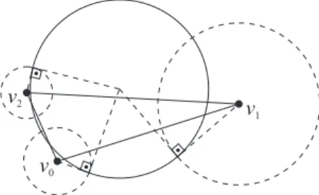
Em 1981 David Watson [Watson, 1981] provou que se uma k-pe¸ca, k > 0, do diagrama de Voronoi é degenerada, então existe pelo menos uma (< k)-pe¸ca degene-rada. Dessa maneira, um Diagrama de Voronoi é degenerado se e somente se existir pelo menos um vértice equidistante a mais de n+ 1 pontos. Um complexo simpli-cial de Delaunay dual a um diagrama de Voronoi não degenerado é dito fortemente Delaunay. Este complexo simplicial pode ser visto como aquele onde cada simplexo membro possui uma bola circunscrita que não contém nenhum outro vértice sobre seu contorno ou em seu interior.

(17)

CONTENTS ₁₃

circunscrita vazia então ele faz parte do complexo simplicial fortemente Delaunay, caso contrário ele não pode fazer parte. Esta propriedade é provada por Shewchuk em sua tese [Shewchuk, 1997] apenas parak = 2 e utilizando uma outra estratégia. Este teorema será denominado daqui para frente de teorema do fortemente Delau-nay.

Em 1987 William Frey [Frey, 1987] introduziu a inser¸cão no circuncentro de um simplexo, originando o refinamento Delaunay (ver Figura 8). Este refinamento possui a propriedade de não criar arestas menores caso forem escolhidos apenas circuncentros de simplexos que possuem circunraio maior que sua menor aresta. Em espa¸co bidimensionais, isto implica que este refinamento pode gerar garantidamente triângulos com ângulos diedros no intervalo [30o_,₁₂₀o_{]. Infelizmente em dimensões} maiores que a segunda não é poss´ıvel definir limites em medidas de qualidade válidas.

Figure 8: Refinamento Delaunay em uma triangula¸c˜ao.

Utilizando a propriedade de não criar menores arestas, Paul Chew propôs em 1989 [Chew, 1989b] o primeiro algoritmo de refinamento Delaunay para complexos lineares bidimensionais com garantias teóricas de qualidade. Este algoritmo pré-segmenta a entrada de maneira que todos os vértices se encontram a uma distância [h, h√3] entre si, e depois refina todos os triângulos com circunraio maior queh, como ilustrado na Figura 9. Sob o ponto de vista do teorema do fortemente Delaunay, isto garante que os segmentos de entrada terão uma circunc´ırculo vazio através do processo, e portanto farão parte da triangula¸cão. Este algoritmo pode ser estendido para dimensões arbitrárias de maneira direta, mas o processo de pré-segmenta¸cão o torna inviável na maioria dos casos práticos.

Em 1994 Jim Ruppert [Ruppert, 1994] propôs um algoritmo que não necessitava de pré-segmenta¸cão da entrada, dando garantias teóricas de qualidade, grada¸cão e tamanho para as triangula¸cões. Sob o ponto de vista do teorema do fortemente Delaunay, este algoritmo primeiro garante que cada aresta representando a entrada terá um c´ırculo diametral vazio (assim ela fará parte da triangula¸cão), e depois refina a triangula¸cão até que critérios sejam atingidos, como ilustrado na Figura 10. A idéia fundamental é que as arestas representando a entrada são refinadas caso seus c´ırculos diametrais sejam invadidos. A primeira etapa é denominada recupera¸cão de facetas, e a segunda de refinamento. Este algoritmo pode ser estendido para dimensões arbitrárias de maneira direta e ainda continua prático.

(18)

Figure 9: Malhas inicial (esquerda) e final (direita) geradas com o primeiro algoritmo de Chew.

Figure 10: Malhas inicial (esquerda) e final (direita) geradas com o algoritmo de Ruppert.

malha inicial gerada é então refinada até atingir critérios de parada. O comporta-mento deste algoritmo está ilustrado na Figura 11. O refinamento considera o caso especial onde a inser¸cão de um nó em um segmento causa a intercepta¸cão com outro segmento. Neste caso o segmento interceptado é refinado ao invés do segmento que o interceptou.

Para lidar com complexos curvos em dimensões arbitrárias, este trabalho revisita o algoritmo de Ruppert. Essa nova abordagem permite que a malha seja criada dimensão por dimensão, e que o refinamento possa ser feito em qualquer dimensão simultaneamente.

(19)

CONTENTS ₁₅

Figure 11: Complexo curvo de entrada esquerda), malha inicial (acima-direita), malha refinada para qualidade (abaixo-esquerda) e malha refinada para melhor qualidade e precis˜ao de representa¸c˜ao (abaixo-direita).

mais baixas para dimensões mais altas. Antes de passar para a dimensão seguinte, os simplexos da dimensão corrente são refinados até que bolas circunscritas pré-estabelecidas sejam vazias, garantindo que eles farão parte dos complexos simpliciais de dimensão superior. Nesta constru¸cão, cada pe¸ca do complexo de variedades define apenas um espa¸co paramétrico cujas restri¸cões e fronteiras são dadas por pe¸cas de dimensão inferior. Esta etapa está exemplificada na Figura 12.

(20)

Figure 12: Alguns passos da recupera¸c˜ao de facetas para um complexo de variedades (esquerda).

na Figura 13. Assim, pelo teorema do fortemente Delaunay, elas farão parte do complexo simplicial Delaunay juntamente com os respectivos simplexos de maior dimensão formados. As bolas circunscritas vazias que garantem a presen¸ca dos novos simplexos podem não ser as pré-estabelecidas, de modo que os vértices que possivelmente invadirem estas bolas deverão ser removidos.

a b

c B

Figure 13: Se a bola diametral B _{do segmento} _ab _{´e vazia, ent˜ao o subsegmento} _ac

tamb´em ter´a uma bola circunscrita vazia tangente a B _em _a _{desde que} _c_∈B_.

Implementa¸c˜

ao

Cada pe¸ca do complexo de variedades é armazenada em um mesmo vetor e sua posi¸cão nele a identifica. Cada pe¸ca contém uma representa¸cão paramétrica com respectiva dimensão, as pe¸cas vizinhas como ilustrado na Figura 14(para a gera¸cão de malha é suficiente que sejam armazenados apenas os vizinhos de dimensão in-ferior), e uma semente que será usada para identifica¸cão de simplexos membros.

(21)

CONTENTS ₁₇

Figure 14: Estrutura de dados (direita) para o complexo de variedades (abaixo-esquerda) para um dom´ınio de entrada (acima-(abaixo-esquerda).

de dimensão imediatamente inferior, e que o ponteiro para a variedade conformada é de obrigatória presen¸ca.

Figure 15: Estrutura de dados (direita) para o complexo simplicial (abaixo-esquerda) homeom´orfico a um complexo de variedades (acima-esquerda).

´

E utilizada uma versão estendida do algoritmo de Bowyer-Watson para fazer a atualiza¸cão do complexo simplicial Delaunay. Neste processo, a inser¸cão de um novo vértice gera uma cavidade, formada pelos simplexos invadidos, cujo contorno, denominado horizonte, é conectado ao novo vértice para originar os novos simplexos. Para atualizar os vizinhos dos simplexos do horizonte foi desenvolvida neste trabalho uma busca em leque, a qual está graficamente ilustrada na Figura16. Nesta busca, a faceta do simplexo do horizonte oposta ao vértice cujo vizinho relacionado se deseja determinar, é o “vértice” do leque. A busca segue então pelos vértices da cavidade conectados ao “vértice” do leque.

O predicado que diz de qual lado está um ponto em rela¸cão a um hiperplano, assim como aquele que diz se um ponto está dentro ou fora da bola circunscrita de um simplex, é dado pelo sinal do determinante de uma matriz. Pode-se escrever que o sinal do determinante calculado com erros de arredondamento está correto sempre que

(22)

f f e₁ f e₂ f e₀

neig ( )_f i i

v_i= facet ( )_f i

facet ( )e₂ p₂ p₀

q₀

q₂

p₂ p₁ _q

1

Figure 16: Representa¸c˜ao gr´afica da busca em leque.

ondeAné a matriz do predicado na n-ésima dimensão, ǫé a precisão da máquina, e

αn´e o permanente dos valores absolutos de An. Os coeficientes an para o predicado

de orienta¸cão em rela¸cão ao hiperplano são dados por

n

2(n+ 1) +n−1 (2) e para o predicado de orienta¸cão em rela¸cão à bola são dados por

n

2(n+ 1) + 3n+ 2 (3) Para calcular o ponto sobre uman-pe¸ca equidistante aos v´ertices de umn-simplex foi derivado neste trabalho um processo iterativo de Newton-Raphson dado por

tk+1 =tk−

fk f′ k T f′ k

f_k′

=tk−

cT kck

2(c′

kck)Tc′kck

c′_kck

(4)

ondet∈[0,1]n_{é o vetor de parâmetros,}_k_{é a itera¸cão corrente,}_f₍_t_{) =}_k_c₍_t₎_k2

é uma fun¸cão distância, c(t) é a proje¸cão da n-pe¸ca no n-plano do n-simplex transladada para o circuncentro, e f′₍_t₎

∈Rn _e_c′₍_t₎ _∈Rn×n _{s˜ao os respectivos gradientes (}_c′₍_t₎

cont´em como colunas os gradientes das componentes de c(t)).

Na Figura 17estão malhas para um complexo curvo com 44 pe¸cas refinadas sob diversos critérios. A malha é refinada a cerca de 400 nós/segundo sobre a superf´ıcie, e a cerca de 5.000 nós/segundo sobre o espa¸co tridimensional. Uma parti¸cão do 3-complexo simplicial é mostrada na Figura 18.

(23)

CONTENTS ₁₉

Figure 17: Malhas para o complexo curvo (acima-esquerda): sem refinamento com 26 nós (acima-direita), refinada aleatoriamente mantendoℓ/R≥1/√2 com 801 nós (meio-esquerda), refinada pela maior aresta com 729 nós (meio-direita), e refinada para representa¸cão precisa da geometria de entrada mantendo ℓ/R ≥ 1/√2 com 2006 nós (abaixo).

Conclus˜

ao

(24)

Figure 18: Parti¸c˜ao de um 3-complexo simplicial homeom´orfico a um complexo curvo.

0 10 20 30 40 50 60 70 80 90 100 110 120 130 140 150 160 170 180

0 200 400 600

dihedral (º) triangles

0 10 20 30 40 50 60 70 80 90 100 110 120 130 140 150 160 170 180

0 500 1000 1500 2000

dihedral (º) tetrahedra

Figure 19: Histograma de ˆangulos diedros de triˆangulos e tetraedros de um 3-complexo simplicial refinado pela maior aresta.

(25)

CONTENTS ₂₁

0 10 20 30 40 50 60 70 80 90 100 110 120 130 140 150 160 170 180

0 500 1000 1500 2000

0 10 20 30 40 50 60 70 80 90 100 110 120 130 140 150 160 170 180

0 2000 4000 6000 8000

Figure 20: Histograma de ângulos diedros de triângulos e tetraedros de um 3-complexo simplicial refinado para representa¸cão precisa mantendo ℓ/R_≥1/√2.

0 10 20 30 40 50 60 70 80 90 100 110 120 130 140 150 160 170 180

0 500 1000 1500 2000

0 10 20 30 40 50 60 70 80 90 100 110 120 130 140 150 160 170 180

0 2000 4000 6000 8000 10000

(26)

(27)

Chapter 1 Introduction

Defining roughly in a single sentence, a mesh is a partition of a geometric object into small pieces of simple shapes. Concrete illustrative examples are a honey comb, a mosaic, a spider’s web, or a woven - that suggests the name (see Figure 1.1).

Figure 1.1: Illustrative examples of meshes: honey comb, mosaic, spider’s web and woven.

A mesh embues simplicity to the geometric object it represents. The locality of its elements enables approximating assumptions inside their domain. For example, each piece in a mosaic may be considered to own a single color. Furthermore, the definition of shapes and connectivity as simple entities is the key for the development of a simple general mathematical framework, that is fundamental in computational applications. For example, a woven arrangement may represent any shape of cloth and provide uniform local features to it.

Numerous applications may be cited for meshes. A graphical engine uses meshes to represent complex geometric objects, so that shading models, projective transfor-mations or ray tracing may be fast cast on them. Meshes may interpolate nonuni-form samples of a function or a shape using their nodal connectivity. This work emphasizes on the investigation of a mesh generator algorithm for use in numerical methods to solve partial differential equations, like the finite element method. The requirements are very strict in this class of application, so that many of its mesh concepts are useful in other classes.

In focus in this thesis as a mesh generator, is the Delaunay refinement algo-rithm, that has theoretical guarantees on size, grading and quality supporting its good performance in practice. This algorithm generates simplicial meshes and most theoretical guarantees consider piecewise linear complex inputs. The main theme and results are in the extension of this algorithm for piecewise curved complexes.

(28)

1.1 Good meshes and mesh generators

Elements are the basis of a mesh. A good mesh have elements with properties and placement inside the domain that satisfy the problem requirements. A good mesh generator must be able to generate good meshes in a sufficient flexible process.

Lying in the context of numerical methods to solve partial differential equations, a mesh of the problem domain is used to create an interpolating function over it. Typically, physical properties are assigned to disjoint regions of the domain, boundary conditions are set on some lower dimensional parts of the domain, and then the ruling partial differential equations are forced to be satisfied within each element with boundary conditions defined by neighbor elements. The nodal values of the interpolating function are then given by a global system of linear equations.

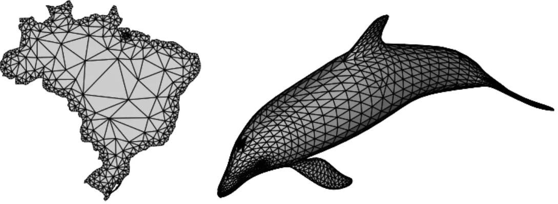
An output mesh must conform the input features of the domain it represents or approximates (see Figure1.2). Hence, each subset required in the problem domain must have a representative version in the mesh. If an input piece is linear, then an exact representation must be in the mesh. However, if an input piece is curved, then a homeomorphic approximate representation must be in the mesh, considering that the mesh elements are linear like simplices or boxes.

Figure 1.2: Triangular mesh of the Brazilian territory and surface triangular mesh of a dolphin.

Connectivity is also a key in numerical methods for partial differential equation solutions. It must hold general enough to represent any input domain connectivity, but it must be simple enough to allow a systematic and computationally efficient interactivity within the neighbors of each element. The most used connectivity con-straints for meshes are the basis of the well known definition of simplicial complexes. Output meshes can be required to be finer in some regions and coarser in others, so that the interpolating function accurately approximates the problem solution with fewer elements (see Figure 1.2, where an accurate boundary representation is achieved). Hence, refinement and grading must be supported by the mesh generator. A quasi-uniform mesh is in Figure1.3c and a grading mesh is in Figure1.3d, for the same input piecewise linear complex. This feature is known as grading optimality.

(29)

1.2. WHY CURVED COMPLEXES? ₂₅

mesh generator must be able to generate meshes not too finer than the coarsest possible mesh for an input domain. Where and when the mesh will be refined must be under user control. For instance, a mesh generator whose coarsest mesh is the one in Figure 1.3c is worse than the one that is able to generate the one in Figure 1.3b. This feature is known as size optimality.

(a) (b)

(c) (d)

Figure 1.3: Some examples of meshes for the same input geometry (left).

Due to numerical and interpolation errors, elements are required to look as round as possible. Two too close vertices, in relation to other vertices in the element, increase machine roundoff errors. A vertex too close to a facet, in relation to the facet size, is very likely to cause high interpolation errors and gradients in a linear interpolation. For instance, the mesh shown in Figure 1.3a is worse than the one in Figure 1.3b. This feature is known as mesh quality. Grading optimality and mesh quality are conflicting objectives. Nonetheless very good tradeoffs are possible in practice. There are specific problems where skinny elements aligned to the flow direction lead to much improved results. These anisotropic meshes deserve and have received attention, but they will not be discussed in this text.

Every aforementioned desirable property for meshes is unlikely to be better at-tained by a structured mesh than by an unstructured one. Even though, because of its simplicity, faster generation and point location, some applications still justify the usage of structured meshes. Simplicity and speed are always desirable in algorithms, as long as all requirements are satisfied.

1.2 Why curved complexes?

Inputting only piecewise linear complexes requires any curved object in the domain to be firstly approximated by flat objects. This breaks the mesh generation into two well defined steps. However, because it is a requirement of the mesh generator, the conversion is sometimes considered to be a modeling task. Treating curved objects like real curved objects during the mesh generation makes clear what is modeling and what is meshing. The geometric model will only have to answer questions made by the mesh generator.

(30)

elements than necessary. If the input is underrefined, any point insertion on it will consider the linear version of it, not the curved one. Furthermore, if the mesh generation is refined according to an adaptive strategy using the problem solution, any size guess will not be reasonable (otherwise the term adaptive is not applicable) and input remeshing will eventually be inevitable.

Another important point is that the input is a constraint. If skinny elements are in the input, they will have to be also in the output mesh. That could happen even if the curved objects did not feature any small angle between their facets. Unfortunately, only 2-dimensional meshes are not prone to this.

The best feature achieved by a mesh generator for curved complex inputs is coarser output meshes. Where and when the mesh will be refined is user defined. However, the input will never be exactly represented in the mesh, so that the curved model must always be queried, and even detecting the moment to query the curved model spends time.

1.3 State of the art

Since its beginning in 1987 with the circumcenter point insertion [Frey, 1987], many extensions have been proposed to conform the Delaunay mesh refinement to geomet-ric objects. The most remarkable ones are the Chew’s 1st algorithm [Chew, 1989b], Ruppert’s algorithm [Ruppert, 1994] and Chew’s 2nd algorithm [Chew, 1993]. All of them have been developed for the triangulation of planar straight line graphs, and the latter two were extended for the tetrahedralization of piecewise linear complexes in Shewchuk’s thesis [Shewchuk, 1997]. Recent studies have been pub-lished on triangulations [Boivin and Ollivier-Gooch, 2002] and tetrahedralizations [Borovikov et al., 2005, Cheng et al., 2007b] for curved geometric objects. Never-theless, mesh generation for this kind of input is still a wide open problem. A brief history up to the current stage is given next.

The nowadays known as Delaunay condition for simplicial complexes was pro-posed in 1934 by Boris Delaunay [Delaunay, 1934]. The first Delaunay triangulation algorithm was curiously published, unaware of their realization, by Frederick et al. [Frederick et al., 1970]. In 1977 Lawson [Lawson, 1977] proposed the flip Delaunay triangulation incremental algorithm and proved that it maximizes the minimum angle. In 1981 Bowyer and Watson [Bowyer, 1981, Watson, 1981] published an n -dimensional Delaunay incremental algorithm based on cavities. A generalized con-cept of Delaunay triangulation was introduced by Lee in 1978 [Lee, 1978], which was named constrained Delaunay triangulation by Paul Chew in 1989 [Chew, 1989a]. In 1998 Shewchuk [Shewchuk, 1998] proposed a definition for constrained Delau-nay simplicial complexes and stated a condition for their existence in higher di-mensions. Chew also introduced in 1993 a Delaunay criterion over curved surfaces

[Chew, 1993], which was generalized in 1994 by Edelsbrunner and Shah [Edelsbrunner and Shah, 1994]. Chen and Bishop [Chen and Bishop, 1997] proposed a Delaunay criteria for curved

(31)

1.3. STATE OF THE ART ₂₇

in the range [30o_,₁₂₀o_{], where the lower bound is only violated near small input} angles. In this algorithm, the input piecewise linear complex must be segmented to the edge length range [h, h√3] and the output mesh is quasi-uniform, as shown in Figure 1.4.

Figure 1.4: Initial (left) and final mesh with 2293 triangles (right) generated by Chew’s first algorithm.

(32)

theoret-ical guarantees (see Figure 1.7), but without quality nor size guarantees. The algo-rithm requires input dihedral angles greater than 60o _{between input edges, greater} than 69.3o _(arccos√₂_/₄_≈₆₉_.₃o_{) between input edges and planes, and greater than} 90o _{between input planes. Shewchuk also conjectured that, in higher dimensions,} Ruppert’s algorithm terminates for ℓ/R_≤2(1−d)/2 _{with good grading.}

Figure 1.5: Initial (left) and final mesh with 426 triangles (right) generated by Ruppert’s algorithm.

Figure 1.6: Input piecewise linear complex with small angles (left) and respective mesh (right) created with Ruppert’s algorithm.

(33)

1.3. STATE OF THE ART ₂₉

Figure 1.7: Input piecewise linear complex (left) and cut on the final tetrahedral mesh (right) generated by Ruppert’s algorithm.

has the same basis of Ruppert’s algorithm by replacing the diametral circles by lenses, and considering the constrained triangulation. This algorithm guarantees output angles in the range [26.57o_,₁₂₆_.₉o_{] (arcsin 1}_/√₅ _≈ ₂₆_.₅₇o_{), [28}_.₆o_,₁₂₂_.₈o_] with Miller et al. analysis [Miller et al., 2003], and requires the same input angle constraints as Ruppert’s algorithm. The second Chew’s algorithm for tetrahedral-izations [Shewchuk, 1997] terminates for shortest edge length to circumradius ratios no smaller than√6/4≈0.6124 with grading guarantees. Shewchuk also conjectured that, in higher dimensions, Chew’s second algorithm terminates for ℓ/R _≤ p3/2d

with good grading.

(34)

Figure 1.8: Input curved complex left), initial mesh with 14 triangles (top-right), mesh refined for quality with 80 triangles (bottom-left) and mesh refined for boundary accuracy with 284 triangles (bottom-right).

a manifold and the restricted Delaunay simplicial complex for samples over it. The algorithm was latter simplified [Cheng et al., 2007a] to one that guarantees an out-put homeomorphic restricted simplicial complex as samples on inout-put get denser.

A guaranteed quality Voronoi refinement algorithm for anisotropic triangular mesh generation was proposed by Labelle and Shewchuk [Labelle and Shewchuk, 2003], and extended for domains with curves by Yokosuka and Imai [Yokosuka and Imai, 2006].

(35)

notori-1.4. MAIN RESULTS AND OVERVIEW OF THE THESIS ₃₁

ously axis aligned. This algorithm was generalized in 2000 to higher dimensions by Mitchell and Vavasis [Mitchell and Vavasis, 2000].

Figure 1.9: Triangular mesh (right) generated from the quadtree decomposition (left).

Some approaches to mesh generation are physically based on particle simulation, usually with analogy to bubble packing [Yamakawa and Shimada, 2000] or spring network [Persson, 2005]. They start with a crude mesh and improve the quality forcing equilibrium or finding the minimum entropy point. The high quality output meshes, as the example shown in Figure 1.10 from the mesh generator for implicit geometries developed by Persson [Persson, 2005], are extremely well graded and sized. Such a great result comes at a price and is limited. The points must be well distributed from the beginning, otherwise a local minimum may trap the algorithm. The update is expensive because all vertices must be moved in every iteration, and the number of iterations is theoretically unbounded. It is not natural to conform boundaries separating sub-domains or any lower dimensional object other than the domain contour. They usually use the Delaunay criterion on their connectivity scheme. All these features essentially define this approach as a mesh optimization process for interior points, where there are no guarantees to reach good results for arbitrary input geometries, but start meshes will not get worse.

1.4 Main results and overview of the thesis

(36)

Figure 1.10: Initial (left) and final (right) mesh generated by physical simulation.

representation. Some differential and topological properties for a manifold complex are sketched, as well as its computational representation.

Shewchuk has proven in his thesis that a triangulation is strongly Delaunay if there exists a circumcircle, for every edge, that contains no other vertex of the triangulation other than the edge endpoints. In this work this theorem for strongly Delaunay simplicial complexes is extended to higher dimensions by stating that a simplicial complex is strongly Delaunay iff codimensional simplices are strongly Delaunay, for any single dimension.

With the theorem just stated at hands, the Chew’s and Ruppert’s algorithms are revisited and presented in the point of view of protecting balls. Under this perspec-tive a Delaunay refinement algorithm for curved complexes arises more naturally.

A generalization of the fundamental idea of the Bowyer-Watson algorithm is the basis of the generalization of the Ruppert’s and Chew’s second algorithm for dealing with manifold complexes. This extension is presented as a theorem and guarantees that simplices representing input pieces will be part of the simplicial complex throughout the meshing process. It is proposed a feasible algorithm with expected theoretical guarantees on termination and quality.

(37)

Chapter 2 Domain representation

In the finite element method, the partial differential equations are discretely solved over a bounded domainS_⊂Rn_{, as shown in Figure}_{2.1, which may be disconnected}

and contain lower dimensional parts. Disconnected parts may represent indepen-dent problems, or may be virtually connected through boundary conditions. Lower dimensional parts represent thin objects, where a suitable formulation is applied.

Figure 2.1: A bounded domain in R2 _{where the finite element method is applied}

(left) and some subsets inside it (right).

The setS _{must be represented by a collection of subsets (see Figure}_{2.1). These}

subsets are assigned to physical properties, or boundary conditions... or whatever the problem requires. This chapter defines an unambiguous partition of S_{, in order}

to guarantee a nice representation of its features.

2.1 Manifold complex

Before defining the fundamental idea of the domain partition - the manifold com-plex -, some basic definitions and concepts are first introduced to let the text self-contained and to ease comprehension.

Definition 1 (disjoint) Two sets are disjoint iff they have no element in common.

Definition 2 (cover) The cover of set aS_{is a collection of nonempty non-duplicated}

subsets whose union is S_.

Definition 3 (partition) A partition of a set S_{is any} _cover _of S _{in which subsets}

are pairwise disjoint.

(38)

Definition 4 (neighborhood) A neighborhood of a point p is any set containing a ball centered at p and with radiusǫ >0.

The neighborhoodof a point introduces into a set the very simple, but also very important, concept of open and closed.

Definition 5 (open set) A set is open iff any point in it has a neighborhood lying in the set.

Definition 6 (closed set) A set is closed iff any point outside it has aneighborhood disjoint from the set.

Definition 7 (closure) The closure of a set is the smallest closed set containing it.

Definition 8 (boundary) The boundary of a set S _{is the intersection between the}

closure of S _{and the closure of the complement of} S_.

The idea of open sets brings to small scales the concept of infinite, like in the definition of limits. The infinitely far is where anything beyond makes no difference but there is always something beyond. The infinitely close is where anything in between makes no difference but there is always something in between. When the boundaries of a set are taken away, what remains includes something infinitely close to it, which characterizes an open set.

Definition 9 (topological space) A topological space is a set X _{together with a}

collection of open subsets _T that satisfies the conditions

1. _{∅ ∈ T}

2. X_{∈ T}

3. The intersection of a finite number of sets in T is also in T.

4. The union of an arbitrary number of sets in _T is also in _T.

(39)

2.1. MANIFOLD COMPLEX ₃₅

k= 2 k= 1 k= 0

k= 3

Figure 2.2: Examples of k-manifolds projected on the plane.

Definition 10 (k-manifold) A k-manifold is a topological space where there is a

neighborhood around every point that is topologically the same as an open k-ball.

The definition of boundary of a manifold follows straightforwardly from the defi-nition ofboundaryof a set. The boundary of ak-manifoldis not part of it, by defini-tion. This induces a naturalpartition of a set inton-manifold pieces,n =k, ...,1,0. It is interesting to note that there are manifolds without boundaries, like a circle or a torus, called closed manifolds.

The partition of a set using k-manifolds in Rn _{is not unique when the}

neighbor-hood of a point is topologically the same as the union of more than two distinct half open k-balls (see Figure 2.3). This only happens when k < n and it is closely related to the connectivity between subsets.

+

+ +

=

n= 2 1 0

Figure 2.3: Example of a set in R2 _{with a junction point and its different partitions}

into n-manifolds, n= 0,1,2.

Definition 11 (connected) Two sets are connected iff there is at least one element in a set that lies in the closure of the other set.

A set is connected iff it cannot be partitioned into two disconnected nonempty subsets. Notice that the definition also applies to the connectivity between discon-nected sets. Joint and connected have different meanings, as well as disjoint and disconnected. With this last concept, it is possible to define a manifold complex.

Definition 12 (manifold k-complex) A manifold k-complex is a collection of nonempty connected pairwise disjoint n-manifolds, n = 0, ..., k, where pieces of the same dimension are pairwise disconnected.

A collection of disjoint sets - the domain with its features - can be element-wise partitioned into a manifold complex, as shown in Figures 2.4 and 2.5. The name complex is used for a collection of subsets. Each element in this collection is a piece, so that a manifold is a special instance of a piece. The specification of the

(40)

n= 2 n= 1 n= 0 n= 0, 1, 2

Figure 2.4: Example of a 2-dimensional domain (left) partitioned into a manifold 2-complex (right).

n= 2 n= 1 n= 0

n= 3

Figure 2.5: Example of a 3-dimensional domain (left) partitioned into a manifold 3-complex (right).

Definition 13 (junction degree) The junction degree of an n-manifold X _{in a}

manifold k-complex M is the maximum number of disjoint (n+ 1)-submanifolds in

M that contain X _{in their} _closure_.

Notice that a single manifold can have up to 2 disjoint submanifolds containing the same lower dimensional manifold in their closure. Each (n + 1)-submanifold counted up is called a wing of the junction n-manifold. Two manifolds are incident iff their closure are joint.

Theorem 1 The partition of a set in Rk _{into a} _manifold _k-complex_{is unique.}

Proof. For k-manifolds, there are no partition ambiguities. For n-manifolds wheren < k, all locations where the neighborhood is not topologically ann-ballare glued together into lower dimensional subsets, which will be also subject to parti-tion. This partition scheme goes on until 0-dimensional pieces, where there is no connectivity and, thus, no partition ambiguities.

In a manifold complex, each lower dimensionalk-manifold connected to a higher dimensional n-manifold, n > k, is a facet of S_{. If} S _{has boundaries, then it is}

delimited by lower dimensional facets.

The concept of open sets played an important role in the definition of manifold complexes. However, it makes no difference in computational representations of open or closed sets, since the missing piece must also be described in open sets. Manifold complexes may represent open, closed or half-open domains, simply by marking the pieces that are not in the domain.

2.1.1 Differential properties

(41)

2.1. MANIFOLD COMPLEX ₃₇

Definition 14 (continuous function) A function f is continuous at a point x0

iff for any ǫ > 0 there exists a δ >0 such that _|f(x0)₋f(x)_| < ǫ for any x in the

neighborhood of x0 within a radius δ.

Definition 15 (Ck _function) _{A function} _f _is _k_{-continuous, denoted by} _Ck_{, iff its}

k derivative is continuous.

Definition 16 (homeomorphism) A functionφ :X_7→Y_{, between two} _topological

spaces X _and Y_{, is a homeomorphism iff it is a bijection and} _continuous _{in both}

directions.

Definition 17 (Ck _n_-manifold) _An _n_{-manifold is} _k_{-continuous, denoted by} _Ck_,

iff there is a Ck _{homeomorphism} _φ _: _U _7→ _V_{, between the} _neighborhood _U _{of any}

point in it and an open subset of the n-dimensional Euclidean space V_⊂Rn_.

A manifold complex is Ck _{if all its} _manifold _{pieces are} _Ck_{. The definition of a}

manifold complex guarantees that it isC0_{. To make it}_Ck_for_k _≥_{1, all points where}

the l-th derivative is not continuous,l ≤k, must become pieces of the complex (see Figures 2.6 and 2.7).

n= 2 n= 1 n= 0 n= 0, 1, 2

Figure 2.6: Example of a 2-dimensional domain (left) partitioned into aC1 _manifold 2-complex (right).

n= 2 n= 1 n= 0

n= 3

Figure 2.7: Example of a 3-dimensional domain (left) partitioned into aC1 _manifold 3-complex (right).

Differential discontinuities occur only in m-pieces in Rn _where _{m < n}_{. Thus,}

their locations are p-pieces where p < m_⇒p_≤n₋2.

TheCk _{continuity of a manifold complex may serve to store locations of}

(42)

2.1.2 Topological properties

There are several possible topological configurations for a single piece, like the sur-face examples in Figure2.8. In this figure, parallel edges join one another with the orientation indicated with arrows, so that each letter corresponds to a distinct point.

A A

B

B A B

C A

A A

A B

B

C

A A

A

B A B

B

A

Figure 2.8: Example of different kinds of topological configurations of 2-manifold pieces. From left to right: plane, pipe, sphere, torus and M¨obius strip.

Homeomorphism, homotopy, contractibility, genus and orientability are impor-tant invariants observed in topological configurations.

Definition 18 (homeomorphic) Two sets are homeomorphic iff there exists a

homeomorphism between them.

Definition 19 (homotopic) Two maps f, g : X_7→ Y _{are homotopic iff there is a}

continuous map F :X_×_[0_,_1]_7→Y _{such that}_F₍_x,_{0) =}_f₍_x₎ _and _F₍_x,_{1) =}_g₍_x₎_.

Definition 20 (homotopy equivalent) Two spacesX_andY_{are homotopy}

equiv-alent iff there are continuous maps f : X _7→ Y _and _g _: Y _7→ X _{such that the}

com-position f _◦g is homotopic to the identity map of Y _and _g_◦_f _{is homotopic to the}

identity map of X_.

Less formally speaking, two sets are homotopy equivalent if one can be continu-ously deformed into the other. Homeomorphicis stricter than homotopy equivalent. Every set X _{homeomorphic to} Y _{is also homotopy equivalent to} Y_{, but a set} X

ho-motopy equivalent toY_{is not necessarily homeomorphic to}Y_{. For example, a circle}

is homotopy equivalent to a torus, but not homeomorphic to. A disk is homotopy equivalent to its center, but a circle is not.

Definition 21 (contractible) A set in Rn _{is contractible iff it is} _homotopy

(43)

2.1. MANIFOLD COMPLEX ₃₉

Definition 22 (genus) The genus of ann-manifold is the largest number of nonin-tersecting simple closed (n₋1)-manifolds that can be drawn on it without separating it.

Ann-manifold is simple closed iff it is homeomorphic to ann-hypersphere. The genus of a manifold is a special kind of hole. For instance, a sphere has genus 0 and a torus has genus 1. Any submanifold ofR2 _{has genus 0, since an attempt to draw a}

closed curve on it will separate the enclosing points (even when a hole is enclosed). Analogously, any n-manifold in Rn _{has genus 0.}

Definition 23 (orientable) An n-manifold is orientable iff it has a partition of

open n-balls where each one has the same orientation of its neighbors.

The sense of orientation is the same right or left handedness used in differential geometry or vector algebra. A famous example of a non-orientable manifold is the M¨obius strip (right most example in Figure 2.8). The orientability of a piece is also inherited by the mesh elements that represent it.

The topology of a piece is not explicitly represented in the manifold complex. Thus, it must be identified according to the representation of a piece in the complex. Topological properties are essential to create an initial mesh homeomorphic to an input manifold complex.

2.1.3 Flat complex

The Delaunay refinement algorithms were originally developed for PLC (short for piecewise linear complex) inputs [Miller et al., 1996]. It is also used the name PSLG (short for planar straight line graph), which is a PLC in the 2-dimensional space. The flat complex is defined next as a natural special case of a manifold complex, but representing the same pieces as PSLG and PLC.

Definition 24 (linear combination) A linear combination of a set of vectors, columns of a matrix V = [ν1, ..., νk] ∈Rn×k, is a weighted sum of its elements V λ,

λ_∈Rk_.

Definition 25 (affine combination) An affine combination of a set of vectors, columns of a matrix V = [ν1, ..., νk] ∈Rn×k, is a weighted sum of its elements V λ,

λ_∈Rk_{, where} Pk

i=1λi = 1.

Definition 26 (linearly independent) A set of vectors is linearly independent iff no element in it may be expressed as a linear combination of the others.

(44)

Definition 28 (k-flat) Ak-flat is the set of allaffine combinationsof a set of k+1 affinely independent vectors.

Definition 29 (flat k-complex) A flat k-complex is a manifold k-complex where each n-manifold piece is contained in an n-flat, for all n ∈ {0, ..., k}.

A flatk-complexis an open piecewise linear complex where memberk-pieces are also defined. They represent exactly the same type of domains, but the new named definition was stated to avoid confusion with the “open” qualifier or the presence of

k-pieces, and also to emphasize it as a natural special case of a manifold complex.

2.2 Representation of pieces

The representation of pieces may be divided into implicit and parametric, which are complementar in several aspects.

Definition 30 (implicit representation) Let P _{be a} _k_{-piece in} Rn_{. An implicit}

representation for P _{is defined by}P₌_{_p_∈Rn _| _f₍_p_{) = 0}_{, f} _:_Rn_7→_R_}_.

Definition 31 (parametric representation) Let P _{be a} _k_{-piece in} Rn_{. A}

para-metric representation forP_{is defined by}P₌_{_p_∈Rn_| _p₌_f₍_u₎_{, f} _{: [0}_,_1]k_7→Rn_}_.

Let P_{be the set of points that compose a piece of a complex.} _Implicit

represen-tations define distances from P _{(in the sense that they are null only on the piece,}

so that they are not necessarily distance functions), and parametric representations define member points ofP_{. The conversion between these two representations is not}

always simple, which create boundaries between them.

An implicit representationis suitable to answer questions on membership points of a piece: e.g. f = 0 means “on the piece”, f <0 means “in one side of the piece” and f >0 means “in the other side of the piece”. It is also easy to project a point onto the piece if the function is an Euclidean distance function: the gradient of the function tells the direction of the closest point on the piece, and the function value tells the step length to get there. Furthermore, Boolean operations can be trivially applied by taking minimum or maximum between two distance functions operands. In mesh generation context, the distance function value itself is very worthy to size control.

(45)

2.3. MEASURES ON DOMAINS ₄₁

0 1

Figure 2.9: Parametric space of a 2-piece inR3_.

2.3 Measures on domains

Again, in order to let this text self-contained and also to ease comprehension, some basic concepts will be introduced before defining important measures on domains used in a mesh generation context. These metrics are useful to quantify the quality, grading and size optimality of meshes.

2.3.1 Distance

The most basic measure on a domain is the distance to a piece of it. The distance between two sets is the shortest distance between one member point of each set. The usual distance function between two points, denoted by dist(p, q), is the Euclidean norm, denoted by _kp₋q_k₂, which is adopted as default. Since a norm is also used to describe length or size, the notation dist(p, q) = _kp₋q_k = _|p₋q_| = _|pq_| is abstracted. A distance function is formally defined as a path integration in a metric space. When the path is omitted, it subtends to be the one with the smallest distance.

Definition 32 (metric) A real valued function f(p, q) between two points p, q_∈S

is a metric in S _iff

1. f(p, q)≥0 (nonnegative)

2. f(p, q)_≤f(p, s) +f(s, q), _∀s _∈S _{(triangle inequality)}

3. f(p, q) =f(q, p) (symmetric)

4. f(p, q) = 0 iff p=q

If the last condition in definition 32is f(p, q) = 0 if p=q (notice that now the function may vanish when p6=q), then the function is called a pseudometric. A set that has a metric is called a metric space.

Figure 2.10 shows the level curves of the distance function for a set. Dis-tance functions are basic, many other metrics are derived from them. Persson [Persson, 2005] uses distance functions to represent pieces in its mesh generator for implicit geometries, so that any point can be easily projected on the geometry contour.

Definition 33 (geodesic distance) The geodesic distanceg(p, q)between two points

(46)

Figure 2.10: Contour curves of the distance function (right) to a set (left).

2.3.2 Medial axis

Amenta and Bern [Amenta and Bern, 1998] have used the medial axis to reconstruct shapes with theoretical guarantees.

Definition 34 (medial axis) The medial axis of a set S_{is the the set of all points}

that are equidistant to at least two points in S_.

Figure 2.11: Medial axis (right) of a set (left).

The medial axis (see Figure 2.11) is closely related to the Voronoi diagram of a point set. If a point p is closest to two points on a curve, it lies on the edge of their respective Voronoi cells. If p is closest to more than two points, it lies on a vertex of their respective Voronoi cells. Contiguous parts of the curve leads to contiguous parts of the medial axis, by infinitesimal analysis. Hence, the medial axis is composed by the small edges of the Voronoi diagram if sample points on the curve are enough close. This algorithm was used to create the medial axis shown in Figure2.11. A similar analysis is valid in higher dimensions.

(47)

2.3. MEASURES ON DOMAINS ₄₃

both. Similarly, the medial axis will get closer to the curve where the curvature is greater. This analysis also generalizes to higher dimensions.

2.3.3 Local feature size

A local feature size is any function that quantifies the size of a geometry in any point. It is commonly used in mesh generation and shape reconstruction to state theoretical guarantees.

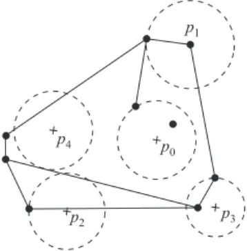
Ruppert [Ruppert, 1994] proposed a local feature size function (see Figure2.12) for a flat complex and proved that it yields planar meshes within a constant factor of the optimal size. Shewchuk [Shewchuk, 1997] used the same measure to prove grading bounds for tetrahedralizations.

Definition 35 (local feature size) The local feature size of a point p relative to a flat k-complex F in Rn_{, denoted by} _lfs_F₍_p₎_{, is the radius of the smallest} _n-ball

centered at p that intersects two non-incident pieces of _F.

p₃ p₂

p₁

p₀ p₄

Figure 2.12: Local feature size at the disks centers pi,i= 0, ...,4, graphically

repre-sented by the respective radius.

Theorem 2 (1-Lipschitz [Ruppert, 1994]) Thelocal feature sizeis 1-Lipschitz. Proof. Then-ballB_{of radius}_r _{= lfs}_F₍_p_{) centered at}_p_{intersects two non-incident}

pieces of F, by definition of local feature size. The ball of radius r′ ₌ _r₊_k_q₋_p_k

centered at q containsB _{and thus intersects the same two disjoint pieces of} _F _as B

does. Hence

lfsF(q)≤r′ =r+kq−pk= lfsF(p) +kq−pk (2.1)

and, since the same analysis is valid forp in relation to q,

|lfsF(q)−lfsF(p)|

(48)

Figure 2.13: Level curves of the local feature size (right) for a manifold complex with 3 pieces (left).

The local feature size can be extended to manifold complexes by stating that it is the radius of the ball that intersects two non-incident pieces or that contains a whole (≥1)-piece. This new definition (see Figure 2.13 for an illustrative example) also leads to a 1-Lipschitz function.

A common definition of local feature size for curved geometries used in shape reconstruction is the distance to themedial axis. With this definition, Amenta and Bern [Amenta and Bern, 1998] proved that sample points S _⊂ F_{, from a smooth}

curve or surface F_{, spaced a constant factor of the local feature size, is guaranteed}

to be reconstructed to a homeomorphic simplicial complex. Since the reconstructed shape is a homeomorphic mesh for the unknown F_{, the sampling condition also}

guarantees the existence of a homeomorphic mesh to F_{. However, this condition is}

much stricter than necessary when F _{is known. Similarly to the previous definition,}

the distance to the medial axis is also 1-Lipschitz.

2.4 Conclusions

The main result of this chapter is the definition of manifold complex, together with its properties. Its definition as a collection of open sets makes all connected pieces to a piece to lie in its boundary. One could make an equivalent definition in terms of closed sets. Some intersection properties are lost in the definition as open sets since all pieces are disjoint.

(49)

Chapter 3 Delaunay refinement

3.1 Basic concepts

3.1.1 Simplicial complex

Definition 36 (simplicial k-complex) A simplicialk-complex is amanifoldk-complex

or, more specifically, a flat k-complex where all n-pieces are open n-simplices, n = 0,1, ..., k, and all open j-simplicial facets of a n-simplex are in the complex, j = 0,1, ..., n.

n= 2 n= 1 n= 0

Figure 3.1: Example of a simplicial 2-complex (left) decomposed into its n -dimensional pieces.

Usually asimplicial k-complexis defined as a collection K of closedn-simplices,

n = 0,1, ..., k, where

1. every facet of a simplex in _K is also in_K;

2. a nonempty intersection of any two simplices inK is a facet of each of them.

In this text the definition as a collection of openn-simplices was employed to treat a simplicial k-complex as a natural special case of a manifold k-complex. Hence, a simplicial k-complex from a mesh generator must be an approximate partition of a manifold k-complex, or a finer partition of a flatk-complex.

3.1.2 Delaunay

In 1934, Boris Delaunay [Delaunay, 1934] introduced a condition for simplicial com-plexes that leaded to many interesting properties. It asserts that no vertices lie

(50)

inside a circumscribed ball of any element in the simplicial complex, as shown in Figure 3.2, known as the empty ball property. This is the basis of the Delaunay refinement and will be defined next under several aspects.

Figure 3.2: Example of a Delaunay triangulation (left) and a non Delaunay trian-gulation (right) for the same set of vertices.

Definition 37 (Delaunay simplicial complex [Delaunay, 1934]) A simplicial complex _S is Delaunay iff there exists an open circumscribed ball for every simplex

S_{∈ S} _{that contains no vertices.}

Definition 38 (strongly Delaunay simplicial complex) A simplicial complex

S is strongly Delaunay iff there exists a closed circumscribed ball for every simplex

S_{∈ S} _{that contains no vertices other than the vertices of} S_.

A Delaunay simplicial complex always exists for a set of points in Rn_{, but it is}

not unique when more than n+ 1 points lie in a common closed n-ball. In turns, a strongly Delaunay simplicial complex does not exist when more than n+ 1 points in Rn _{lie in a common} _closed_{n-ball, but it is always unique.}

3.1.3 Voronoi

In 1908 Georgy Voronoi [Voronoi, 1908] introduced the concept of partitioning a set into closest points to each point of a set.

Definition 39 (Voronoi cell) A Voronoi cell V _{of a point} _p _∈ S _⊂Rn _{is the set}

of all points that are closer to p than to any other point in S_, _i.e. V ₌ V_p ₌ _{_x _∈ Rn _{| k}_x₋_p_k_<_k_x₋_q_k_, _∀_q_∈S_{, q}₆₌_p_}_.

Definition 40 (Voronoi flat complex) The Voronoi flat complex of a point set

S _⊂ Rn _{is a} _flat _n-complex _{that contains the} _{Voronoi cells} _{of all elements in} _S _as

n-flat manifolds and their boundary partitioned into lower dimensional flat mani-folds.

TheVoronoi flat complex_VPof a point setP∈Rnis commonly known as Voronoi

diagram. It is closely related to a Delaunay simplicial complex of P_{, as shown in}

(51)

3.1. BASIC CONCEPTS ₄₇

Figure 3.3: Voronoi diagramand Delaunay triangulationfor the same set of points.

a(n−1)-flat. Conversely, every (n−1)-flat inV is equidistant to two distinct points in P_{. Following the sequence, every} _k_{-flat in} _V _{is equidistant to at least} _n₋_k_{+ 1}

points inP_,_k_{= 0}_,₁_{, ..., n}_{. (More than two distinct points can lie in the boundary of}

the same (>1)-ball. Hence the limit of n−k+ 1 points is obviously tight iff every point in a k-flat is equidistant to exactlyn₋k+ 1.)

Definition 41 (fully Delaunay simplicial complex) Let_Dbe a simplicial com-plex andV be the Voronoi flat complex of the vertices inD. ThenDis fully Delaunay iff it is Delaunay and every k-piece in_V is equidistant to exactly n₋k+ 1 vertices in _D.

Every n-simplex of a fully Delaunay simplicial complex _D is uniquely related to a vertex of the Voronoi flat complex VP of P because the set of points closest to n+ 1 affinely independent points inRn_{is a single point. Analogously, every (}_n₋_k

)-simplex in _D is uniquely related to ak-piece in_V. So there is a duality relationship between Voronoi flat complexes and Delaunay simplicial complexes.

Theorem 3 ([Watson, 1981]) Let P _∈ Rd _{be a set of points. If a subset} A _of

n+ 2, points in P _{lie in a common} ₍_n ₋₁₎_{-hypersphere, where} _{n < d}_{, then there}

exists a subset B _of _n_{+ 3} _{points in} P _{that lie in a common} _n_{-hypersphere.}

Proof. Since a (n₋1)-hypersphere is a cross-section of an n-hypersphere, any point added to A _{will lie in a common} _n_{-hypersphere with} A_.

Corollary 1 A simplicial complex is fully Delaunay iff it is strongly Delaunay.

(52)

Theorem 4 (strongly Delaunay) A simplicial complex _D in Rd _is _strongly

De-launay iff the sub-collection of n-simplices in _D is strongly Delaunay, for a single arbitrary n.

Proof. By definition, all n-simplices, for a givenn, in a Delaunay simplicial com-plex have the empty ball property. To prove the converse implication, consider the Voronoi flat complexV for the vertex set of D. If the simplicial complex is strongly Delaunay, every vertex of _V is uniquely related to a d-simplex of _D. Suppose, by contradiction, a (d₋1)-simplex not in _D has the empty ball property. Then grow this ball until another vertex is met. The resulting d-simplex must be uniquely related to a vertex in _V, which cannot be true since it is not in _D. By induction, every k-piece of _V is uniquely related to a (d₋k)-simplex of_D. Then grow this ball until another vertex is met. The resulting (d−k)-simplex must be uniquely related to a k-piece in _V, which cannot be true since it is not in_D.

Shewchuk [Shewchuk, 1997] has proven in his thesis the strongly Delaunay the-orem for n= 2 using a different approach.

3.1.4 Conforming Delaunay

Definition 42 (conforming Delaunay simplicial complex) A simplicial com-plex_S is conforming Delaunay to a flat complex_F iff _S is Delaunay and each piece of F is a union of pieces in S.

In a conforming Delaunay simplicial complex of _F, the vertices of _F are aug-mented by additional vertices, called Steiner points, so that its simplices conforms_F and are Delaunay. Edelsbrunner and Tan [Edelsbrunner and Tan, 1993] show that any flat 2-complex _F can be triangulated with no more than O(m2_n_{) augmenting} vertices, where m is the number of edges in _F, and n is the number of vertices in

F.

3.1.5 Constrained Delaunay

Definition 43 (visible) A point p _∈ Rd _{is visible from another point} _q _∈ Rd _in

respect to a (d₋1)-piece S _{contained in a} _(d₋_1)-flat F _{iff either the line segment}

pq does not intersect the closure of S_{, or} _pq _{lies in}F_.

Definition 44 (constrained Delaunay simplicial complex) Asimplicial com-plex _S is constrained Delaunay upon a flat complex _F iff it has no vertices not in

F, each piece of F is a union of pieces inS, and there exists anopen circumscribed ball for every simplex S_{∈ S} _{that contains no vertices} _visible_from S _{in respect to} _F_.

Unlike conforming Delaunay simplicial complexes, constrained Delaunay sim-plicial complexes do not allow any augmenting vertex. Because of this, some flat

Delaunay refinement for curved complexes