Rainer Ronnie Pereira Couto
Compress˜
ao Adaptativa de Arquivos HTML em
Ambientes de Comunica¸
c˜
ao Sem Fio
Disserta¸c˜ao apresentada ao Curso de P´os-Gradua¸c˜ao em Ciˆencia da Computa¸c˜ao da Universidade Federal de Minas Gerais, como requisito parcial para a obten¸c˜ao do grau de Mestre em Ciˆencia da Computa¸c˜ao.
Acknowledgements
As the popular saying goes: “Behind a every great man there is always a great woman”. Well, I’m not that great yet, but I already have the love of four great women to inspire me: my mother, my two sisters and my niece. There are no words to describe how important you are in my life. I love you more than you can imagine.
It would be impossible to get here without the help of my friends. They were my strength when I wanted to give everything up, so this work is dedicated to all of them, specially to:
• Ricardo A. Rabelo, it is an honor to have you as my friend and to work with you.
• Linnyer Beatrys Ruiz, my “third” sister. You were always a bright light in my path during all these years. Thank you for your company and peaceful words.
• Fernanda P. Franciscani, my friend of work, laughs and studies. I wish I could have someone as special as you in whatever place God takes me to work.
• Ana Paula Silva, thank you for being so loving and so tender.
• Renan Cunha, Wagner Freitas, Vin´ıcius Rosalen, F´atima and Lidiane Vogel. Thank you for the companionship during those hot afternoons inside SIAM lab.
• Many thanks also to Cl´audia, Camila, M´arcia and Luciana. Your friendship along these past 10 years means a lot to me.
• Antonio A. Loureiro, my advisor and my “academic father”. Thank you for all the words, patience, time, and knowledge you dedicated me. My only wish is to make you proud.
Abstract
Resumo
Contents
List of Figures vi
List of Tables viii
1 Introduction 1
2 Related work 6
3 Compression methods 10
3.1 Compression Algorithms . . . 12
3.2 Performance Evaluation . . . 15
3.2.1 Calgary and Canterbury Corpus Collections . . . 16
3.2.2 HTML Files . . . 22
3.2.3 XML Files . . . 26
4 Adaptive model 37 5 Experiments 45 5.1 Communication protocols . . . 45
5.1.1 IEEE 802.11 . . . 45
5.1.2 Bluetooth . . . 46
5.2 Scenarios . . . 47
5.3 Results . . . 49
5.3.1 An analytical view . . . 54
5.4 Simulations . . . 55
6 Proxy experiments 59 6.1 HTTP Trace . . . 61
6.2 RabbIT 2 Implementation . . . 65
7 Conclusion 69
7.1 Future Works . . . 69
List of Figures
1.1 Example of a typical middleware architecture used for adaptation in wireless
environments. . . 3
1.2 S is a Web server and Ci’s are the requesting clients. . . 4
3.1 Compressed sizes of Calgary Corpus files. . . 18
3.2 Compression and decompression times versus Compression Ratio (Calgary Corpus). . . 19
3.3 Compression and decompression times for the Calgary collection. . . 20
3.4 Compressed sizes of Canterbury Corpus files. . . 21
3.5 Compression and Decompression times versus Compression Ratio (Canter-bury Corpus). . . 22
3.6 Compression and decompression times for Canterbury Corpus collection. . 23
3.7 Accumulated distribution for original and compressed files in the HTML collection. . . 24
3.8 Compression time versus file size (HTML Collection). . . 26
3.9 Decompression time versus file size (HTML Collection). . . 27
3.10 Compression and Decompression times versus Compression Ratio (HTML Collection). . . 28
3.11 Compression and decompression times for HTML files and gzip-6 algorithm. 28 3.12 File size distribution of XML files. . . 30
3.13 Compression and Decompression times versus Compression Ratio (XML Collection). . . 31
3.14 File size distribution of XML files. . . 31
3.15 Compression and Decompression times versus Compression Ratio (XML Collection). . . 32
3.16 Compression and decompression times for XML medical Collection. . . 33
3.17 Compression and decompression times for XML Sigmod Collection. . . 34
5.1 File size versus decompression time for files smaller than 15 Kbytes. . . 48
5.2 Scenario of 802.11 experiments. . . 48
5.3 Response time for adaptive, compressed and not compressed models. . . . 50
5.4 Percentual gain of adaptive model over compressed and not compressed models. . . 51
5.5 Accumulated consumed energy of adaptive, compressed and not compressed models . . . 51
5.6 Response time for adaptive, compression and not compression models using bandwidth of 2 Mbps and processor speed of 66 MHz. . . 52
5.7 Response time for adaptive, compression and not compression models using bandwidth of 1 Mbps and processor speed of 33 MHz. . . 53
5.8 Response time for the Bluetooth protocol. . . 53
5.9 Response time as a function of file size and bandwidth. . . 54
5.10 Graphical view of compression of the analytical model. . . 55
5.11 Comparison of adaptive, compression and not compression models (1 client). 57 5.12 Performance of adaptive over not compression model with varying energy weight. . . 58
5.13 Comparison of the adaptive and not compression models in Bluetooth envi-ronment. . . 58
6.1 Proxy system. . . 60
6.2 Distribution of Content Type. . . 62
6.3 Session view of the trace. . . 63
6.4 User1 Trace. . . 64
6.5 Page rank by access (all users). . . 64
6.6 Page rank by access (User1). . . 65
6.7 File size distribution (all users). . . 66
6.8 File size distribution (User1). . . 66
List of Tables
3.1 Description of the compression algorithms tested. . . 15
3.2 Description of Calgary Corpus files. . . 16
3.3 Description of Canterbury Corpus files. . . 17
3.4 Compressed size of Calgary Corpus files. . . 35
3.5 Compressed size of Canterbury Corpus files. . . 36
4.1 Approximate compression ratio as a function of compression method and original size for HTML files. . . 42
4.2 Decompression time constant as a function of compression method. . . 43
Chapter 1
Introduction
The development of mobile computing technologies has increased rapidly during the last decade. Mobile devices and wireless communication are already present in our daily activi-ties such as when using devices like cellular phones, Personal Digital Assistants (PDAs) and notebooks, or interacting with embedded systems and sensors. Nonetheless, the advances in wireless and mobile world have not kept pace with their counterparts in wired networks due to restrictions such as less processing power, limited transmission range, complex man-agement of energy consumption, limited size and low bandwidth availability [1]. Processing power in mobile devices is notably inferior when compared to a common desktop computer. Both transmission range and energy consumption are regulated by communication proto-cols. For instance, Bluetooth devices are often smaller, have lower transmission range and less energy consumption than devices designed for a IEEE 802.11 [2] environment.
bandwidth as it depends on the user’s physical location, higher bit error ratio and others features of this environment. Besides, they also have to deal with specific problems such as seamless communication, hidden node problems, disconnection, etc.
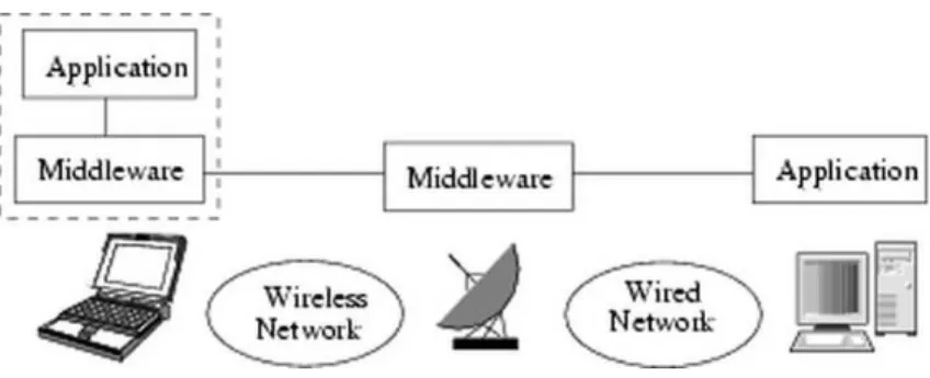
These restrictions present real challenges when developing applications for wireless en-vironments. One solution to overcome these problems isadaptability [1, 3, 4]. Adaptation consist in altering or adjusting the application’s behavior according to its awareness of the environment. Adaptation can be done in several ways depending on the application, the environment, user or systems goals and communicating devices. It is more effective when it occurs dynamically, that is, when the adaptation process “polls” the environment and decides which action should be taken during execution time. The aim is to save or at least minimize consumption of scarce resources, such as energy and bandwidth, or to optimize properties that are more visible to users – like response time and data quality. Exam-ples of adaptability are 1) caching emails or Web pages on the mobile device itself so the user can access their content even if a wireless connection is not available at the moment, 2) adaptive power control that enables devices to transmit data in a lower transmission power when they are closer to base stations or other communication points and 3) adaptive channel allocation, which enables devices to select among several channels the one without interference of other signals [3]. The adaptation process may be located in different places such as in the application, in the system, or in a specific middleware. The middleware approach has the advantage of software reuse since already existing applications, systems and protocols need little or no modification at all. Usually, a middleware designed for wireless environment would be divided in two components – one in the device and another one in a point between the device and its peer on the wired network (for instance, the base station). An example of middleware architecture is shown in Figure 1.1.
Figure 1.1: Example of a typical middleware architecture used for adaptation in wireless environments.
over the wireless channel, video quality can be altered to fit screen size, frequently accessed data can be cached next to users, location dependent data can be served to users inside a specific area, etc.
Most applications for handheld device are developed for PalmOS and Windows op-erating systems (e.g., PocketPC, Windows CE). In both cases, these opop-erating systems mimic the traditional interaction concepts of desktop computers such as icons, windows, and menus. As computers and the Internet become more popular, the acceptance of this interface concept also increases. In fact the World Wide Web, probably the most pop-ular Internet application, uses the direct manipulation interface based on this concept. Thus, it is natural to assume that the WWW will become a popular application for mobile environments as well.
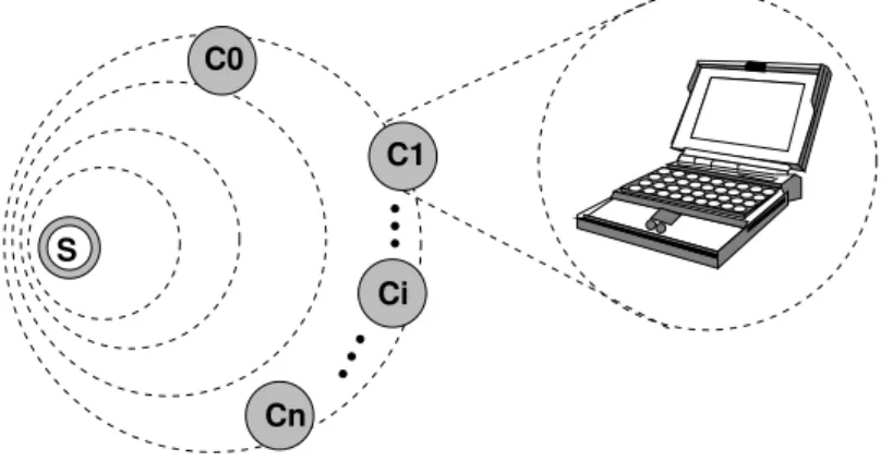
hand, compressed files need to be compressed and decompressed which may increase total response time and may consume more energy than uncompressed transmissions. Suppose the following scenario: a Web server accessed by different clients through a wireless channel (figure 1.2). As each device has its own features and these features vary highly in this het-erogeneous environment, the decision to compress one file is not a simple task and should be done carefully by the server. For some application/device combination compression can be worthwhile, while the same application in a different device might perform better with no compression at all.
S
C1
Ci
Cn C0
Figure 1.2: S is a Web server and Ci’s are the requesting clients.
This work studies the conditions in which compression should happen and how it should be done when dealing with HTML file transmissions. The focus is on HTML files, but the technique developed here could be extended to images and videos as well. So, this work intends to:
1. study which compression method is more adequate to be used in mobile devices for HTML file transmission;
2. propose an adaptive model that predicts when compression of HTML files should happen;
Chapter 2
Related work
According to [3],adaptability is the system ability to configure itself dynamically in order to take advantage of the environment it is inserted in. It is assumed that the system has means to get information about environmental conditions. When one of these conditions changes, an adaptation process should take place so the better solution/answer is achieved. Although not restricted to the wireless world, adaptation fits better to this environment due to its intrinsic characteristics.
Adapting an application means changing its normal behavior in any of its functional modules, going from higher layers such as user interface to lower layers in the communi-cation procedures. This last module – communicommuni-cation – plays a key role on distributed applications and it is one of the most affected modules when a change in the environmen-tal conditions occurs. In order to react to these changes, adaptation techniques may be applied/inserted in any of the several layers that compose thenetwork access stack. Next, some adaptation processes applied to wireless and wired network protocols that attempt to improve Web-like access experience through compression, which is the object-study application of this work, are reviewed.
Web-proxy – TranSend – and its evaluation, their work has the merit to argue in favor of proxy architecture as being the most effective and extensible technique to handle client and server heterogeneity. The programming model presented is based onworkers, a set of task-specific elements specialized in operations such as transformation (distillation, filter-ing, etc.), aggregation (collecting and collating data from various sources), caching (both original and transformed content), and customization (change data to user specific needs and preferences).
Housel, Samaras, and Lindquist [9] presented WebExpress, a split-proxy design trans-parent to clients and servers, which intercepts HTTP data streams and performs several optimizations, including file-caching, forms differencing, protocol reduction, and elimina-tion of redundant HTTP header transmission.
Steinberg and Pasquale [6] proposed a Web middleware architecture – WSC (Web Stream Customizer) – for mobile devices that allows users to customize their view of the Web for optimal interaction. Like WebExpress, WSC explores the proxies capabilities of HTTP to adapt the point-to-point traffic along the client-server path. It uses a simple adaptive model based solely on network characteristics to compress text data (lossless compression) and image data (lossy compression).
good results for transmission of large amounts of data, which is not the case for mobile HTTP browsing.
Mogul et al. [5] used data compression and delta-encoding to minimize the amount of data transmitted and response time. Delta-encoding is a technique to update cached documents by sending only the information about portions of the page which have changed. They propose specific extensions to the HTTP protocol to achieve these goals. [12, 13, 14] try to reduce the amount of data transmitted to mobile devices by extracting relevant information of HTML pages. Their goal is to expose the mobile users, whose devices have screen size limitations, to a minimum but relevant set of information each time it performs a new request. The techniques applied by them involve removing HTML and data components such as pop-ups, images and extraneous links, and text summarization, which means using HTML structure to extract the most relevant data.
On the other hand, there are several proposals that focus on lower layer modifications to improve response time or energy consumption of mobile devices.
Jung and Burleson demonstrated in [15] the advantages of using compression through VLSI (very-large-scale integration) hardware components to increase effective bandwidth in wireless communication systems. They modelled and simulated a real-time, low-area, and low-power VLSI lossless data compressor based on the first Lempel-Ziv algorithm [16] to improve the performance of wireless local area networks. Simulations were made with IEEE 802.11 protocol in which only the payload of MAC layer packets were compressed before transmission. The results showed that the architecture can achieve an average compression rate of 50 Mbps consuming approximately 70mW in 1.2u CMOS, which is an ideal scenario for WLAN use. This means this compression scheme can improve throughput and delay of a network while minimizing average power consumption.
be-tween the Power-Saving Mode (PSM) of IEEE 802.11 and the performance of TCP trans-fers under typical Web browsing workloads. It is proposed another PSM that dynamically adapts to network activity and simultaneously reduces energy consumption and response time.
Chapter 3
Compression methods
Over the past years, mass storage systems and network transfer rates have increased reg-ularly. At the same time though the demand for these items has grown proportionally or even higher as each day more and more data are created and this huge volume of data needs to be handled efficiently – storing, recovering, and transmitting it. In many cases, the solution to cope with such an amount of information is to use compression. The ad-vantage is twofold: it provides both lower transmission times and less storage space, thus satisfying the needs of users and information providers.
Compression methods can be divided in two main categories: lossless (mainly used for text compression) and lossy (used for general data compression). Lossless compression involves changing the representation of a file, yet the original copy can be reconstructed exactly from the compressed representation [19]. Losslesscompression is a specific branch of the more generallossycompression methods, which are methods that tolerate the insertion of noise or small changes during the reconstruction of the original data. They are usually used in images and sound compression or any other digital data that is an approximation of an analog waveform.
that this limit is determined by the statistical nature of the information source and called it theentropy rate- denoted byH. He then proved mathematically that it is impossible to compress the information source in a lossless manner with compression rate higher than
H.
Shannon also developed the theory of lossy data compression, also known as rate-distortion theory. In lossy data compression, the decompressed data does not have to be exactly the same as the original data, that is, some amount of distortion, D, is tolerated. Shannon showed that, for a given source (with all its statistical properties previously known) and a given distortion measure there is a functionR(D), called the rate-distortion function, that gives the best possible compression rate for that source. The theory says that ifD is the tolerable amount of distortion, then R(D) is the best possible compression rate. If the allowed distortion D is set to 0, then compression becomes lossless and the best compression rate R(0) is equal to the entropy H (for a finite alphabet source). The conclusion is thatlosslesscompression (D= 0) is a specialization of the more general lossy
compression (D≥0).
Lossless data compression theory and rate-distortion theory are known collectively as
source coding theory. Source coding theory sets fundamental limits on the performance of all data compression algorithms. The theory in itself does not specify exactly how to design and implement these algorithms. It does, however, provide some hints and guidelines on how to achieve optimal performance.
3.1
Compression Algorithms
Two strategies are used to design text compression algorithms: statistical or symbolwise
methods anddictionarymethods. Symbolwisemethods work by estimating the probabilities of symbols (often characters) occurrences, and then coding one symbol at a time using shorter codewords for the most likely symbols. Dictionary methods achieve compression by replacing words and other fragments of text with an index to an entry in a dictionary [19].
The key distinction between symbolwise and dictionary methods is that symbolwise methods generally base the coding of a symbol in the context in which it occurs, whereas dictionary methods group symbols together, creating a kind of implicit context. In the first scheme, fixed-length blocks of bits are encoded by different codewords; in the second one, variable-length segments of text are encoded. This second strategy often provides better compression ratios. Hybrid schemes are also possible, in which a group of symbols is coded together and the coding is based on the context in which the groups occurs. This does not necessarily provide better compression but it can improve speed of compression.
Many compression methods have been invented and reinvented over the years. One of the earliest and best-known methods of text compression for computer storage and telecommunications is Huffman coding. Huffman coding assigns an output code to each symbol, with the output codes being as short as 1 bit or considerably longer than the input symbols, strictly depending on their probabilities. The optimal number of bits to be used for each symbol is the log2(1p), where p is the probability of a given character inside the text being compressed. Moreover, Huffman algorithm uses the notion ofprefix
a longer compressed data as each code has influence in the other ones. The second problem is that the probability function generally is not known from the beginning, demanding an extra pass through the input file to estimate it.
Despite its problems, Huffman code was regarded as one of the best compression meth-ods from its first publishment (in the early 1950s) until the late 1970s, when adaptive compressionallowed the development of more efficient compressors. Adaptive compression is a kind of dynamic coding where the input is compressed relative to a model that is constructed from the text that has just been coded. Both the encoder and decoder start with their statistical model in the same state. Each of them process a single character at a time, and update their models after the character is read in. This technique is able to encode an input file in one single pass over it and it is able to compress effectively a wide variety of inputs rather than being fine-tuned for one particular type of data. Ziv-Lempel method and arithmetic coding are examples of adaptive compression.
Ziv-Lempel methods are adaptive compression techniques that have good compression yet are generally very fast and do not require large amounts of memory. Ziv-Lempel
algorithms compress by building a dictionary of previously seen strings, grouping characters of varying lengths. The original algorithm did not use probabilities - strings were either in the dictionary or not, and to all strings the same probability is given. Some variants of this method, such asgzip, use probabilities to achieve better performance. The algorithm can be described as follow: given a specific position in a file, look for a previous position in the file that matches the longest string starting at the current position; output a code indicating the previous position; move the current header position over the string coded and start again. Ziv-Lempel algorithms were described in two main papers published in 1977 [16] and 1978 [21] and are often referred to as LZ77 and LZ78. These two version differ in how far back the match can occur: LZ77 uses the idea of a sliding window; LZ78 uses only the dictionary. Some well known variants of LZ77 aregzipand zip, whereas Unix
LZ78, creating the so called LZW algorithm, one of the most popular compressors today, used in formats such as GIF and TIFF and is also part of PostScript Level 21.
Arithmetic coding is an enabling technology that makes a whole class of adaptive com-pression schemes feasible, rather than a comcom-pression method of its own. This technique has made it possible to improve compression ratios, though compression and decompres-sion processes are slower - several multiplications and dividecompres-sions for each symbol are needed - and more memory must be allocated during processing. Arithmetic coding completely bypasses the idea of replacing an input symbol with a specific code. Instead, the idea is to represent the input string by one floating-point number n in the range [0..1]. In order to construct the output number, the symbols being encoded have to have a set of probabilities assigned to them. Then, to each symbol is assigned an interval with size proportional to its respective probability. The algorithm works as follow: Starting with the interval [0..1], the current symbol determines which subinterval of the current interval is to be considered. The subinterval from the coded symbol is then taken as the interval for the next symbol. The output is the interval of the last symbol. Implementations write bits of this interval sequence as soon as they are certain. The longer the input string is, the more numbers after the floating point are needed to represent it.
Some of the best compression methods available today are variants of a technique called
prediction by partial matching(PPM), which was developed in the early 1980s. PPM relies on arithmetic coding to obtain good compression performance. Since then there has been little advance in the amount of compression that can be achieved, other than some fine-tuning of the basic methods. On the other hand, many techniques have been discovered that can improve the speed or memory requirements of compression methods. One exception is Burrows-Wheeler Transform or BWT. BWT method was discovered recently by Burrows and Wheeler in [24] and it is implemented inbzip, one of the best text compressor available currently. It can get ratio performance close to PPM, but runs significantly faster. The
1
BWT is an algorithm that takes a block of data and rearranges it using a sorting algorithm. The resulting output block contains exactly the same data elements that it started with differing only in their ordering. The transformation is reversible, meaning the original ordering of the data elements can be restored with no loss of fidelity. At last, the sorted block is passed to a entropy encoder, typically Huffman or arithmetic encoder.
3.2
Performance Evaluation
This section presents the results of different compression algorithms applied to different data sets. The goal here is to analyze which compression methods are suitable to be used on wireless transmissions of Web files. Four different collections are used in these experiments. The Calgary and Canterbury Collections are well known data sets used to analyze performance of compression algorithms. In order to have a more realistic measure, it was formed a new collection by crawling 9513 files from the Web. For the sake of comparison, it was also measured compression performance for XML collections. The first XML collection is the National Library of Medicine public collection [25]. The second one was formed by all XML files hosted in the Sigmod [26] Web site.
Table 3.1 summarizes all different compression algorithms tested.
Table 3.1: Description of the compression algorithms tested.
Algorithm Description
LZW The original LZW algorithm
COMP1 Arithmetic coding
COMP2 Improved Arithmetic coding
HUFF Huffman coding
LZ77 The original LZ77 algorithm
LZARI Improved LZ77
LZSS Improved LZ77
PPMC PPM compressor
GZIP LZSS variant
BZIP2 Burrows-Wheeler algorithm
3.2.1
Calgary and Canterbury Corpus Collections
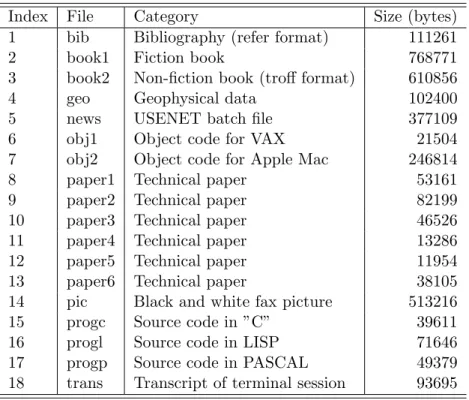
The Calgary Corpus collection was developed in 1987 by Ian Witten, Timothy Bell and John Cleary for their research paper on text compression modeling [27] at University of Calgary, Canada. During the 1990s it became the standard benchmark for lossless compression evaluation. The collection is now rather dated but it is still reasonably reliable. Table 3.2 has the details.
Table 3.2: Description of Calgary Corpus files.
Index File Category Size (bytes)
1 bib Bibliography (refer format) 111261
2 book1 Fiction book 768771
3 book2 Non-fiction book (troff format) 610856
4 geo Geophysical data 102400
5 news USENET batch file 377109
6 obj1 Object code for VAX 21504
7 obj2 Object code for Apple Mac 246814
8 paper1 Technical paper 53161
9 paper2 Technical paper 82199
10 paper3 Technical paper 46526
11 paper4 Technical paper 13286
12 paper5 Technical paper 11954
13 paper6 Technical paper 38105
14 pic Black and white fax picture 513216
15 progc Source code in ”C” 39611
16 progl Source code in LISP 71646
17 progp Source code in PASCAL 49379
18 trans Transcript of terminal session 93695
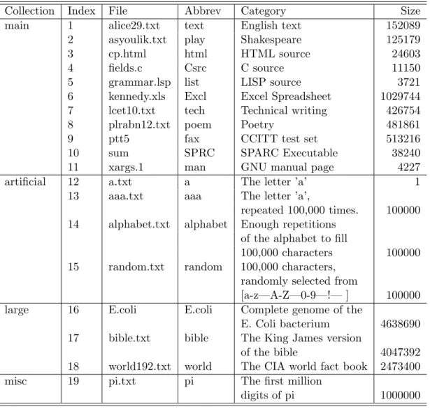
because of large amounts of white space in the picture represented by long runs of zeros. Developed in 1997, the Canterbury Corpus is an improved replacement for the Calgary Corpus. Today, this collection is the main benchmark for comparing compression methods. The main files in the collection are listed on table 3.3.
Table 3.3: Description of Canterbury Corpus files.
Collection Index File Abbrev Category Size
main 1 alice29.txt text English text 152089
2 asyoulik.txt play Shakespeare 125179
3 cp.html html HTML source 24603
4 fields.c Csrc C source 11150
5 grammar.lsp list LISP source 3721
6 kennedy.xls Excl Excel Spreadsheet 1029744
7 lcet10.txt tech Technical writing 426754
8 plrabn12.txt poem Poetry 481861
9 ptt5 fax CCITT test set 513216
10 sum SPRC SPARC Executable 38240
11 xargs.1 man GNU manual page 4227
artificial 12 a.txt a The letter ’a’ 1
13 aaa.txt aaa The letter ’a’,
repeated 100,000 times. 100000
14 alphabet.txt alphabet Enough repetitions
of the alphabet to fill
100,000 characters 100000
15 random.txt random 100,000 characters,
randomly selected from
[a-z—A-Z—0-9—!— ] 100000
large 16 E.coli E.coli Complete genome of the
E. Coli bacterium 4638690
17 bible.txt bible The King James version
of the bible 4047392
18 world192.txt world The CIA world fact book 2473400
misc 19 pi.txt pi The first million
digits of pi 1000000
performance – files containing little or no repetition (e.g. random.txt), files containing large amounts of repetition (e.g. alphabet.txt), or very small files (e.g. a.txt). The Large Corpus is a collection of relatively large files. While most compression methods can be evaluated satisfactorily on smaller files, some require very large amounts of data to get good compression, and some are so fast that the larger size makes speed measurement more reliable. The Miscellaneous Corpus is a collection of “miscellaneous” files that is designed to be added to by researchers and others wishing to publish compression results using their own files.
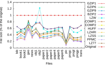
Figure 3.1 plots the compressed ratios of Calgary Corpus files. Table 3.4 at the end of the chapter shows each point individually. As it can seen, PPM, arithmetic (COMP2) and bzip2 methods had the best performances, followed by gzip and other LZ-like methods. Huffman had the worst performance. This is an expected behavior, as explained in Section 3.1. 0 0.2 0.4 0.6 0.8 1 1.2 1.4 trans progp progl progc pic paper6 paper5 paper4 paper3 paper2 paper1 obj2 obj1 news geo book2 book1 bib
File size (% of the original)
Files GZIP1 GZIP6 GZIP9 BZIP2 LZW COMP1 COMP2 HUFF LZARI LZSS PPMC LZ77 Original
Figure 3.1: Compressed sizes of Calgary Corpus files.
time/compression ratio tradeoff should be used. Figure 3.2(a) plots tradeoff between av-erage compression time and avav-erage compression ratio for all Calgary Corpus files and for each compression algorithm analyzed. Figure 3.2(b) does the same analysis for average decompression time. 0.01 0.1 1 10 100
0 0.2 0.4 0.6 0.8 1
Compression time (s)
Compression ratio LZW COMP1 COMP2 HUFF LZ77 LZARI LZSS PPMC GZIP1 GZIP6 GZIP9 BZIP2 (a) Compression 0.01 0.1 1 10
0 0.2 0.4 0.6 0.8 1
Decompression time (s)
Compression ratio LZW COMP1 COMP2 HUFF LZ77 LZARI LZSS PPMC GZIP1 GZIP6 GZIP9 BZIP2 (b) Decompression
Figure 3.2: Compression and decompression times versus Compression Ratio (Calgary Corpus).
best choice. Although PPM and BZIP2 yields good compression rates, their compression and decompression times are almost one order of magnitude higher than gzip.
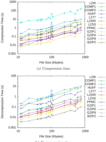
It is important to notice that compression and decompression times grow proportionally to file size (figures 3.3(a) and 3.3(b)). This is an important aspect of compression once it can be used to predict, with certain precision, how long it will take to compress or decompress a file. To make such a prediction, one must perform a linear regression on the values obtained and create a formula that calculates time according to each file size. This subject will be explored again on chapter 4.
0.001 0.01 0.1 1 10 100 1000
10 100 1000
Compression Time (s)
File Size (Kbytes)
LZW COMP1 COMP2 HUFF LZ77 LZARI LZSS PPMC GZIP1 GZIP6 GZIP9 BZIP2
(a) Compression time.
0.001 0.01 0.1 1 10 100
10 100 1000
Decompression Time (s)
File Size (Kbytes)
LZW COMP1 COMP2 HUFF LZ77 LZARI LZSS PPMC GZIP1 GZIP6 GZIP9 BZIP2
(b) Decompression time.
Figure 3.4 show compression ratios for Canterbury Corpus files. Again PPM, arithmetic and bzip2 methods had the best global performance. Three files presented an anomalous behavior due to their natural properties: a, aaa and alphabet. They are either too small or have an enormous amount of repeated information. In both cases some algorithms may present unexpected behavior. As this is not the case for most files in Internet, these values can be disregarded. Table 3.5 at the end of the chapter shows all values individually.
0 0.2 0.4 0.6 0.8 1 1.2 pi world bible E.coli man SPRC fax poem tech Excl list Csrc html play text random alphabet aaa a
File size (% of the original)
Files GZIP1 GZIP6 GZIP9 BZIP2 LZW COMP1 COMP2 HUFF LZARI LZSS PPMC Original
Figure 3.4: Compressed sizes of Canterbury Corpus files.
reasonable to assume that this is the mean compressing ratio of each algorithm. 0.001 0.01 0.1 1 10 100
0.001 0.01 0.1 1 10 100
Compression time (s)
Compression ratio LZW COMP1 COMP2 HUFF LZARI LZSS PPMC GZIP1 GZIP6 GZIP9 BZIP2 (a) Compression 0.001 0.01 0.1 1 10 100
0.001 0.01 0.1 1 10 100
Decompression time (s)
Compression ratio LZW COMP1 COMP2 HUFF LZARI LZSS PPMC GZIP1 GZIP6 GZIP9 BZIP2 (b) Decompression
Figure 3.5: Compression and Decompression times versus Compression Ratio (Canterbury Corpus).
Figures 3.6(a) and 3.6(b) plot compression and decompression times versus file size. As Canterbury Corpus has irregular files, the proportion of both compression and decompres-sion times versus file size are affected by them. However, it is still possible to determine such proportion by just ignoring or amortizing the effects of these outliers.
3.2.2
HTML Files
0.001 0.01 0.1 1 10 100 1 10 100 1000 10000
100000 1e+06 1e+07
Compression Time (s)
File Size (Kbytes)
LZW COMP1 COMP2 HUFF LZARI LZSS PPMC GZIP1 GZIP6 GZIP9 BZIP2
(a) Compression time.
0.001 0.01 0.1 1 10 100 1 10 100 1000 10000
100000 1e+06 1e+07
Decompression Time (s)
File Size (Kbytes)
LZW COMP1 COMP2 HUFF LZARI LZSS PPMC GZIP1 GZIP6 GZIP9 BZIP2
(b) Decompression time.
Figure 3.6: Compression and decompression times for Canterbury Corpus collection.
and programming language code. From now on, all these files will be referred as HTML files. HTML files account for more than 97% of all documents found in the Internet that are considered as textual information [28]. HTML files are exclusively textual, since their contents consist of formatting tags and the text itself. This kind of language compensates easiness of human reading with extremely verbose and large documents.
the previous section gave us an idea of how these metrics are for text collections. As it will be seen now, HTML have a similar behavior.
Figure 3.7(a) gives the accumulated size distribution of all files in the collection and the amount of files in each range. As it can be seen, there is a concentration of files in the range of 10-30Kbytes. Figure 3.7(b) represents accumulated compressed size distribution for all algorithms tested.
0 0.1 0.2 0.3 0.4 0.5 0.6 0.7 0.8 0.9 1 1.1
0.1 1 10 100 1000
0 500 1000 1500 2000 2500 Accumulated Distribution
Number of files
File size (kbytes) Distribution
No. of files
(a) Accumulated distribution of the original HTML files.
0 0.1 0.2 0.3 0.4 0.5 0.6 0.7 0.8 0.9 1 1.1
0.1 1 10 100 1000
Accumulated distribution
File size (kbytes)
GZIP1 GZIP6 GZIP9 BZIP2 LZW COMP1 COMP2 HUFF LZARI LZSS PPMC Original
(b) Accumulated distribution of compressed HTML files.
By doing the same experiments with this collection, the following results can be ob-served. Regarding small files (smaller than 5kbytes), PPM and arithmetic methods perform better than others. PPM, bzip2, arithmetic and gzip-9 methods achieve almost the same compression limit for larger files. Finally, although gzip-1 and gzip-6 can not compress as much as gzip-9, they compress and decompress faster than others, yielding a good time/ratio tradeoff. Figures 3.8(a) and 3.9(a) show compression and decompression times. The best way to visualize these results is plotting them using some kind of linear regres-sion of curve fitting. Although Bezier curves are not used to create a function definition for the data, this curve fitting method serves the purpose of giving an approximation of the function line as it would be obtained through linear regression. Figures 3.8(b) and 3.9(b) shows the curve fitting for all algorithms tested and make it easy to observe how the performance of each compression technique vary according to file size.
Figures 3.10(a) and 3.10(b) illustrate compression and decompression times versus com-pression ratio, respectively. Instead of a point representing the average of all measures taken, it was plotted lines representing time versus compression ratio for the several ratios obtained with each algorithm. This way it is possible to see how compression ratio and compression/decompression time are related. An algorithm with good time/ratio tradeoff would generate a line with points concentrated in the lower left corner of the graph.
BZIP2 0.01 0.1 1 10 100
0.1 1 10 100 1000
Compression Time (s)
File Size (Kbytes)
LZW COMP1 COMP2 HUFF LZARI LZSS PPMC GZIP1 GZIP6 GZIP9 0.001
(a) Compression time (all points).
BZIP2 0.01 0.1 1 10 100
0.1 1 10 100 1000
Compression Time (s)
File Size (Kbytes)
LZW COMP1 COMP2 HUFF LZARI LZSS PPMC GZIP1 GZIP6 GZIP9 0.001
(b) Compression time (using a smooth bezier curve to plot all points).
Figure 3.8: Compression time versus file size (HTML Collection).
3.2.3
XML Files
The XML specification defines a standard way to add markup points to documents con-taining structured information [29]. Structured information contains both content (words, pictures, etc.) and some indication of what role that the content plays. XML specifies neither semantics nor a tag set and it is not a markup language per se. XML is really a meta-language for describing markup languages. In other words, XML provides a facility to define tags and the structural relationships between them.
BZIP2 0.01 0.1 1 10 100
0.1 1 10 100 1000
Compression Time (s)
File Size (Kbytes)
LZW COMP1 COMP2 HUFF LZARI LZSS PPMC GZIP1 GZIP6 GZIP9 0.001
(a) Decompression time (all points).
BZIP2 0.01 0.1 1 10 100
0.1 1 10 100 1000
Compression Time (s)
File Size (Kbytes)
LZW COMP1 COMP2 HUFF LZARI LZSS PPMC GZIP1 GZIP6 GZIP9 0.001
(b) Decompression time (using a smooth bezier curve to plot all points).
Figure 3.9: Decompression time versus file size (HTML Collection).
BZIP2
0.01 0.1 1 10
0 0.2 0.4 0.6 0.8 1 1.2 1.4 1.6
Compression time (s)
Compression ratio LZW COMP1 COMP2 HUFF LZARI LZSS PPMC GZIP1 GZIP6 GZIP9 0.001 (a) Compression BZIP2 0.01 0.1 1 10
0 0.2 0.4 0.6 0.8 1 1.2 1.4 1.6
Uncompression time (s)
Compression ratio LZW COMP1 COMP2 HUFF LZARI LZSS PPMC GZIP1 GZIP6 GZIP9 0.001 (b) Decompression
Figure 3.10: Compression and Decompression times versus Compression Ratio (HTML Collection).
Decompression
0.01 0.1 1
0.1 1 10 100 1000
Compression Time (s)
File Size (Kbytes) Compression
0.001
Figure 3.11: Compression and decompression times for HTML files and gzip-6 algorithm.
Any file that follows the general markup rules can be a valid XML file. Most XML applications follow a more rigorous set of rules having their structure defined by aDocument Type Definition (DTD) or by a schema, which provides even more information about the content than a DTD.
As in HTML, XML substantially increases the size of data files over the size when the same data is represented in raw format. By using compression, the impact of this inherent inflation can be minimized. Compression of XML files can be greatly increased when the schema is available. The schema allows the XML tags to be encoded with high efficiency. In addition to providing high compression of tag data, knowledge of the schema allows the element data to be encoded efficiently. Because schemas supply the data type information, compression routines optimized for specific data types can be used, providing extremely high compression ratios. If a file does not conform to the expected schema, the data is safely encoded using high-performance general-purpose coders.
For these experiments two different public available XML collections ([25] and [26]) were used. The first one is a medical collection, with articles describing medical procedures, diagnosis and general research. The later one is formed by the pages hosted in the ACM Sigmod Web site, all written in XML.
File size distribution of the first collection is represented in figure 3.12, along with size distribution of the same files compressed by different methods: PPM, gzip-1, gzip-9 and XMill. XMill is a XML data compressor that can take advantage of XML structure to provide higher compression ratios. This means XMills uses several compression algorithms and based on the data type represented in each XML field decides which algorithms should be used to compress the data. Regarding compression ratios, next experiments prove that XMill performs as good as PPM and outperforms both gzip versions.
Original 0.1
0.2 0.3 0.4 0.5 0.6 0.7 0.8 0.9 1
1 10 100 1000
Percentage of files in the set
File size (bytes)
PPMC GZIP1 GZIP9 XMILL
0
Figure 3.12: File size distribution of XML files.
algorithms should be used to compress data. Although this is a minimum increase, it collaborates to make XMill a little slower than gzip-1. PPM expends much more time in both processes. It achieves the better compression ratios but consumes much more time to compress and decompress files.
The same measures for the second collection are presented next. As it can be seen on figure 3.14, most of the files in this collection have size in the 1Kb-10Kbytes range, while the the majority of files in the previous collection were in the 10Kb-100Kbytes range.
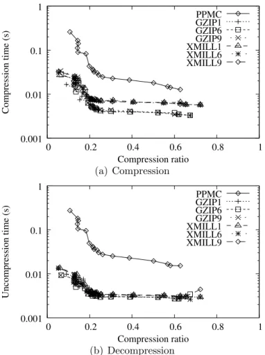
Compression time and compression ratio tradeoff are described in figure 3.15(a). Figure 3.15(b) relates decompression time and compression ratios.
Again gzip had the best compression time performance, although gzip and XMill are almost equivalent when decompressing those files. It is possible to observe the same be-havior described for HTML files relating compression and decompression times with file sizes in these collection, although compressing and decompressing XML files presents a more regular proportion between file size and time than HTML files. As it can be verified in figures 3.16(a) and 3.16(b) for the medical collection and in figures 3.17(a) and 3.17(b) for the Sigmod collection, it is possible to predict, with a certain precision, how long it will take to compress or decompress an XML file on these collection by making a linear regression on those data points. This property is valid for all algorithms analyzed.
XMILL
0.01 0.1 1 10
0 0.2 0.4 0.6 0.8 1
Compression time (s)
Compression ratio PPMC GZIP1 GZIP9 0.001 (a) Compression XMILL 0.01 0.1 1 10
0 0.2 0.4 0.6 0.8 1
Uncompression time (s)
Compression ratio PPMC GZIP1 GZIP9 0.001 (b) Decompression
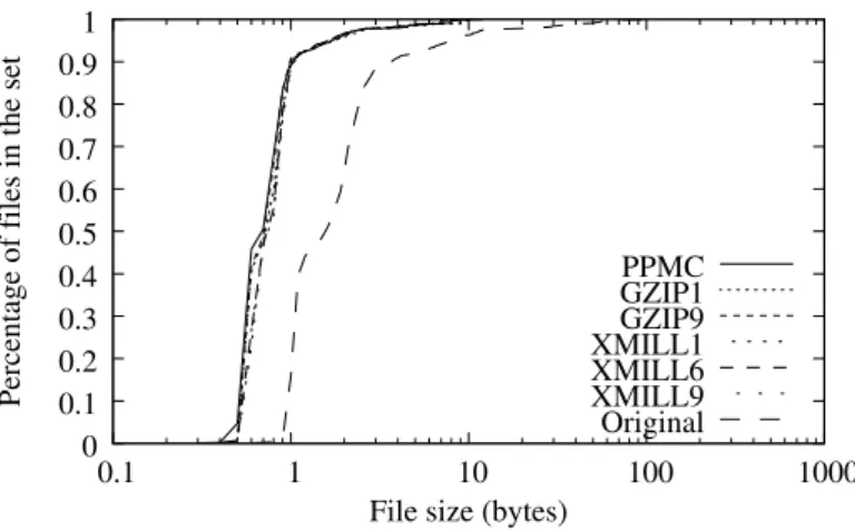
Figure 3.13: Compression and Decompression times versus Compression Ratio (XML Col-lection). Original 0.1 0.2 0.3 0.4 0.5 0.6 0.7 0.8 0.9 1
0.1 1 10 100 1000
Percentage of files in the set
File size (bytes)
PPMC GZIP1 GZIP9 XMILL1 XMILL6 XMILL9 0
Figure 3.14: File size distribution of XML files.
com-XMILL9
0.01 0.1 1
0 0.2 0.4 0.6 0.8 1
Compression time (s)
Compression ratio PPMC GZIP1 GZIP6 GZIP9 XMILL1 XMILL6
0.001
(a) Compression
XMILL9
0.01 0.1 1
0 0.2 0.4 0.6 0.8 1
Uncompression time (s)
Compression ratio PPMC GZIP1 GZIP6 GZIP9 XMILL1 XMILL6
0.001
(b) Decompression
Figure 3.15: Compression and Decompression times versus Compression Ratio (XML Col-lection).
XMILL6
0.2 0.4 0.6 0.8 1 1.2
0 50 100 150 200 250 300 350 400 450
Compression Time (s)
File Size (Kbytes) PPMC
GZIP1 GZIP6 GZIP9
0
(a) Compression time.
XMILL6
0.2 0.4 0.6 0.8 1 1.2 1.4
0 50 100 150 200 250 300 350 400 450
Decompression Time (s)
File Size (Kbytes) PPMC
GZIP1 GZIP6 GZIP9
0
(b) Decompression time.
XMILL9
0.05 0.1 0.15 0.2 0.25 0.3
0 20 40 60 80 100 120
Compression Time (s)
File Size (Kbytes) PPMC
GZIP1 GZIP6 GZIP9 XMILL1 XMILL6
0
(a) Compression time.
XMILL9
0.05 0.1 0.15 0.2 0.25 0.3
0 20 40 60 80 100 120
Decompression Time (s)
File Size (Kbytes) PPMC
GZIP1 GZIP6 GZIP9 XMILL1 XMILL6
0
(b) Decompression time.
Table 3.4: Compressed size of Calgary Corpus files.
ARQ ORIG BZIP2 COMP2 PPMC GZIP9 GZIP6 GZIP1 LZARI LZ77 LZW LZSS COMP1 HUFF
paper5 11954 4837 4763 4507 4995 4995 5424 5321 6507 7017 6069 7559 7633
paper4 13286 5188 5081 4835 5534 5536 6073 5979 7160 7440 6798 7998 8043
obj1 21504 10787 10819 10135 10320 10323 10707 10717 13126 16925 12247 16038 16584
paper6 38105 12292 12455 11683 13213 13232 15282 15520 16865 23301 17609 23837 24230
progc 39611 12544 12896 12018 13261 13275 15455 15333 17007 24464 17531 25922 26111
paper3 46526 15837 16028 15154 18074 18097 20819 20693 22130 23916 23485 27391 27469
progp 49379 10710 11668 10903 11186 11246 13382 12770 15858 23285 15445 30207 30416
paper1 53161 16558 16895 15766 18543 18577 21612 21616 23076 31175 24467 33130 33550
progl 71646 15579 17354 15861 16164 16273 20038 18692 22753 34914 22521 42617 43181
paper2 82199 25041 25453 25871 29667 29753 35078 35098 36653 41664 39703 47540 47830
trans 93695 17899 21023 20668 18862 18985 23966 27979 29710 50543 33641 64340 65434
geo 102400 56921 64590 62673 68414 68493 69810 70385 85922 78753 83183 72405 73084
bib 111261 27467 29840 29915 34900 35063 43871 46222 46094 53844 52591 72792 72941
obj2 246814 76441 85465 80309 81087 81631 93906 90674 106484 302540 103002 187306 194635
news 377109 118600 128047 136068 144400 144840 164199 165143 187823 232808 194435 244496 246606
pic 513216 49759 55461 53022 52381 56442 65540 61301 120385 70215 105311 75066 106949
book2 610856 157443 174085 185883 206158 206687 248846 251451 258339 346529 285942 364788 368521
book1 768771 232598 237380 273629 312281 313376 365005 367576 386475 390807 424147 436926 438577
Table 3.5: Compressed size of Canterbury Corpus files.
ARQ ORIG BZIP2 COMP2 PPMC GZIP9 GZIP6 LZARI GZIP1 LZSS LZW COMP1 HUFF
a.txt 1 37 3 19 27 27 6 27 2 2 3 4
grammar.lsp 3721 1283 1209 1123 1246 1246 1311 1356 1537 2114 2299 2344
xargs.1 4227 1762 1670 1588 1756 1756 1837 1872 2124 2688 2737 2770
fields.c 11150 3039 3106 2942 3136 3143 3360 3674 3841 5313 7159 7224
cp.html 24603 7624 7594 7097 7981 7999 9124 9054 10941 12225 16299 16391
sum 38240 12909 14533 13187 12772 12924 15494 14134 17803 30938 24735 26196
aaa.txt 100000 47 104 130 141 141 2076 481 11808 671 572 12504
alphabet.txt 100000 131 151 224 315 315 2143 660 11834 3402 59307 60160
random.txt 100000 75684 85830 86011 75689 75689 75773 77301 110713 93615 75468 75315
asyoulik.txt 125179 39569 39657 42440 48829 48951 56916 56813 65551 62973 75733 75963
alice29.txt 152089 43202 43964 46220 54191 54435 64625 65144 73117 72318 87358 87864
lcet10.txt 426754 107706 116295 128762 144429 144885 176616 174132 199722 222206 248666 250759
plrabn12.txt 481861 145577 145725 167486 194277 195208 227933 228778 262943 234930 274478 275787
ptt5 513216 49759 55461 53022 52382 56443 61301 65541 105311 70215 75066 106949
pi.txt 1000000 431671 420891 487441 470439 470439 501087 497288 630986 466553 419257 437352
kennedy.xls 1029744 130280 231750 171160 209733 206779 263168 245037 288123 419235 433743 463129
world192.txt 2473400 489583 653089 746881 721413 724606 1121137 917896 1309270 1569210 1545481 1558814
bible.txt 4047392 845623 974496 1050937 1176645 1191071 1450583 1490038 1638297 1851170 2202081 2218604
E.coli 4638690 1251004 1132538 1204968 1299066 1341250 1378814 1526476 1613103 1254888 1176940 1302286
Chapter 4
Adaptive model
The first step to create the adaptive model was to define in which scenarios compression should be used. It is easy to conceive at least two ones: when compression yields a reduction in response time or in power consumption. The second step was selecting the parameters these properties depends on: bandwidth, transmitted file size, compression ratio, type of device where decompression is done, power consumption for transmission and processing, packet error ratio among others. Third, all these parameters were combined together to achieve the previously described goals – reduce time or power costs.
In order to predict when compression can generate some improvement either in re-sponse time or power consumption, the model shown in figure 4.1 is proposed. ModulesT (time) andE (energy) have as inputs the many parameters (as described above) and each one uses its own analytical model to return one value, Vt and Ve respectively, indicating
whether compression is worthy in each case. These values are passed to moduleC, which is responsible for making the final decisionDc. A “weight factor” –WtandWe– is associated
to each module representing its reliability.
Figure 4.1: Predictive model.
the most reliable value). Then,
Wt, We ∈[0,1]
The final decision,Dc, is made through the use of simple mean formula.
Dc =
0 , if Wt =We = 0 Wt·Vt+We·Ve
2.0 , otherwise
A file is transmitted in its original form whenDc <0.5 and it it compressed ifDc ≥0.5.
This means compression will only be made if both decision modules have high reliability values and agree about compression or when one reliability value is higher enough to compensate the other one, in the case of a disagreement.
The next step is feedback. After transmission, data about total transmission time, decompression time if it is the case, the total energy spent by the receiver device, the amount of transferred bits, the amount of bits with errors and the amount of grouped error bits are all collected. All these parameters are used to evaluate the new values of available bandwidth, packet error ratio and reliability factors.
Available bandwidth is calculated based on past transmissions and its formula is
bwi+1 =α·bwi+ (1−α)·
T ami
tti
the last transmission. After running some tests, the value of α was defined as 78 in the experiments.
The packet error ratio is calculated as follows. First, the number of packets between two consecutive error bursts is evaluated with the formula:
P ac= [10
−(T x)· Be
8 ] Tm
where Tx is an exponent representing the error bit rate seen on past transmissions (usual
values are around−5, indicating 1 bit with error in 105 transferred bits),B
eis the amount
of grouped bits with errors (usual values are between 3 and 10), Tm is the packet size
measured in bytes (that´s why it is divided Be by 8) and P ac is the number of packets
between two consecutive error bursts. This last value is used in the formula
Perr =
1 +Di
P ac
where Di is the probability of two consecutive error packets due to the same error burst
and Perr is the packet error ratio.
The new Wt and We values are recalculated based on real and predicted values of
a transmission. If a gain is observed, either in time or energy, the respective factor is increased; otherwise the factor is reduced, as described next.
w←
w+(1−w)
2 , if there is a gain w−w
2 , otherwise
Determining an expected gain is done as follow. Before transmitting a file, each module evaluates two expected values for this operation – one using compression and another one not using it (nc and c indices will refer to not compressed and compressed values respectively). This way, there are two expected transmission times (T Enc and T Ec) and
each module is based on their differences. For instance, if T Ec > T Enc, meaning that
transmission time with no compression is higher than the transmission with compression, then Vt is 1; otherwise Vt is 0. The same idea is applied to energy. After transmitting
the file, whether using compression or not, total time –T T – and total energy –ET – are compared against the expected time/energy values. For instance, if a file is transmitted with compression T T would be compared with T Enc and if an improvement was really
achieved, that is, T T < T Enc, then Wt is increased and it means the module is able
to make good predictions. Otherwise Wt is reduced, meaning the module is doing poor
predictions. After a while, depending on how stable the environment is, the reliability factors will stabilize at some value.
Next it will be presented the description of how the values are evaluated inside each module. First, response time is analyzed. The total expected time to transmit a file is the sum of the expected time spent to send all packets, the expected time spent to resend the ones with errors and the expected time needed to receive all acknowledgments. If compression is used decompression time has to be added. Compression time is negligible since servers have much more power than mobile devices and one compressed file copy could be stored together with the original one, in order to avoid compression at each request. Thus:
T Enc = T sendnc+T resendnc+T acknc
= tamnc
bw +Perr· tamnc
bw + (1 +Perr)·
tamnc
tampkt
· tamack
bw
T Ec = T sendc+T resendc+T ackc+T dec
= tamc
bw +Perr· tamc
bw + (1 +Perr)· tamc
tampkt
· tamack
∆T E = (1 +Perr)·
∆tam bw ·(1 +
tamack
tampkt
)−T dec
wheretamis the file size, tampkt is the packet size,tamack is the acknowledgment size, and
k is a constant that depends on three factors: decompression method used, receiver device and file size.
For energy prediction, only the energy spent by the receiver device for receiving all packets, sending all acknowledgments and decompressing the file should be taken into consideration. Sending packets and compressing files is done by the server but these values can be disregarded as is it supposed that the server is connected to a fixed and infinite power supply.
EEnc = Esendnc+ (Ereceivenc+Eacknc)
= 0 + [Pr·(1 +Perr)·
tamnc
bw +Ps·(1 +Perr)·
tamack
bw ·
tamnc
tampkt
]
EEc = Esendc+ (Ereceivec +Eackc+Edec)
= 0 + [Pr·(1 +Perr)·
tamc
bw +Ps·(1 +Perr)·
tamack
bw · tamc
tampkt
+
Pd·T dec]
∆EE = Pr·(1 +Perr)·
∆tam
bw +Ps·(1 +Perr)·
tamack
bw ·
∆tam tampkt
+Pd·T dec
Ps and Pr are the power values related to sending and receiving packets by the mobile
device. Pd is the processor power spent to decompress a file in the mobile device.
instance, could be measured by constantly sending ping messages or observing the rate at which a TCP buffer is flushed. The packet error ratio could be evaluated in a different way or it could be ignored if it is the case. Energy and time could be evaluated more accurately by changing their formulas or by doing measurements in the hardware itself.
As discussed in Section 3, tests were performed over a collection of text and Web documents in order to determine the constants to be used in the model, as the above formulas assume the use of a predicted compressed file size and a predicted decompression time. To make predictions for these values, Table 4.1 was built. This table gives an approximate compression ratio as a function of compression method and original file size for HTML files.
Table 4.1: Approximate compression ratio as a function of compression method and original size for HTML files.
Kmt
Size (KB) LZSS LZW GZIP PPM 0–1 0.68 0.72 0.60 0.55 1–2 0.58 0.65 0.56 0.46 2–3 0.52 0.60 0.51 0.41 3–4 0.47 0.56 0.46 0.37 4–5 0.45 0.64 0.41 0.35 5–7 0.42 0.50 0.34 0.31 7–10 0.40 0.48 0.32 0.29 10–15 0.36 0.43 0.29 0.25 15–25 0.33 0.38 0.27 0.22
≥25 0.32 0.33 0.25 0.20
Hence, compressed file size is a function, Fc, that can be calculated using the original
file size,T amnc, and the compression constant, Kmt, for the respective M ethod.
T amc =Fc(T amnc, M ethod) =Kmt·T amnc
compression method it suffices to modify theKmt constant to the new proper value.
The time taken to decompress a file is a function,Fd, of three parameters: compressed
file size –T amc, compression method –M ethod, and mobile device to be used –M achine.
Thus:
T dec = Fd(T amc, M achine, M ethod) =K·T amc
= K·Kmt·T amnc
= Kt·Kcl·Kmt·T amnc
whereKcl is a constant related to the mobile device andKtis related to decompression
method and is obtained through linear regression on the results of compression on the HTML (more details on Section 5.2). For instance, Table 4.2 represents Kt values for a
notebook with Pentium processor of 133 MHz and 24 Mbytes of memory. Kt is calculated
through linear regression of all measures taken for decompression time versus file size for the HTML collection (refer to figures 3.9(b) and 3.11) and taking the inclination of the line obtained. For this device, Kcl could be defined as 1. If for instance processor speed
doubles,Kcl could be defined as 0.5 without the need to reevaluate all metrics again.
Table 4.2: Decompression time constant as a function of compression method.
Method Kt
LZSS 4×10⁻⁶
LZW 6×10⁻⁶
PPM 2×10⁻⁴
GZIP 4×10⁻⁶
Chapter 5
Experiments
5.1
Communication protocols
In order to validate the predictive model it is necessary to measure its performance over different conditions. A truly adaptable model should present good performance no matter what the environmental conditions are and should not make performance worse than it would be in a traditional system, that is, with no modifications. In the world of wireless communications,Medium Access Control– MAC – layer plays an important role on defining how and when the wireless carrier is used to transmit data. The protocol used in this layer, in fact, is what distinguish one form of communication from another. For this work, two different types of MAC communication protocols were used: IEEE 802.11 and Bluetooth. A brief description of each one is given next.
5.1.1
IEEE 802.11
In the 802.11 protocol, Basic Service Sets (BSS) are the architectural units. A BSS is defined as a group of communicating devices under control of a unique coordination function (Distributed Coordination Function – DCF), which is responsible for determining when a device can transmit/receive data. Devices can communicate directly (point-to-point) or with the help of a predefined structure. Networks which communicate like the former case are known as ad-hoc networks, and like the later case are known as infra-structured. Infra-structured networks usebase pointsto interconnect devices and to provide mobility across different areas.
There are two basic communicating rates, 1 Mbps and 2 Mbps. Standards 802.11a and 802.11b altered 802.11 physical layers in order to provide higher rates, such as 5.5 Mbps and 11 Mbps (802.11b). The standard 802.11a can achieve 54 Mbps using its own multiplexing technique, which makes communication impossible between 802.11b and 802.11a devices.
5.1.2
Bluetooth
Bluetooth’s main goal is to provide a mechanism to interconnect low-power devices using radio communication. Bluetooth networks allow fast exchange of data and voice among devices such as PDAs, pagers, modems, cell phones and mobile computers.
5.2
Scenarios
For 802.11 experiments, the following scenario was built: an embedded system commu-nicating through a wireless channel with a file server and retrieving files using HTTP protocol. This is similar to a mobile user with a PDA browsing an Intranet of a mall or office. The embedded system used was DIMM-PC/486-I model of Jumptec [30] which is a 486 processor of 66 MHz speed and 16 Mbytes of memory, and Lucent WaveLan 802.11 [31] as wireless card. The receiving, transmitting, and processing costs are specified in Table 5.1.
Table 5.1: Energy costs for 802.11 experiments.
Operation Current (mA) Voltage (V) Power (W)
Transmission 330 5 1.65
Reception 280 5 1.40
Decompression 510 5 2.55 (66 Mhz)
267 5 1.33 (33 Mhz)
In order to apply the model, all values for the parameters had to be evaluated again for this system, as described in Chapter 4. As the only changes happened in the hardware (and not in the compression algorithms), ratio compression values remained constant. Figure 5.1 shows the linear variation of decompression time versus file size for the HTML collection for files smaller than 15 Kbytes. The new Kt value, which can be obtained by linear regression, was defined as 1,875×10−5 and K
cl was set to 1 on this new system.
0 0.05 0.1 0.15 0.2 0.25 0.3
14KB 12KB 10KB 8KB 6KB 4KB 2KB
Time (s)
Compressed File Size
Figure 5.1: File size versus decompression time for files smaller than 15 Kbytes.
parameter had to be reevaluated for these machine.
The actual implementation of this model required the insertion of new fields on the HTTP header [35], containing information about the last transfer (figure 5.2). These pieces of information are piggybacked to the server when a new request is sent. Before answering the request, the server will pass through the feedback step of the adaptive model with new data. Many servers already retain information about client interaction through the use of sessions, hence inserting new data to these structures is trivial.
Figure 5.2: Scenario of 802.11 experiments.
to store the information related to the last transfer until the next request. This can be accomplished by maintaining a set of few variables in the memory while the application is active. Another option for implementation is putting all intelligence on the clients. This requires some modifications in the model, since the client cannot guess the requested file size. A possible solution is to let a client evaluate the range of file sizes that could be compressed and send this information to the server. This range would be analyzed by the server and the requested file would be sent with or without compression depending on it. This would imply more memory/energy costs in the clients with the model’s calculations but it frees the server of the burden to store information about each client.
5.3
Results
For the 802.11 experiments, 190 Web files were randomly selected from the HTTP collection for testing. Figures 5.3(a) and 5.3(b) plots response time versus file size for bandwidth of 1 Mbps for each of the three models: no compression at all, always compressing the file and the adaptive model. Figure 5.3(a) compares the three models for files with size smaller than 10kbytes and figure 5.3(a) does the same for size larger than 10 kbytes. It is possible to observe that the adaptive model fits into the best case in both situations, that is, for files smaller than 10 kbytes adaptive model decides that files should not be compressed; for the other files, the best case occurs when files are compressed before transmission. Around 10 kbytes both times (transmission with and without compression) are approximately the same. According to [36], most of the replies are less than 3 Kbytes for online wireless clients – the ones which demand HTTP pages one by one when they browsing on the Internet – and less than 6 Kbytes for offline clients – the ones which demands all pages before browsing through them. Thus, compressing all responses would not be a good policy, even for a low bandwidth link.
0 0.02 0.04 0.06 0.08 0.1 0.12
1 2 3 4 5 6 7 8 9 10
Response Time (s)
File Size (Kbytes)
Adaptive Compressed Not compressed
(a) File size smaller than 10 Kbytes.
0 0.1 0.2 0.3 0.4 0.5 0.6 0.7 0.8
10 20 30 40 50 60 70
Response Time (s)
File Size (Kbytes)
Adaptive Compressed Not compressed
(b) File size larger than 10 Kbytes.
Figure 5.3: Response time for adaptive, compressed and not compressed models.
not compressed models for all tested files. For the small files, gains are about 60 to 70% for sizes ranging from 1 to 2 Kbytes, decreasing out of these limits. For large files, there is a continuous increasingly gain as the size gets bigger. For a size of approximately 50 Kbytes, gains are about 20 to 30%.
−0.6 −0.4 −0.2 0 0.2 0.4 0.6 0.8
10 20 30 40 50 60 70
Percetual gain (%)
File Size (Kbytes)
Adaptive over Compressed Adaptive over Not Compressed
Figure 5.4: Percentual gain of adaptive model over compressed and not compressed models.
0 10 20 30 40 50 60
0 20 40 60 80 100 120 140 160 180 200
Energy (J)
Files in request order
Adaptive Compressed Not compressed
Figure 5.5: Accumulated consumed energy of adaptive, compressed and not compressed models
would not have the behavior as seen before.
Next figures show how compression depends on the device as much as in the file size and on bandwidth. In Figure 5.6, bandwidth was modified to 2 Mbps and all gains due to compression disappeared, since then decompressing the file taken much longer than the time saved in its transmission. The adaptive model was able to adapt to the best case.
0 0.05 0.1 0.15 0.2 0.25 0.3 0.35 0.4 0.45 0.5
10 20 30 40 50 60 70
Response Time (s)
File Size (Kbytes)
Adaptive Compressed Not Compressed
Figure 5.6: Response time for adaptive, compression and not compression models using bandwidth of 2 Mbps and processor speed of 66 MHz.
Next (figure 5.7), processor speed was changed to 33 MHz and the same experiments were executed as before using 1 Mbps as bandwidth. As the same device was used – the only difference was clock speed – it was enough to modifyKcl to 2 and to use the respective
energy consumption values (Table 5.1). Again, time saved with compressed transmission is not compensated by the time taken to decompress a file in such a slow system.
The conclusion is that even for the same bandwidth channel and for the same device compression decision should be done individually and a static solution would fail to give the best performance always.
0 0.1 0.2 0.3 0.4 0.5 0.6 0.7 0.8 0.9
10 20 30 40 50 60 70
Response Time (s)
File Size (Kbytes)
Adaptive Compressed Not Compressed
Figure 5.7: Response time for adaptive, compression and not compression models using bandwidth of 1 Mbps and processor speed of 33 MHz.
which compression could be used. The graph in Figure 5.8 shows the large difference in response time for adaptive and not compression models.
0 0.5 1 1.5 2 2.5 3 3.5
10 20 30 40 50 60 70
Response Time (s)
File Size (Kbytes)
Adaptive Not compressed
Figure 5.8: Response time for the Bluetooth protocol.
5.3.1
An analytical view
It is possible to plot response time as a function of file size, bandwidth, and processor speed using the time formulas of the analytical model (Chapter 4). By making some assumptions like null packet error rate, graphs like the ones shown in Figures 5.9(a) and 5.9(b) can be obtained. These graphs offer an analytical view of the model, which is summarized in Figure 5.10.
Compression Not compression
50 40
30 20 10
File Size (Kbytes) 1Mb
1.5Mb Bandwidth (Mbs)
0.2 0.4 0.6 0.8 1 Response Time
(a) Bandwidth 1 Mbps; Processor speed 66 MHz.
Compression Not compression
50 40
30 20
10
File Size (Kbytes) 1Mb
1.5Mb Bandwidth (Mbs)
0.2 0.4 0.6 0.8 1 Response Time
(b) Bandwidth 1 Mbps; Processor speed 33 MHz.
Figure 5.9: Response time as a function of file size and bandwidth.