..
... ~FUNDAÇÃO
... OETUUO VARGAS EPGE
Escola de Pós-Graduação em Economia
SE\110:/\RIOS
DE PESQUISA
ECO:-;ÓMICA
"Growth, Dlstrlbution and School Policy"
Prof. Eduardo C. Andrade (IBMEC/SP)
l.()CAII
Fundação Getulio Vargas
Praia de Botafogo, 190 - 100 andar - Auditório
UATA
01107//99 (58 feira)
•
Growth. Distribution and School Policy
Eduardo C. Andrade
U niversity of Chicago
E-mail: [email protected]
February 1997
Abstract
This paper investigates the relationship between growth, income inequality, and educational policies. An endogenous growth model is built in which there are two types of labor, skilled and unskilled, and the quality of the labor force (measured by the fraction of skilled workers) will ultimately determine the eco-nomic growth rate. We show that multi pIe inequality and growth paths may arise. Countries will not necessarily converge to the same economic growth and income distribution. When the proportion of skilled workers is low, the economy grows slow, and the Gini coeflicient is high. Low expected growth rate inhibits invest-ments in human capital and the quality of the labor force tomorrow turns out to be low again, keeping the economy in the bad equilibrium.
We then analyze the effects on growth and inequality of two types of govern-ment intervention: introduction of public schools and vouchers. Both types can induce the economic agents to invest more in education. The consequence will be an increase in the quality of the labor force, leading to higher growth rates and less inequality.
•
..
1 Introduction
It is a welI-established idea that there is a close link between investments in human capital and economic growth. Empirical evidence shows that mea-sures of educational attainment are important variables to explain future growth rates.l In other words, the quality of the labor force is a crucial indi-cator of a country's prospects of future development. Moreover, the greater the quality of the labor force, the lower is the proportion of unskilIed work-ers, and "greater the scarcity value of unskilled labor." Hence, the income disparity between the bottom and the upper classes is lower leading to less income inequality.2 According to this reasoning, countries with different
la-bor force quality should grow at different rates and register different income distribution. Clarke (1995) finds that different measures of inequality are negatively and significantly correlated with the growth of per capita GDP using data for 79 countries. However, should one expect alI countries to con-verge to the same economic growth as welI as to the same income inequality? This is the first question addressed in this paper.
The empirical evidence suggests that it might not be the case. The c1assical example is the comparative performance between Latin American and East Asian countries. The latter has grown faster with a more equitable income distribution since the 50's. Moreover, Africa ranks much the same in terms of inequality as Latin America with very poor economic performance. Furthermore, numerous cross-chapter growth regressions indicate that initial inequality is detrimental to long-run growth.3 About these results, Bénabou
(1996) writes: "a one standard deviation decrease in inequality raises the annual growth rate of GDP per capita by 0.5 to 0.8 percentage points ( ... ) imply(ing) an income gap of about 25% after 30 years."
If the quality of the labor force is so important as it affects growth and income distribution, policymakers should design policies to encourage invest-ments in education to increase the fraction of skilIed workers in the society. These policies might be desirable even if there are no perfect capital markets to finance education. However, in particular, if there is no capital market to finance investment in human capital and there are decreasing returns in these investments, the government ought to equalize the access to
educa-lSee, for example, Levine and Renelt (1992).
2The World Development Report (1992) suggests that it is the distribution of human capital and not of physical assets that is very closely related to the distribution of income. Stokey (1996) writes: "while inherited wealth may be a significant contributor to persis-tence in the upper tail of the income distribution, for the rest its importance is modest and for the bottom half it is apparently of little or no consequence. It is persistence in earnings that has the greater infiuence, because earnings are the bulk of national income and because earnings are important in ali ranges of the income distribution."
tion. This seems to have been the motivation of policymakers in East Asian countries when they chose to emphasize primary and secondary education in detriment to tertiary education back in the 50's. As another example, Chile is currently implementing a major educational reformo The numbers of hours that a public school student wiIl stay in school per day will dou-ble, reaching 8 hours, the same as current hours in private schools. Two questions come to mind. Can a school policy effectively increase the quality of the labor force, leading to higher growth rates and less inequality? Are investments in public schools and the supply of vouchers to be spent in pri-vate schools alternative ways to reach this objective? This paper addresses these two questions.
FinaIly, we examine if these government interventions are desirable. Mem-bers of the current generation will pay the price and the benefits will come only in the future through higher growth rates and income. If individuals are very impatient, the net benefit may be negative.
To investigate the relation between growth, income inequality, and edu-cational policies and to address the above questions, an endogenous growth model is built. A simplified version of the theoretical framework in Stokey (1988) and Young (1991) is used in which the accumulation of knowledge, through economywide learning by doing, is the only 'engine' of growth. The idea is that a firm that increases its production learns simultaneously how to improve the quality of the good produced. Growth is measured by the rate of increase of this quality leveI. To retain the framework of perfect competi-tion, it is assumed that alI improvements in the quality of the good produced are unintended by-products of the production process and that they imme-diately become common knowledge. On the other hand, one could interpret that "the learning and spillovers involve human capital and that each pro-ducer benefits from the average leveI of human capital in the economy ( ... ). Thus, instead of thinking about the accumulated knowledge or experience of other producers, we have to think here about the benefit from interacting (freely) with the average person, who possess the average leveI of skills and knowledge." (See Barro and Sala-i-Martin, 1995) Under this interpretation, the economy would grow faster the greater is the quality of the labor force. Furthermore, it is used a sim pIe overlapping generation model with in-tergenerational altruism as in Loury (1981). There are two types of agents, skilled (with high leveI of human capital) and unskiIled (with low leveI of human capital). The offspring's earning capacity, and therefore his economic status, depends primarily on his parent's investment in his human capital. The greater this investment, the more likely a child will become an indi-vidual with high leveI of human capitaL The quality of the labor force is measured by the fraction of skilled workers.4
i
•
These two types of agents are the only inputs in the production function. As an individual with high leveI of human capital is more productive than one with low leveI of human capital, the greater the quality of the labor force the more experience is accumulated in the production processo Hence, faster the economy grows. Moreover, the greater is the proportion of skilled workers greater is the scarcity value of unskilled labor and less unequal is the income distribution.
The focus is on stationary equilibrium that arises from this setup, where the growth rate (measure by the increase in the quality ofthe good produced) and the fraction of skilled workers are constant. It is shown that multiple growth and inequality paths may arise. The path with higher growth rate is also the one with more egalitarian income distribution, where the latter is measured by the Gini coefficient. The explanation runs as follows. We as-sume, as in Azariadis and Drazen (1990), a "technological externality with a 'threshold' property" that permits returns to scale to rise very rapidly whenever the quality of the labor force reaches a certain point. In such a framework, an economy with a low quality labor force today is expected to grow slowly. Agents with forward-Iooking behavior realize it and they are discouraged to invest in their child's human capital as the benefits of these investments are perceived to be low in such stagnant environrnent, despite the great differences in income of skilled and unskilled workers. In a more technical way, the slower the expected economic growth rate, the greater is the discount imposed by the present generation on future consumption in the intertemporal utility functions that guide consumption and investment in human capital decisions. Hence, low expected growth rate inhibits invest-ments in human capital and the quality of the labor tomorrow turns out to be low again, maintaining the economy in an equilibrium with very unequal income distribution and low growth rates.
,
Finally, we examine the welfare consequences of these interventions and conclude that they may be Pareto improving. In other words, the utility leveI of both type of agents may be greater after the government intervenes either through public schools or vouchers.
Azariadis and Drazen (1990) and Becker, et aI. (1993) are examples of endogenous growth models with multiple balanced growth path. However, they do not consider redistribution issues as they work with a representative agent framework.
The closest paper related to this one is Glomm and Ravikumar (1992). They develop an endogenous growth model with intergeneration altruism that tries to connect private and public education, income inequality, and economic growth. There are important differences between this paper and theirs: (i) the current generation values the wealth they pass on to their descendants in their model whereas the current generation values the next generation's utility in my model, (ii) they do not allow a mixed regime with private and public education, (iii) they do not consider a voucher system, and (iv) they do not analyze welfare effects from different educational regimes.
To my knowledge, Chou and Talmain (1996) is the only paper that ad-dress the welfare consequences of a redistribution policy. They build an endogenous growth model in which the wealth of the households determines their permanent income, which in turn determines their labor supply, and ul-timately the growth rate. They show that it is possible for the rich to be bet-ter off as a result of a wealth distribution. They experience a loss of wealth today but benefits from increase growth and income in the future.However, the accumulation of human capital is not the 'engine' of growth and, con-sequently, they do not consider the welfare effects of different educational policies as it is done here.
2
The Empirical Evidence
Several empirical studies have analyzed the link between income distribu-tion and economic growth. They run cross-country growth regressions in which the dependent variable is either the average growth of the per capita income or the average growth rate of GDP over a long period of time. They include, among other explanatory variables5, a measure of income
distri-bution. These studies differ one from another mainly because either they use different measures of income distribution or they consider different time periods.
These empirical investigation use a measure of the income distribution variable at the start of the period over which growth is measured. This procedure is employed in order to circumvent potential endogeneity and reverse causation problems.
To my knowledge, Persson and Tabellini (1990) and Alesina and Rodrik (1991) are the first papers that run growth regressions using a measure of income distribution as an explanatory variable. They initially develop a theoretical model to argue that greater inequality slows growth. The the(}-retical argument in both papers is similar. High leveIs of income inequality generates greater conflict over distributional issues and encourages govern-ment to impose higher taxes to reduce it. The implications of these higher taxes are a reduction on the rate of return on private investments, limiting capital accumulation and reducing the economic growth rate.
Persson and Tabellini (1990) use the average growth rate of per capita real GDP over the period 1960-1985 as the dependent variable. They use the fraction of income received by the third quintile of the distribution (this variable is called 'middle') and the Gini coeflicient for the distribution of land ownership as measures of income distribution6. Their results led to the
conclusion that "a more unequal size distribution of income is bad for growth in democracies."7 Moreover, they conclude that the effects of distribution on growth are also quantitavely important: "a one-standard deviation change
5 Among these explanatory variables, two are always incorporated in these regressions: the initial leveI of per capita income and a variable that indicates the educational at-tainrnents of the population. As presented below, Clarke (1995) shows strong empirical support to the link between income distribution and economic growth for different spec-ifications of the growth regression.
6They obtain similar results when they replace 'middle' by the percentage of income received by the top 5% of the population or the Gini coefficient obtained from the distri-bution of pre-tax income.
•
in (the measures of income distribution) both affect average annual growth byat least half a percentage point."
Alesina and Rodrik (1991) use the average growth rate during 1960-85 as the dependent variable. They run regressions with six different distributional indicators. These indicators are the income shares of each ofthe five quintiles in the population and the income share of the top five percentile. The idea is that "increases in the income shares of the poorer quintiles are associated with increases in growth, while increases in the income shares of the richest quintile and of the top five percent are associated with decreases in growth." All coeflicients related to the distributional variables in the regressions have the expected sign but only the third and highest quintiles and the top five percentile are statistically significant.
The next experiment executed by the authors was to divide the sample in two groups, democratic and non-democratic countries, and to run separate regressions for each one. All coeflicients associated with the distributional variables in the latter group have the expected sign but they are not statisti-cally significant. In contrast, the results obtained with the former group are similar to the ones when the fuII sample is included. About these results, they write: "These results suggest that growth may be particularly sensitive in a democracy to the income shares of the middle class and of the richest quintile. The income share of the poorest individuaIs may exert little infiu-ence. One possible reason is that the middle class is likely to be politically much more active than poorer income groups."
Clarke (1995) is the most complete empirical investigation of the link between growth and income distribution. The dependent variable is the av-erage growth of per capita GDP over the period 1070-1988. He also uses better measures of income distribution. These measures are: the coeflicient of variation, the Theil's index, the Gini coeflicient and the ratio of the share of total income earned by the poorest 40 percent of the population to the share of income earned by the richest 20 percent of the population. The author has three objectives in the paper: to show that an initial unequal income distribution is detrimental to growth, to show that this link is im-portant in democratic countries as well as non-democratic ones, and, finally, to show that these results are robust across different specifications for the growth regression.
The coeflicients of the distributional variables have the expected sign, that is, a greater initial inequality leads to lower growth, and are statistically significant. According to the author's estimation, a reduction in inequality from one standard deviation above to one standard deviation below the mean can increase the long-term growth rate by up to approximately 2.5%.
..
inequality is detrimental to growth only in democratic countries, as indicated in other studies mentioned above. He concludes that inequality appears to have a negative impact on both types of regime, with the interaction term being statistically insignificant in many regression and the distributional variable being statistically significant.
Finally, Clarke addresses the issue that the sign and significance of vari-ables in cross country growth regressions are highly sensitive to the inclusion or exclusion of variables that are considered significant in other studies. He follows the procedure proposed in Levine and Renelt (1992) to test the ro-bustness of regression results. Departing from a 'Barro type regression' as the base regression, he introduces variables chosen as proxy for aspects of monetary policy, trade policy, and macroeconomic and social stability. The significance of the distributional variables is robust across different specifi-cations of the growth regression.
Bénabou (1996) conducts a survey of other papers which considers the link between income distribution and economic growth. The main conclusion he draws from this survey is the following: "These regressions, run over a variety of data sets and periods with many different measures of income distribution, deliver a consistent messge: initial inequality is detrimental to long-run growth."
Bénabou performs an additional empirical investigation. He checks if countries are converging to the same leveI of inequality. In order to test it, he basically run regressions with the rate of change in the Gini coeffi-cient on a constant and the initial value of the Gini. His conclusion is the following: "The general picture which emerges at the end of this empiri-cal exercise is thus a mixed one: general stability in the world distribution of Ginis, within which countries and regions seem to be experiencing some non-negligible amount of relative mobility. The question of whether there is actual convergence or whether countries oscillate around distinct long-run levels of inequality still awaits a definit answer." He emphasizes that the limitations of the data are the main obstacle to a more definite answer.
3
The Envi ronment
constant over time. Each generation consists of a continuum of agents with measure one.
It is assumed that only one good is produced in the economy, good Y, but it can potentially be supplied in different quality leveIs, indexed by z.8
At time t = O, it is assumed that producers have the knowledge to produce good Y with quality Zo. In order to simplify the problem, it is also assumed that it is produced and consumed only the good with the highest quality leveI available at each point in time. 9 The improvement in the quality leveI
of good Y will depend on the experience accumulated in producing a good with lower quality leveI. Let Y (z) be the total output produced today of good Y with quality leveI z. Therefore, the newest and highest quality leveI available next period,
z',
will be given by:z' =
[1
+
g(Y(z))]z (1)where:
Assumption 1: 9 is a function with the following properties: (i) g(O) =
O; (ii) 9 is continuous; and (ii) g'(.)
2:
O . •The spillover of the experience in producing a less sophisticated good to the production of a more sophisticated one is the only 'engine of growth' in this modeI. This formulation captures the same idea to explain growth as the models developed by Stokey (1988) and Young (1991). The difference is that in those mo deIs the knowledge to produce an immediatly more sophisticated good is acquired only after the country has accumulated enough experience in producing an immediatly less sophisticated good and the productivity in the production of the good of any quality leveI decreases over time. Here we use a simplified version in which the greater the production of the single good with a certain quality leveI today higher will be the jump in the quality leveI of this good tomOITOw.
Two types oflabor - high leveI ofhuman capital labor Nh , and low leveI
of human capital labor N1 - are used to produce the single quality leveI of good Y available at each point in time. The single technology, which has constant returns to scale, produces goods that can be consumed, or invested in education. There is no physical capital in this mode!. As in Stokey (1996), "labor provides two distinct productive services, which we may think of as physical effort ("brawn") and mental effort ("brains")". We assume that
8 Alternatively, y could be seen as a bundle composed of many different goods consumed always at fixed proportions at ali possible quality leveIs where the quality of all goods are increased at the same time.
•
workers with high leveI of human capital can provi de both services, while workers with low leveI of human capital supplies only the former - that is, in order to be able to execute more sophisticated tasks the individual must acquire a higher leveI of human capital. The aggregate prod uction function is the following:
Y = ANt:(Nh
+
NZ)l-Qwhere A is a positive constant and O
<
a<
1.10On a per capital basis, the technology is:
(2)
(3)
where y is the output per capita and q is defined as the the fraction of the population with high leveI of human capital, i.e., q
=
N:.tNz.H
Using equation (3) in (1), we get:
z'
=
[1
+
g(AqQ)Jz =} z'=
'ljJ(q)z(4)
where:
'ljJ(q) =
[1
+
g(AqQ)J.From the above equation, one can conclude that the higher the fraction of individuaIs with high leveI of human capital (q), greater the total production today and, hence, greater the quality of the good tomorrow. Economic growth in this model is measured by 'ljJ(q) , the rate of good Y's quality increase. Therefore, q and economic growth are positively correlated. In
other words, q can be seen as a measure of the quality of the labor force. An economy would grow faster, the greater it is the quality of its labor force. Equation (4) indicates the highest quality leveI of good y available next period.
All parents have identical preferences. These preferences manifest inter-generational altruism. Each parent takes as given his leveI of human capital, high (h) or low (l), earns a wage w and decide how much to invest in his offspring's education and spend on consumption. If a parent invests E units of good Y in his offspring's education, with probability 7r(E) and 1-7r(E),
respectively, his child will acquire h, a high leveI of human capital, and l, a low leveI of human capital. Therefore, there are two types of individuaIs at each date.
10 As only the highest quality leveI of good Y will be produced at each point in time the index z wiil be omitted from now on.
Assumption 2: 7r is a function with the following properties: (i) 7r is continuous; (ii) 7r(0) = O; (iii) 7rE
>
O; (iv) 7rEE<
O; and (v) O ::; 7r<
1. •The assumption that the function 7r is increasing implies that a child is more likely to become an individual with high leveI of human capital the greater is his parent's investment in his education. However, a parent can never be sure that his offspring will turn out to be a high type individuaIs
as
7r is lower than 1. We also assume that the function 7r is concave. This assumption is made in order to capture the notion that there are decreasing returns on educational investments. There is empirical evidence to support it. Galor and Zeira (1993) cites empirical studies that estimate that yearly social returns to investment in education in developing countries are: 26% for primary education, 17% for secondary education and 13% for higher education. Stokey (1996) cites empirical evidence of the rates of return on investments in child's human capital for the United States: 17-22% for lower education, 15-16% for high school, 12-13% for college, and 7% for graduate school.The individual type x's actions (x E {h, l}) can be summarized by the outcome of the following dynamic programming problem:
(as
only one qual-ity of the good Y will be produced at any point in time, we set the price of this quality leveI produced at each time to be one)V(z, q, x) = max
u(C
x , z)+,B{
7r(Ex)V(z', q',h)+
[l-7r(Ex)]V(z', q', ln (5) ex ,Exsuch that:
where:
(i) V(z,q,x) is the parent type x's utility;
(ii) V(z', q', x) is the child's utility if he turns out to be type x; (iii) Cx is the total consumption of individual type x;
(iv) W x is the wage paid to an individual with human capital x;
(v) Ex is the total expenditures on offspring's human capital of parent type x;
(vi)
,B
is the degree of altruism and O<
,B
<
1;(vii)
u(C
x ,z)
is the current utility of individual typex
if consumesC
xunits of the good y with quality z;
(viii)
u
c (.,.)>
O,u
cc (.,')<
O, andu
z (.,.)>
O.Implicit in the above set-up is the assumption that there is no market to finance investments in education.12 The same assumption is made in Loury
(1981) among others.
In addition to his type (h or l), each individual also takes as given z and
q. These are the two state variables in the model. When the consumer goes to the market to buy good Y he will get higher utility as greater z is but he can not affect the quality of the product available. As mentioned above, higher q implies greater economic growth (and greater utility growth) but each individual can not affect q.
The above formulation implies that each parent can not affect the pos-sible values of his offspring's utility, V
(z',
q', l) and V(z',
q', h). In other words, he can not affect the environment where his children willlive tomor-row. However, he can infiuence the type his children will turn out to be through his investment in his child's education, i.e., if his child will have utility V(z', q', l) or V(z',q', h).•
(
0)1-0-Assumption 3: u( C, z) =
\-a .•
In the appendix, where alI results are derived or proved, we show:
Proposition 1: Under assumption 3, V(z,q,x) = Zl-a v (q, x), where:
In the above propostion, we reformulated the individual's problem and showed that in deciding which optimal decision to take with respect to con-sumption and investment he does not take into account the leveI of z. He considers only the growth rate of z, that is, the economic growth rate. There-fore, q becomes the only state variable relevant in this model as it determines the economic growth rate.
Let Ix(q) and cx(q) be the optimal policy functions for the problem (6) of the representative individual type x.
Assumption 4: j3'ljJ(l)l-a
<
1. •Proposition 2: Under assumptions
1-4,
there exists a unique value func-tion v (that is bounded and continuous) satisfying (6). For each q, the max-imum in (6) is attained by a uni que value Ix(q), and the policy function I is continuous . •4 Competitive Equilibrium
"
Firms act as price-takerso They, taking as given prices and wage rates, decide how much units of labor of the different skills to hire in order to produce good Yo 13Note that, as in Stokey (1991), "since learning spills over completely
(000)
to other fums, it is not in the interest of any producer to suffer current losses in order to accelerate learningo"A representative fum maximizes profits which are given by:
(7)
As there is perfect competition in all markets, labor is paid its marginal producto Therefore, the fust-order conditions for the representative fum's problem are: (using the fact that Nh
=
q and N1=
(1 - q))(8)
and
(9)
Note that fums earn no profitso
It is obvious that parents would invest in their child's human capital only if their child can benefit by this investmento The benefit in this model is obtained through a higher leveI of human capital that will lead to higher wageso The wage difference between an individual with high leveI of human capital and the one with low leveI of human capital is the premium for investing in educationo Hence, this premium must be positive in order to have positive investment in education in equilibriumo Looking at equation (9), one can see that this premium is positive for any possible value for q (recall that O ::; q ::; 1) and it is decreasing in q (ioeo, d(W~-WI)
<
0)0
The income share of the individuaIs with low leveI of human capital is given by: (using equations (3) and (8))
Wl(l
y
-
q) = (1 - a)(1 _ q)oWe can compare the Gini coeflicient for two economies with different q'so Let qA and qB denote, respectively, the fraction of individuals with low leveI of human capital in economies A and B such that qA
<
qB o Point A in figureI indicates that the fraction (1 - qA) of the population in economy A, the bottom income class, holds the fraction (I-a) (l-qA) of the total incomeo Point B is the correspondent plot for economy B o Looking at figure 1, one can see that the Gini coeflicient in economies A and B are given, respectively, by the area of the triangles O AC and O BC o The fact that 1:10 AC>
1:10 BC13 As it is assumed that only the highest quality of good Y will be produced at each
indicates that economy A has a greater Gini coefficient than economy B, i.e., it has a more unequal income distribution. As discussed above, economy A
would also grow at a lower rate in comparison with economy B as qA
<
qB.Therefore, if there are two economies with different q's, the one with higher
q will grow faster and have a more egalitarian income distribution. The only exception to this rule will occur in the extreme case when q = O. In that case, all individuals will have the low leveI of human capital, and economic growth rate will be zero. However, this is not an interesting case as it would imply a Gini coefficient equal to zero which is not observed empirically.14
10. Appendix 2
FIGURE 1
Fraction ~,
01'
'1'
I
Income(l-~) (l-qJ
(l-~ (l~)
I
i-.,,----i
I
i
i
I· . . . . . . .
~
.
. .
.
.
I I
I
I
I
o .. "
. -_._ ... ~_._.~." ... " ....".
1-~
68
c
1-<lA
Fraction
of
Let's now turn to the household's dynarnic problem. Each individual, forming expectations about v(q',h) and v(q',l) (or q') and taking as given wages and prices, make decisions about investment in offspring's education and total consumption. It is assumed that they have rational expectations. The first-order condition for the dynamic problem of the representative household type x is given by:
This equation indicates that each individual equates the marginal benefit of consuming one additional unit of the good Y to the marginal benefit of investing one additional unit ofthe same good Y in his child's human capital.
The law of motion for the state variable q is:
q' = 1f(h(q))q
+
1f(Iz(q))(l - q). (11)Note that while there is individual uncertainty about the leveI of his child's human capital, there is no aggregate uncertainty. If a fraction q of the population decides to invest E* in his child's education, we know that 1f(E*) of those will succeed in giving a high leveI of human capital to their offspring.
Definition 1: A recursive competitive equilibrium, given the initial
con-dition qo, qo E (0,1], is defined to be value functions v : [0,1] x {x} -+ R,
x = h, l, policy functions Cx : [0,1] -+ R+, and Ix : [0,1] -+ R+, an economy-wide law of motion for the fraction of individuals with high level of human capital
Q :
[O,
1] -+[O,
1], and factor prices functions Wx :[O,
1] -+ R+ suchthat:
(i) v satisfies the household problem (6);
(ii) Cx and Ix are the optimal policy functions for (6);
(iii) the wage functions are given by equations (8) and (9);
(iv) the economy-wide law of motion for q is given by equation (11).
This competitive equilibrium implies an economy-wide law of motion Z: [0,1] X R+ -+ R+ for the quality of good Y. This law of motion is given
by equation (4).
5 Stationary Equilibrium
5.1
Theoretical ExaminationDefinition 2: A stationary growth path is a competitive equilibrium in which the fraction of individuals with high level of human capital, q, is con-stant.
This condition pins down the invariance (with time) or growth rate of the remaining variables on a stationary growth path. It follows from (4) that the quality of good Y, the measure of economic growth, will grow at the constant rate 'ljJ(q). From (8) and (9), we get the implication that, respectively, w[
and Wh are time-invariant. Hence, total expenditures in human capital, Ex,
and consumption,
ex,
are also constant, as can be seen from (10). From equation (3), it follows that the number of units produced of good Y is time-invariant too.With the constancy of q, wx, and Ex, we can use the result in proposition
1 to infer how V and v evolve over time in this stationary equilibrium. Using equation (4), we get:
V(z',q',x) V(z',q,x)
(Z')I-UV
(q', x)-
-V(z, q, x) V(z, q, x) (z)1-u v (q, x)
Therefore, the household's utility V grows at a constant rate given by
'ljJ(q)l-u and Vx is a constant, where Vx
=
v(q, x). The growth in the utilityV refiects the increase in the quality of the good available to the household.
The quality of consumption, investment in education, and wages is increasing over time in this stationary equilibrium, only the quantity is constant. In that sense we can say that both types of agents are becoming wealthier over time.
There are seven equations that characterize this stationary equilibrium with seven unknowns (Ez, Eh' q, Wh, W[, Vz, Vh):
-the two first-order condition for the firms' problem:
(12)
and
+A a-I
Wh = W[ aq . (13)
-the first-order condition for each type of agent:
(14)
(15)
-one equation for each v:
and
-the law of motion for q (imposing the condition q = q'):
(18)
We now turn to the task of proving that there is at least one solution to this system of equations. We start by choosing a functional form for the probability function 1r.
Assumption 5: 7r(E) = k
(~)1-0,
where 0< k,e
< 1. •This above functional form for 7r satisfies the properties in assumption 2. In particular, the parameter A enters in this functional form to guarantee that 7r(.)
<
1, for any possible E. The maximum units of good Y that can be produced at any point in time is equal to A. This is the total output when q=
1. We have that 7r(A)<
1, as k<
1. Hence, there will always be two types of agents in the economy and no parent can assure through investment that his child will turn out to be the high type individual.In the following proposition, we prove existence of stationary growth path to a particular case in which (j = () in order to get an analytical solution.
This assumption implies that both types of agents spend the same fraction of their income investing in their child's education. To work out this particular case is interesting because it is possible to understand which assumption drives the result of multiple balanced growth path, discussed below.15
Proposition 3: With assumptions 1, and 3-5, if (j = (), then there
exists at least one stationary growth path . •
In order to capture the phenomenon of multi pIe balanced growth, we borrow the idea of "technological externality with a 'threshold' property" used in Azariadis and Drazen (1990). This technological feature "permits returns to scale to rise very rapidly whenever economic state variables, such as the quality of the labor, take on values in a relatively narrow 'criticaI mass' range." 16 We then assume that the learning by doing technology exhibits
increasing returns when the fraction of skilled workers in the society passes a certain leveI, say, qL. These returns are decreasing when q goes beyond a certain leveI, say, qH.
Assumption 6: The function 9 has the following properties: (i) g' ~ O
for any q such that O
<
q<
qL, (ii) g'>
O and g">
O for any q such thatqL
<
q<
qH, and (iii) g'>
O and g"<
O for any q such that qH<
q<
1; where O<
qL<
qH<
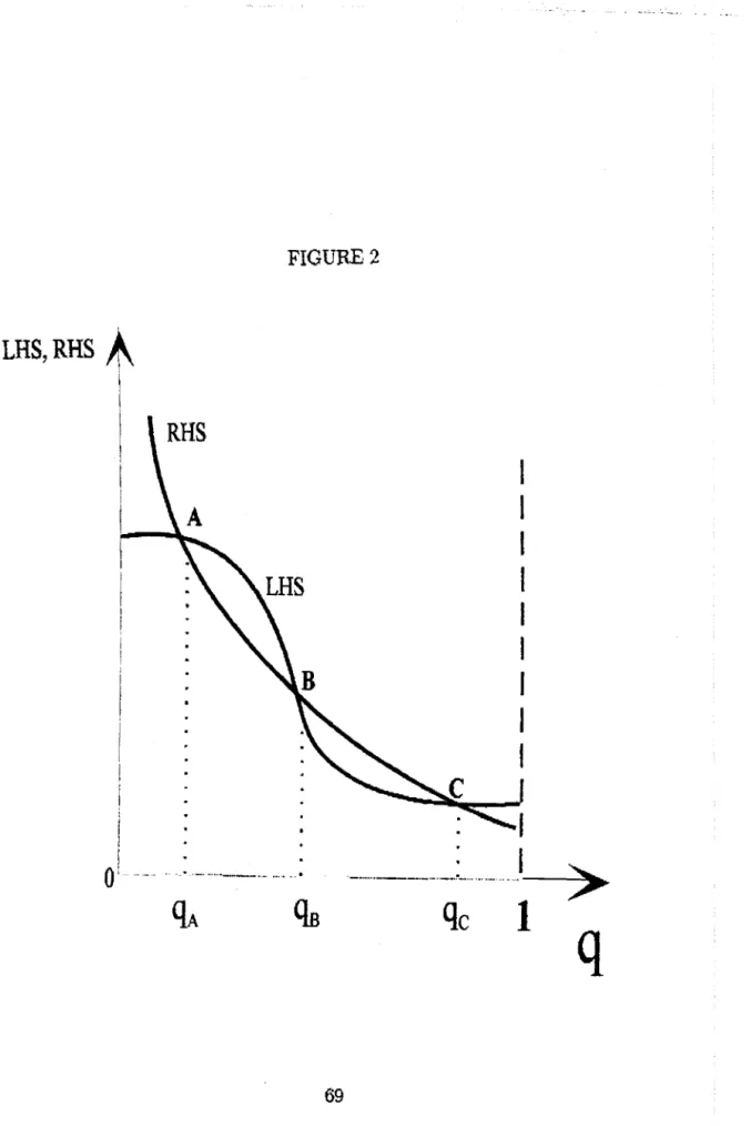
1. •The proof of proposition 3 in the appendix shows that the system of seven equations that characterize the stationary equilibrium can be reduced to a single equation, equation (25), with the unknwon variable q. The left-hand side (LHS) of this equation is equal to
,B'!f!(:r .,.,
where the denominator is the discount factor applied to the margina benefit of investment. The right-hand side (RHS) is the ratio of the current value of the marginal benefit of investment in education to the marginal benefit of consumption. In proposition 3, it is shown that this ratio declines with q, as drawn in figure 2. Using assumption 6, the LHS has the shape depicted in figure 2.1715In a later version of this paper, it will be computed solutions with different values for the parameters.
16 About this technological feature, Azariadis and Drazen writes: "Among the types of externalities we consider are spillovers from the stocks of different types of capital (to capture in a primitive way the notion of "infrastructure") as well as the labor-augmenting outcomes of externalities arising in the process of creating human capital."
FIGURE 2
LHS,RHS
A
I
o ... -... ----... .
qA
'la
69
:>
Looking at figure 2, we can see that there are multiple values for q that satisfies the equation that characterizes the stationary equilibria (equation(25)). In other words, it indicates that there are multi pIe balanced growth path. Each path is characterized by a different value for q: q = qA (equilibrium A),
q
=
qB (equilibrium B), and q=
qc (equilibrium C), where qA<
qB<
qc·Using the discussion above, we can compare the economic growth rate and income distribution in these different equilibria. The economy in equilibrium C, with the highest q, will grow faster with less inequality in comparison with economies in equilibrium A and B. The same is true for economy in B in comparison with one in A.I8 Therefore, one should not necessarily expect
alI countries to converge to the same economic growth as well as to the same income inequality.
The explanation for an economy to stay in a 'bad' equilibrium such as A runs as follows. An economy with a low quality labor force today is expected to grow slow. Agents with forward-Iooking behavior realize it and they are discouraged to invest in their child's human capital as the benefits of these investments are perceived to be low in such stagnant environment. This is true in despite of the great differences in income of skilled and unskilled workers (great income inequality). The slower the expected economic growth rate, the greater is the discount imposed by the present generation on future consumption, which is given by f3'IjJ(q) l-a . Hence, low expected growth rate
inhibits investments in human capital and the quality of the labor tomorrow,
q, turns out to be low again, maintaining the economy in an equilibrium with very unequal income distribution and low growth rates.
Note that the assumption of absence of markets to finance investments in education does not drive the above result of multiple balanced growth path. The crucial assumption to obtain this result is the 'threshold property'. If
this last assumption is dropped, equation (25) would be satisfied by only one value of q. That is, there would be only one stationary equilibrium.
5.2
Numerical Example
In order to show in proposition 3 that there exists at least one stationary growth path, we made the simplifying assumption that O
<
(J' =e
<
l.As mentioned above, this assumption implied that both types of agents invest the same fraction of their income in their offspring's education. The objective in this chapter is to use more commonly accepted paramater values in numerical examples and to make the above points more concrete. In particular, we want to consider examples in which the coefficient of relative
risk aversion, ()", is greater than one.
Values have to be chosen to six parameters in the model. There are two paramteres related to the individuaIs' preferences: the discount factor, {3,
and the coeificient of relative risk aversion, ()". There are two parameters associated with the production function: the multiplicative term, A, and a.
Finally, using the same probability function specified in assumption, there are the parameters k and (), which have to be between O and 1. In addition, a functional form for the learning by doing technology has to be specified.
The preference parameter, ()" = 1.5, is within the range of values com-monly used in real business cycle models.
We consider one period in this model to be equivalent to 30 years. As-suming an annual interest rate to be around 3% per year, we set the discount factor {3 = 004.
We follow Stokey (1996a) and consider a skilled worker to be one with at least a high school education. As pointed out by Stokey (1996a), "In 1985, 20% of the adult population in the V.S. had completed college, 13% had 1-3 years of college, 38% had completed high school, and 29% had not completed high school." Hence, we look for a stationary equilibrium in which
q is approximately equal to .71.
Stokey (1996a) points out that "in the V.S. over the period 1963-1989, the wages of college graduates, college dropouts, and high school dropouts relative to high school graduates were IA, 1.15, and 0.75." Weighting by the population proportions mentioned ab ove , she calculates the ratio of the skilled wage to the unskilled wage in the V.S. economy over this period to be 1.5. Thus, in the calculations below, we look for a stationary equilibrium in which :!!2b.. is approximately equal to 1.5.
Wl
In the theoretical framework, the learning by doing technology is the 'engine' of growth. Economic growth over the 30 years period is equal to 'lj; ( q) = [1
+
9 (AqQ)] .19 The quality oflabor force, q, will ultimately determine the growth rate. We specify the following functional form for the function g:g(
x) =A::-l'
This functional form satisfies the properties of the 9 functionin assumption 1. We set the parameter b equal to 1.24. It implies that the steady state GDP per capita growth over the 30 years period with the fraction of skilled workers in the economy equal to .71 (q = .71) fits the actual data for the V.S. The average GDP per capita growth of the V.S. economy over the period 1960-1990 was 2.1%.
The remaining parameters, a, (), k, and A are chosen such that the model's stationary growth path roughly fits the facts mentioned above. Therefore, the parameters values used in the computation are:
a = .3, () = .95, k = .93, and A = 100.
As pointed out ab ove , seven non-linear equations with seven unknows characterize the stationary equilibrium. We reduce it to a system with five equations and five unknows (q, Vz, Vh, Ez, Eh). The computer method used in
the numerical calculations in this paper is Newton's Method for Multivariate Equations.20 The calculated steady state values are:21
q - .7103, Vz = -.3408, Vh = -.2875,
Ez - .2682, Eh = .5641.
Consequently, the ratio !E.b.. is equal to 1.60.22
Wl
In the theoretical examination in the first part of this chapter, we showed that there is a possibility of multiple stationary equilibria. The path with higher economic growth rate would also be the one with a more egalitarian income distribution. We also showed that the crucial assumption to oh-tain this result is the imposition of a 'threshold' property in the technology with externality as used in Azariadis and Drazen (1990). The simplifying assumption O
<
a = ()<
1 was imposed in the theoretical analysis. Our objective now is to give a numerical example, using more accepted values for the parameters, to illustrate the possibility of multiple equilibria.In order to capture the 'threshold' property in the learning by doing technology, we assume the following: f37jJ(q)l-a = f3 if O
<
q::S
.3 andf37jJ(q)l-a '" 1 for .3
<
q<
1.23 This assumption implies that there would be no economic growth rate if there is any stationary equilibrium in which the fraction q is lower than .3. It also implies that the economic growth rate would be very high if there is any stationary equilibrium in which the fraction q is greater than .3.The parameters values used in the computation are:
f3
=
OA, a= 1.5,
A= 100,
k= .93, ()
= .7
and a= .9.
There are two set of steady state values that satisfies the five equations that characterizes the stationary equilibrium. The two steady state values for q are .2998 and .5711.24 It indicates that there are two stationary growth
20 Ali the calculations in this paper to obtain the steady state values use the same technique.
21 Next section, when we calculate the effects of government intervention on growth, income distribution and welfare, we use the stationary growth path associated with these steady state values as the benchmark case.
22The wages' steady-state values are: Wz
=
63.1725 and Wh=
101.2894.23Recali that the term fi'ljJ(q)l-(j is the "extended discount factor" which includes the discount factor fi, and the economic growth rate to the power (1 - 0"), 'ljJ(q)l-(j. In our numerical example, we make sure that fi'ljJ(l)l-(j < 1, as specified in assumption 4.
24The other steady state values are: (i) when q
=
.2998 - Ez=
.0916, Eh=
45.3609,Vz
=
-.6311, Vh=
-1.7525, Wz=
3.3815 and Wh=
104.9044; (ü) when q=
.5711 - Ez=
paths, with different growth rates and income distribution. As expected by the theory, the 'bad' equilibrium, with q
=
.2998, has lower economic growth rate and more unequal income distribution in comparison with the other equilibrium. As pointed out in the theoretical discussion, economic agents would not have great incentives to invest in their child's human capital when the expected economic growth rate is low. In the 'bad' equilibrium, the low and high type agents spend, respectively, 2.7% and 43% oftheir total income in their child's education. The correspondent numbers for the equilibrium with growth, when q = .5711, are 16% and 65%.6
Government intervention
There are two inefficiencies in this economy that justifies government in-tervention. First, there is no market to finance investment in education.25
With decreasing returns on this investment (-rrEE
<
O) and same ability for all members of the young generation (same 7r), the quality of the labor force(q) could be improved if the access to education becomes more equal. This equalization would occur with complete capital markets. Second, there are the externaI effects associated with the learning by doing technology. As mentioned above, each firm does not have any incentive to suffer any loss to accelerate learning because its piece of knowledge spills over instantly across the whole economy. In this model, the learning process can only be acceler-ated through an improvement in the quality of the labor force.26 Therefore,
a country's educational policy will be a crucial element to determine its economic path.
An efficient government intervention should focus on two aspects: equal-izing the access to education and improving the quality of the labor force. Intervention along these lines is one of the main explanations for the extraor-dinary economic performance with a relatively equitable income distribution of the East Asian countries. Since the sixties, the government of these coun-tries have focused their educational expenditures on primary and secondary education, where the capital market imperfections and information prob-lems are more severe. Public expenditures on tertiary education increased only in the last two decades after universal and near universal enrollment rates had been achieved at the primary and secondary leveIs and a shift in the structure of production toward more sophisticated and skill-intensive
25It seems realistic to assume that someone's education depends in great lenght on his parent's income.
•
•
products had occurred.27
In this chapter, we introduce two different educational policies with the objective to reduce the inefficiencies mentioned above. First, the government supplies vouchers that can only be used to finance education. Second, it offers public schools as an alternative to private schools. We then analyze the effects of this intervention on economic growth rate and income inequality.
6.1
Public
Schools
Government decides total expenditures in education per pupil who studies in public school, Eg. It imposes the same income tax rate (7) to all individuals to finance it.
The parent must opt for sending his child to public or private school. He pays taxes independently of his choice. If he chooses the first alternative, then his child will receive Eg units of investment in his education. If he picks the second alternative, he must decide how much to invest in his offspring's ed ucation. 28
The individual type x's problem with the option of public schools can be summarized by the following dynamic problem:
(19)
where:
such that:
PUx is the individual type x's utility if he chooses to send his child to
public school. The parent will consume his net income and Ex = O .
such that:
27See Page (1993).
P Rx is the individual type x's utility if he chooses to send his child to private school. His problem will be exactly equal to the environment without government intervention. The only difference is that he will pay taxes to finance public schools expenditures even sending his kid to private school.
In the above formulation, we limit the investments in education in some-one who goes to public school by Eg, an amount chosen by the government. One can imagine that a parent might want to invest additional amounts in tutoring and private classes to complement his child education. In this case, the parent's problem if he sends his child to public school would become:
such that:
Ex would be the additional investment. It is obvious that if faced with this alternative, the option private school (P R) would be a1ways inferior and max(PR, PU) = PU.
However, a student is required to spend many hours per day in a school, private or publico He can 'waste' significant hours of his day if he studies in a low quality school. In particular, if the quality of the public school is very low, additional expenditures in education may not guarantee a better education in comparison with a private school. Moreover, the option of a public school can turn out to be more expensive. The additional expendi-tures to give a public school student the same probability of becoming an individual with high leveI of human capital as a private school student may be enormous. Hence, a parent may prefer to send his child to private school and ignore the option of 'free' education. These are good explanations for the existence of private schools when public ones are available. To capture this possibility, we maintain from now on the earlier formulation in which the alternative to invest in education beyond Eg is not possible.
Definition 3: A recursive competitive equilibrium with public schools, given the initial condition qo, qo
E (0,1],
and {Eg}~o, is defined to be value functions v :[0,1]
x {x} -lo R, policy functions Cx :[0,1]
-lo R+,and Ix :
[0,1]
-lo R+, an economy-wide law of motion for the fraction ofindividuaIs with high leveI of human capital Q :
[0,1]
-lo[0,1],
and factorprices functions Wx :
[O, 1]
-lo R+ such that: (x E {h, I} ) (i) v satisfies the household problem (19);(iii) the wage functions are given by equations (8) and (9); (iv) the economy-wide law of motion for q is given by:
where Àx is the fraction of the young generation whose parents are
type x who goes to study in public schools, and À = Àh
+
ÀI ;(v) the government budget is in equilibrium:
The definition of stationary equilibrium with public schools is exactly equal to the one without it. Again, we confine our analysis to balanced growth equilibrium.
Note that if the government expenditures in education per pupil (Eg) is low enough, alI parents will send their children to private school, i.e., À = O. Such equilibriurn will be exactly equal to the one in chapter 4, without government intervention.
Proposition 4: With the introduction of public schools, there is an Eg
such that the fraction of skilled workers, q, is greater than the one in the equilibrium without public schools. •
The above proposition says that, by introducing public school, the gov-ernment can induce the whole society to invest a greater amount in edu-cation. It wiIl lead to an improvement in the quality of the labor force (greater
q)
and, ultimately, to a better economic performance and less in-equality. This wiIl happen in spite of the distortion caused by the income taxo Private investments in education wiIl be discouraged because of the negative wealth effect implied by the income taxo It will also be discouraged by the reduction in the differences in income between low and high types caused by the increase in the quality of the labor force.Proposition 5: With the introduction of public schools, there is an Eg
such that the fraction of skilled workers, q, is lower than the one in the equilibrium without public schools . •
families would be discouraged to invest in education due to the negative wealth effect related to the income taxo The result is that the whole society would invest less in education. The consequence is a reduction in the quality of the labor force (q), lower economic growth and more inequality.
6.2
Numerical Example with Public Schools
To make the above points more concrete, we provi de a few examples. The objective here is to calculate the steady state values of the utility leveIs of both types of agents as well as the fraction of workers with the high leveI of human capital in the stationary equilibria with different leveIs of government expenditures in public school. The next step is to compare them with the correspondent values in the equilibrium without public schools. Finally, the numerical examples are expected to support the theoretical results obtained in propositions 4 and 5.
The first equilibrium computed in chapter 5.2, without public schools, is used here as a benchmark. The steady state values of this equilibrium is reproduced in the first column of table 1. The same calibration specified in this benchmark case is used throughout this chapter.
The first experiment is to set government's expenditures per pupil in public school to be 10% greater than the amount the low type agent spends in their child's education in the benchmark case [Eg = (l.l)ErJ. The new steady state equilibrium is reported in the second column of table 1. The fraction ofworkers with high leveI ofhuman capital (q) increases .08%, from
.7103 to .7109. Consequently, the annual GDP per capita growth increases slightly from 2.1279% to 2.1299%. Moreover, both type of agents are better off as a result of this intervention. The utility leveIs of the high and low type agents augments from -.2875 and -.3408 to, respectively, -.2874 to
- .3401. It indicates that this policy is Pareto improving.
In the second experiment, government's expenditures per student in pub-lic school corresponds to 20% greater than the amount spent in education by the low type agent in the benchmark case [Eg = (1.2)ErJ. The results are reported in the third column of table 1. As in the first experiment, the fraction q jumps. It goes from .7103 to .7118. The new annual GDP growth rate would be 2.1313%, greater than the rate 2.1279% without public schools. In addition, as in the first experiment, this greater increase in the quality of public schools is still Pareto improving in comparison with the benchmark case. The utility leveIs of the high and low type agents increases from -.2875 and -.3408 to, respectively, -.2874 to -.3400.
in-creases from -.3401 to -.3400, whereas the high type agent's utility remains unaltered at - .2874.
The above experiments confirm, as expected, the theoretical result ob-tained in proposition 4: the introduction of public schools can move the economy to an equilibrium with higher growth rates and lower inequality. As discussed in the above in the theoretical examination, a greater q implies a lower Gini coefficient, i.e., less inequality.
Finally, we introduce public schools in which the government spends per student only 80% of the amount spent in education by the low type agent in the equilibrium without the option of public schools. The results are reported in the last column of table 1. There is a reduction in q. It drops from .7103 to .7079 in comparison with the benchmark case. It represents a reduction in the GDP per capita growth rate from 2.1279% to 2.1225%. This numerical example supports the theoretical result obtained in proposition 5. Low type agents would prefer, in this case, to take advantage of the 'free' public school system, invest less in their child's human capital and benefit from more consumption. Their utility leveI would increase from - .3408 to -.3406. In contrast, high type agents would be worst off with a reduction in utility from - .2875 to .2876.
Eg =0
.7103 -.3408 -.2875
O
6.3
VouchersTable 1
Eg
=(1.1)Er
.7109 -.3401 -.2874 .0009Eg
=(1.2)Er
.7118 -.3400 -.2874.001
Eg
=
(0.8)Et
s.7079 -.3406 -.2876 .0007
Government decides to transfer resources in the form of vouchers (T) that can be used exclusively to finance education. The recipients of these vouchers can be restricted to a specific group in the society or noto Again, it imposes the same income tax rate (T) to alI individuaIs to finance it.
A parent receives vouchers or not and decide how much to invest in his child's education. He is not restricted to invest only the vouchers in his offspring's education but he is obliged to invest at least that amount.29
29 As it is assumed that public and private schools have the same probability function
7r, it does not matter if we allow parents to use vouchers in public schools and private
The individual type x's problem with vouchers can be summarized by the following dynamic problem:
such that:
and
J.lx is an indicator function:
{ = 0,
= 1,
if the government does not supply vouchers to families whose parents are type ~
if the government does supply vouchers to families whose parents are type x.
Definition 4: A recursive competi tive equiIibrium with vouchers, given
the initial condition qo, qo E (O, 1], {T}~o, and {J.lx}~o, is defined to be vaIue functions v :
[0,1]
x{x}
~ R, policy functions Cx :[O, 1]
~ R+,and Ix :
[O, 1]
~ R+, an economy-wide law of motion for the fraction of individuaIs with high leveI of human capital Q :[O, 1]
~[0,1],
and factor prices functions Wx :[O, 1]
~ R+ such that: (xE
{h, I} )(i) v satisfies the household problem (20);
(ii) Cx and Ix are the optimal policy functions for (20); (iii) the wage functions are given by equations (8) and (9); (iv) the economy-wide Iaw of motion for q is given by:
(v) the government budget is in equiIibrium:
The definition of stationary equilibrium with vouchers is exactly equal to the one without it. Again, we confine our analysis to balanced growth equilibrium. In order to prove the following proposition, we assume that
I/. - I/. - 130
,...,l-,...,h- .
Proposition 6: With the introduetion of vouehers, there is a T sue h that the fraetion of skilled workers, q, is greater than the one in the equilibrium without vouehers . •
The results obtained with public schools are replicated with vouchers. It indicates that both types of intervention are equivalent, at least theoretically. As in the public school case, the government through vouchers can force the whole society to invest a greater amount in education. It will also lead to an improvement in the quality of the labor force (greater
q)
and, ultimately, to a better economic performance and less inequality.6.4 Numerical Example with Vouchers
The analysis in this section is similar to the one performed in section 6.2. The objective here is to calculate the steady state values of the utility leveIs of both types of agents as well as the fraction of workers with the high leveI of human capital in the stationary equilibria with different leveIs of govern-ment expenditures in vouchers. Another objective is to compare them with the correspondent values in the equilibrium without vouchers. Finally, the numerical examples are expected to support the theoretical result obtained in proposition 6.
The results obtained in the benchmark case, without vouchers, is repro-duced in the first column of table 2. As in the numerical example with public schools, the same calibration specified in this benchmark case is used throughout this chapter.
Two experiments are performed in this chapter. In the first one, the gov-ernment distributes vouchers to alI families with the face value 10% greater than the amount the low type agents spend in their child's education in the benchmark case
[(l.l)Erl.
In the second experiment the amount is 20%greater
[(1.1)EZSl.
31 The results are reported, respectively, in the second and last columns of table 2.In the first experiment, the fraction q moves from .7103 to .7112. Thus, the annual GDP per capita growth rate increases from 2.1279% to 2.13%.
As in the similar experiment with public schooIs, this introduction of the vouchers system is also Pareto improving. The utility leveIs of the high and low type of agents augments from - .2875 and - .3408 to, respectively,
-.2871 and -.3400.
Similar qualitative results are obtained in the second experimento The fraction q moves from .7103 to .7120, representing an increase in the annual GDP growth rate from 2.1279% to 2.1318%. The utility leveI of both types