DOMESTIC CONSUMPTION IN ROMANIA
DANIEL BELINGHER, Ph.D.
INSTITUTE FOR ECONOMIC FORECASTING, ROMANIAN ACADEMY
[email protected]
Abstract
“What drives government bonds?” or “what are the forces which are staying behind the yield of these bonds?” are questions, which are concerning both theoreticians and practitioners nowadays. This paper analyzes the way in which the domestic consumption, represented through households’ consumption, in Romania, is able to move the sovereign bond yield for the same country, on a short horizon. In order to do this, we have used in the current study, an autoregressive vector – VAR(1), in which are included the two mentioned variables. The analyzed period starts in 2008 (q1), it ends in 2012 (q3) and the used data is expressed quarterly.
Key words: : households’ consumption, bonds yield, autoregressive vector. JEL Code: E03, E21, G12, G32.
1. Introduction
–
Sovereign Bonds
The idea of writing this paper came after reading on Federal Reserve Bank of San Francisco’s website the article entitled “What makes the Yield Curve Move”, written by Tao Wu (2003). Also, my main research interest during the last year was the ricardian equivalence and the state bonds issue, which is directly linked to this field. A secondary slope in starting this paper was the analysis of Vamvoukas et al. (2008), regarding the test on the ricardian equivalence on Greece, in which one year bond rates is taken as a variable in testing the above mentioned hypothesis.
Based on the field of interest, this paper presents an econometric model for the Romanian economy. The model consists in a first order autoregressive vector with two variables – VAR (1). The variables that will were taken into consideration in the current research are the households’ final consumption and Romania’s 1-year bond yield. The logic and the main reasons behind choosing these two macroeconomic variables, are detailed further, in the second section of the current paper. As far as we have studied the related literature, this represents one of the first attempts of formalizing this kind of relation for the Romanian economy.
“What drives government bonds?” or “what are the forces which are staying behind the yield of these bonds?” are questions, which are concerning both theoreticians and practitioners nowadays. Because of the last years’ financial crisis, there was a massive migration of the capitals from higher risk destinations to lower risk destinations. One of these destinations, having in mind the risk aversion background, can be considered sovereign bonds.
According to the Swiss National Bank’s, there are five major drivers for the government bonds yields:
a) Inflation and inflation expectation, being by far the most important criterion. High inflation expectations are usually followed by higher bond yields and the main force behind these expectations is the wage evolution;
b) Wealth of a country is negative correlated with the government bond yields;
c) Interventions of the central banks (quantitative easing may be an example);
d) Foreign debt as a percentage of GDP;
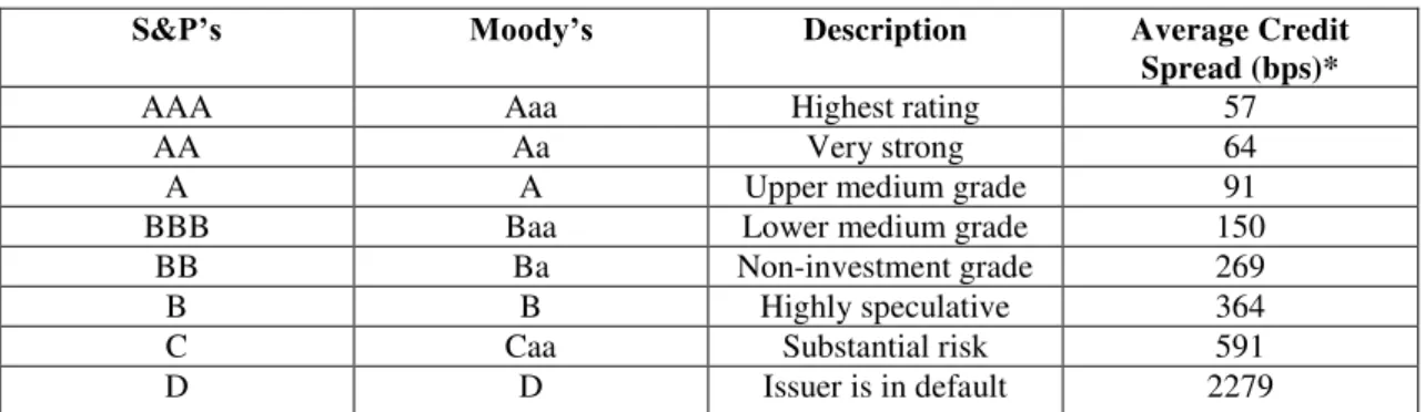
Table 1. Bond Rating Scale
S&P’s Moody’s Description Average Credit
Spread (bps)*
AAA Aaa Highest rating 57
AA Aa Very strong 64
A A Upper medium grade 91
BBB Baa Lower medium grade 150 BB Ba Non-investment grade 269
B B Highly speculative 364
C Caa Substantial risk 591
D D Issuer is in default 2279
* Source Barclays as if 12/31/2013 Source of the table: www.nasdaq.com
In Europe, since the crisis started, the launch of ECB quantitative easing policies exerted an influence on the credit risk between 73.78% and 86.58%, for the following countries: Romania, Bulgaria, Austria, Ukraine, Hungary, Poland, Germany, Russia and Turkey (Albu et al., 2014a). Similar results have been reported in Albu et al. (2014b).
2. Related Literature
The main research hypothesis followed in this paper it is directly linked to the ricardian equivalence hypothesis (R.E.H.) and, questions the linkage between the domestic consumption and bond yields. Various authors, such as Barro (2006), Barro and Ursua (2008) or Nakamura et al. (2013) are following the strength of this linkage, but from a different perspective: the one of the shocks (from financial crisis to natural disasters), which are affecting the output or the consumption and the correspondent peak-drop in yields. Nakamura et al. (2013) is analyzing the asset-pricing implications when a consumption shock occurs. In the three analyzed scenarios, from the previous mentioned paper, a sudden decrease in consumption causes a sudden decrease in the yields of stocks (1st scenario), U.S. treasury bills (2nd scenario) or long-term bonds (3rd scenario). The main difference between
the evolution of stocks or U.S. treasury bills compared to the one of the long-term bonds is that the decline in the corresponding yields is smaller than the one of the first category. This process is caused by the fact that the long-term bonds are considered and used as a tool for hedging in front of the “disaster risk”. The conclusion of this study was that it could be used as a guideline in consumption prediction only for the disaster periods. For the normality periods, it’s predictability power for future consumption growth is around 0% (R-squared = 0.03).
How does an asset price is formed? As the modern asset pricing theory is explaining, the core of this process consists in the fact that “assets are priced such that, ex-ante, the loss in marginal utility incurred by sacrificing current consumption and buying an asset at a certain price is equal to the expected gain in marginal utility contingent on the anticipated increase in consumption when the asset pays off in the future” (Mehra, 2001). Standard consumption-based asset pricing models are Rubinstein (1976), Lucas (1978), Grossman and Shiller (1981) and Hansen and Singleton (1983).
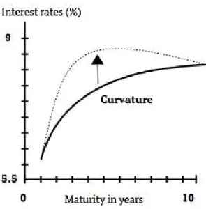
Fig. 1. Curvature in yield curve
Source: the author1
The relation between the consumption and the yield curve can be a double-sensed one, depending on the economy. Studies, like Harvey (1989), showed that yield curve measures have the potential to explain more than 30% of the variation in the rhythm of output (for 1953-1989 period for the US economy), compared to the stock market which is able to explain only 5% from this variation. Irving Fischer formalized the correlation between asset markets and the real economic growth, for the first time. He showed that “in equilibrium, the one-year interest rate reflects the marginal value of income today in relation to its marginal value next year” (Harvey, 1989). Zuliu Hu (1993) discovered that, after an analysis over the G-7 group of countries, “a simple measure of the slope of the yield curve, namely the yield spread, serves as a good predictor of future economic growth”.
3. Used Data
The model aggregates two macroeconomic variables. These variables are:
Households’ Final Consumption in Romania– source: Eurostat
Romania 1-Year Bond Yield – source: www.investing.com
The frequency of the used data is quarterly. The first time series was inflation adjusted, using as a base year for the inflation, the year 2005. By visually analyzing the time series for the households’ consumption, we have decided that the best thing will be to seasonally adjust the data, in order to have a higher accuracy of the model. The Romanian households’ consumption has a very pronounced cyclic component, as it can be seen from the following graph. As Sims (1993) concluded in his paper that, even the use of unadjusted data may be the best alternative, sometimes, treating seasonality can be a “nuisance” and can lead to worse errors than those produced by the usage of adjusted data. The following figure shows the differences between the seasonally adjusted series and non-adjusted series:
1
Adapted
after
Graph
C.
from
Fig. 2. Seasonally adjusted data vs. non-seasonally adjusted data (households’ final consumption in Romania)
Source of the data processed: Eurostat
We have transformed, also, the seasonally adjusted series into a natural logarithm (log) series for stabilizing the variance (Michener, 2003). The second time series did not suffer any transformation. For simplicity, we are going to use as acronyms for the time series, the following notations: logHHC (for households’ consumption)
and YBR (Romanian 1-Year Bond Yield).
The analyzed period starts in 2008q1 and it ends in 2012q3. Unfortunately, there are only 19 observations because of the low availability of the data for, the YBR series before 2008 and for HHC, after 2012. This is caused by the fact that the Romanian economy is a young economy, which just joined the European Union in 2007, and the calculus methodology changed very often or the data was not reported every time or in time by the local authorities.
4. Methodology and Estimates
In order to achieve our goal and build an econometric model, we have first tested the stationarity of the data. According to the tests, we have concluded that the data are stationary. A second phase in our research, was to estimate the number of lags, which are going to be used in the model. According to the pre-estimation tests results, in STATA, we have chosen a 1storder VAR model. Test’s result can be seen in the following table:
Table 2. Lag order selection test (pre-estimation)
as the Johansen test:
(1)
, where:
Xt is a vector of variables, (1- L) is the first difference operator; is a constant vector; is coefficient
matrix with reduced rank r<k and is a vector of innovations.
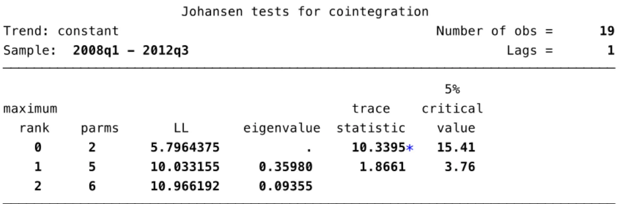
The results of the Johansen co-integration test, applied in STATA, can be found in the following table:
Table 3. Johansen co-integration test
Source: the author
According to the previous test, according to the trace statistic, we have decided that a VECM cannot be implemented, due to the lack of co-integration over the long run of the data series. As a consequence, a VAR model is better suited. A vector autoregression follows the below reduced form:
(2)
The corresponding matrix for a VAR (1) model would be:
= (3)
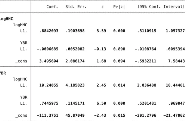
A table with the current VAR (1) model’s estimates, can be found further:
Source: the author
As it can be seen, the correlation of determination for the second equation, the one which presents interest for our research, is R-squared = 0.8. This value is showing as that, on the short-run, 80% of the variation of the yield for Romanian 1-year bonds is explained by the households’ final consumption. Also the probability value, for the first equation, the one directly studied in this research, is within the confidence interval (P<0.05). This means that the equation presents statistical significance.
There were made also tests for autocorrelation of the errors (Lagrange multiplier test) and error’s distribution. One can see from the below tests (table no. 5) that it does not exist errors’ autocorrelation and the errors are normally distributed, so the VAR model doesn’t violate the assumption of the classical model. Also, a stability test, for the VAR model has been realized and the model satisfies stability condition.
Table 5. VAR tests
in which the variable YBR (Romania 1-Year Bonds Yield) is endogenous (the second equation in table 4). The estimates of this equation can be rewritten as:
(4)
This equation shows that there is a positive linear correlation between, the Romania 1-Year Bonds Yield, the same variable in a previous period and the final households’ consumption in the t-1 period. Also the constant (-111.375) of this equation is statistically significant.
5. Impulse Response Function Analysis
According to Eigenvalue stability condition of the model, we can proceed to the next step. In order to this, in this section, we will analyze the Impulse-Response Function of the established VAR (1) model.
An Impulse-response function can be represented as:
(5)
and it offers the response of yit+nto a one-time impulse in yj,t with all other variables dated t or earlier held
constant.
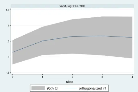
A shock was created in households’ final consumption in Romania, by using the IRF variable, as it can be seen in fig. 4, in order to see the response of the yield curve. The shock was applied over a period of 4 quarters, until the bond reaches the maturity. The orthogonalized IRF has a positive slope, so this means that if a shock in consumption occurs when the bond is issued, it will have a positive impact over the whole lifespan of a bond, until it reaches it’s maturity.
Fig. 4. VAR’s model IRF (Impulse: Households’ Consumption; Response: 1-Year Bonds Yield) – 4 steps
Source: the author
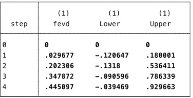
Table 6. Cholesky forecast-error variance decomposition
Source: the author
6. Concluding Remarks
We have shown through a VAR(1) econometric model that there is a link between a shock in the households’ final consumption and 1-Year Bonds Yield for the Romanian economy. Even though it is a very simple analysis and probably more factors should be added to the mentioned model, it can give us a hint regarding one of the most influential factors, which can move bonds’ yield curve in Romania: the households’ consumption. So in order to this, if a consumption shock occurs in the early life stages of a 1-Year Bond, this will manifest a positive influence over the whole’s bond lifespan. Also, the influence of a positive shock in households’ consumption will be also positive and its influence over time is increasing until the second quarter and it stabilizes at an upper limit, in the third and the forth quarter. Our empirical findings are inline with the related literature, in which other authors’ findings come to sustain that a shock in output or in domestic consumption can have a clear impact on an asset yield.
Acknowledgment. This work was supported by the project “Excellence academic routes in doctoral and postdoctoral research - READ” co-funded from the European Social Fund through the Development of Human Resources Operational Programme 2007-2013, contract no. POSDRU/159/1.5/S/137926.
7. References
[1] Albu, L. L., Lupu R., Călin C., Popovici O., (2014). “Estimating the Impact of Quantitative Easing on
Credit Risk through an ARMA –GARCH Model”, Romanian Journal of Economic Forecast 3(2014): 39-50. [2] Albu, L. L., Lupu R., Călin C., Popovici O., (2014). “A Nonlinear Model to Estimate the Long Term Correlation Between Market Capitalization and GDP per capita in Eastern EU Countries”, Working Papers of Institute for Economic Forecasting 141115.
[3]Ang, A., Piazzesi, M., (2001). “A No Arbitrage Vector Autoregression of Term Structure Dynamics with Macroeconomic and Latent Variables”, working paper 8363, National Bureau of Economic Research
[4]Augustin, P., Tedongap R., (2011). „Sovereign Credit Risk and Real Economic Shocks”, paper available on
http://www.eea-esem.com/files/papers/eea-esem/2012/1934/AT-CDS-December2011.pdf
[5] Bodislav A., (2014). „Transferring Business Inteligence and Big Data Analysis from Corporations to
Governments as a Hybrid Leading Indicator”, paper presented during „Post Crisis Developments” held by Bucharest University of Economic Studies in November, 21 2014.
[6] Campbell, J., (2003). „Handbook of Economics and Finance” edited by G.M. Constantinides, M. Harris and R. Stulz, Elsevier Science B.V.
[7] Cochrane, J.,(2001). „Asset pricing”, Princeton: Princeton University Press.
Evans, C., Marshall, D., (2006). “Economic Determinants of the Nominal Treasury Yield Curve”, Journal of Monetary Economics 54:7: 1986-2003.
Aggregate Fluctuations? American Economic Review: 249-71.
[10] Grossman, S.J., Shiller, R.J., (1981), “The determinants of the variability of stock market prices”, American Economic Review 71:222−227.
[11] Hansen, L.P., Singleton, K.J.,(1983), “Stochastic consumption, risk aversion, and the temporal behavior of asset returns”, Journal of Political Economy 91:249−268.
[12] Hu, Z., (1993), “The Yield Curve and Real Activity”, IMF Staff Papers 40(4): 781.
[13] Lucas Jr, R.E., (1978), “Asset prices in an exchange economy”, Econometrica 46:1429−1446.
[14] Lupu, R., Călin, C., (2014)“A mixed frequency analysis of connections between macroeconomic variables and stock markets in Central and Eastern Europe”, Financial Studies 18(2): 69 – 79.
[15] Marcet, A., (2004), “Overdifferencing VAR’s is OK”,paper prepared for seminar at CEMFI
[16] Mehra, R., (2001), “The Equity Premium: Why is it a Puzzle?”, draft from May 6, 2001, available on
http://www.econ.ucsb.edu/~mehra/puzzlepaper.pdf
[17]Mitcher, R. (2003), “Notes on logarithms” course notes available on:
http://people.virginia.edu/~rwm3n/pdf/Notes%20on%20logarithms.pdf
[18] Nakamura, E., Steinsson, J., Barro, R., Ursua, J., (2013), “Crises and Recoveries in an Empirical Model of Consumption Disasters”, American Economic Journal: Macroeconomics, 5(3): 35-75.
[19] Rubinstein, M., (1976), “The valuation of uncertain income streams and the pricing of options”, Bell Journal of Economics 7:407−425.
[20] Sims, Ch., (1993), “Rational expectations with seasonally adjusted data”, Journal of Econometrics 55(1993): 9-19.
[21] Vamvoukas, G., Gargalas, V.N., (2008), “Testing Keynesian Proposition And Ricardian Equivalence: More Evidence on The Debate”, Journal of Business and Economic Research Vol. 6 (5): 67-76
[22] Wu, T.,(2003), “What Makes the Yield Curve Move”, Economic Letters of Federal Reserve Bank of San Francisco available on: http://www.frbsf.org/economic-research/publications/economic-letter/2003/june/what-makes-the-yield-curve-move/
[23] *** “Bond Basics: Corporate vs. Sovereign Risk” available on: http://www.nasdaq.com/article/bond-basics-corporate-versus-sovereign-risk-cm326211