doi:10.5194/acp-12-2881-2012
© Author(s) 2012. CC Attribution 3.0 License.
Chemistry
and Physics
Satellite constraint for emissions of nitrogen oxides from
anthropogenic, lightning and soil sources over East China on a
high-resolution grid
J.-T. Lin
Laboratory for Climate and Ocean-Atmosphere Studies, Department of Atmospheric and Oceanic Sciences, School of Physics, Peking University, Beijing 100871, China
Correspondence to:J.-T. Lin ([email protected])
Received: 28 September 2011 – Published in Atmos. Chem. Phys. Discuss.: 7 November 2011 Revised: 10 March 2012 – Accepted: 13 March 2012 – Published: 23 March 2012
Abstract.Vertical column densities (VCDs) of tropospheric nitrogen dioxide (NO2) retrieved from space provide valu-able information to estimate emissions of nitrogen oxides (NOx) inversely. Accurate emission attribution to individ-ual sources, important both for understanding the global bio-geochemical cycling of nitrogen and for emission control, remains difficult. This study presents a regression-based multi-step inversion approach to estimate emissions of NOx from anthropogenic, lightning and soil sources individually for 2006 over East China on a 0.25◦long×0.25◦lat grid, employing the DOMINO product version 2 retrieved from the Ozone Monitoring Instrument. The inversion is done gridbox by gridbox to derive the respective emissions, tak-ing advantage of differences in seasonality between anthro-pogenic and natural sources. Lightning and soil emissions are combined together for any given gridbox due to their similar seasonality; and their different spatial distributions are used implicitly for source separation to some extent. The nested GEOS-Chem model for East Asia is used to simulate the seasonal variations of different emission sources and im-pacts on VCDs of NO2for the inversion purpose. Sensitivity tests are conducted to evaluate key assumptions embedded in the inversion process. The inverse estimate suggests annual budgets of about 7.1 TgN (±39 %), 0.21 TgN (±61 %), and 0.38 TgN (±65 %) for the a posteriori anthropogenic, light-ning and soil emissions, respectively, about 18–23 % higher than the respective a priori values. The enhancements in an-thropogenic emissions are largest in cities and areas with ex-tensive use of coal, particularly in the north in winter, as ev-ident on the high-resolution grid. Derived soil emissions are consistent with recent bottom-up estimates. They are less than 6 % of anthropogenic emissions annually, increasing to about 13 % for July. Derived lightning emissions are about 3 % of anthropogenic emissions annually and about 10 % in
July. Overall, anthropogenic emissions are found to be the dominant source of NOxover East China with important im-plications for nitrogen control.
1 Introduction
Nitrogen oxides (NOx≡NO + NO2) are important con-stituents in the troposphere affecting the formation of ozone and aerosols with significant consequences on air quality, cli-mate forcing and acid deposition. They are emitted from an-thropogenic combustion sources as well as natural sources from lightning, soil and biomass burning. Understanding the individual contributions of anthropogenic and natural emis-sions is critical both for evaluating the effects of NOx on the global environment and for forming appropriate emission control strategies in polluted areas like East China.
Several inversion studies have attempted to separate an-thropogenic from other sources of NOx, especially soil sources, based on measurements from the Global Ozone Monitoring Experiment (GOME) instrument (Jaegl´e et al., 2005; M¨uller and Stavrakou, 2005; Wang et al., 2007; Stavrakou et al., 2008), the Scanning Imaging Absorption Spectrometer for Atmospheric CHartographY (SCIAMACHY) instrument (M¨uller and Stavrakou, 2005; Stavrakou et al., 2008), and the Ozone Monitoring Instru-ment (OMI) (Zhao and Wang, 2009). Jaegl´e et al. (2005) and Wang et al. (2007) proposed two different methods to separate anthropogenic, soil and biomass burning emissions month by month with no attempt to constrain lightning emis-sions. Jaegl´e et al. (2005) assumed the a posteriori non-lightning emissions to be solely anthropogenic if the a pri-ori anthropogenic emissions exceed 90 % of the a pripri-ori to-tal emissions or if they exceed the a posteriori non-lightning emissions. Otherwise, differences between the a posteriori and a priori emissions were attributed to soil or biomass burning sources. A similar criterion was adopted by Zhao and Wang (2009) to differentiate anthropogenic and soil emissions. Wang et al. (2007) distinguished anthropogenic and soil sources using prescribed values for errors in the a priori anthropogenic emission data. Specifically, if the a pos-teriori non-lightning non-biomass burning emissions exceed the a priori anthropogenic emissions plus errors (assumed to be 40–60 %), the differences are attributed to soil sources. M¨uller and Stavrakou (2005) and Stavrakou et al. (2008) used an adjoint modeling approach for source attribution. Wang et al. (2007) suggested that soil emissions over East China amounted to 0.85 TgN per year for 1997–2000, differ-ing significantly from other inverse estimates (Jaegl´e et al., 2005; M¨uller and Stavrakou, 2005; Stavrakou et al., 2008; Zhao and Wang, 2009; L. Jaegl´e, personal communication, 2011; C. Zhao and Y. Wang, personal communication, 2011). Soil emissions derived from the inverse modeling also dif-fer from the bottom-up estimates (Yienger and Levy, 1995; Yan et al., 2003, 2005; Hudman et al., 2012; Steinkamp and Lawrence, 2011); in particular, they are 50–300 % larger than the Yienger and Levy (1995) estimate. According to Jaegl´e et al. (2005) and Wang et al. (2007), soil emissions may be as large as 40–50 % of anthropogenic emissions in summer for East Asia in 2000 and for East China in 1997–2000, re-spectively, with significant implications for the global bio-geochemical cycling of nitrogen.
The magnitude of lightning emissions is difficult to es-timate (Boersma et al., 2005; Schumann and Huntrieser, 2007), especially on the regional scale with significant vari-ations in lightning occurrences from one year to another (Schumann and Huntrieser, 2007). Most inverse estimates did not attempt to constrain lightning emissions (Jaegl´e et al., 2005; Wang et al., 2007; Zhao and Wang, 2009; Lin et al., 2010a, b; Lin and McElroy, 2010). The inverse model-ing by Stavrakou et al. (2008) suggested lightnmodel-ing emissions to be 50–80 % larger than their a priori values (3 TgN yr−1
globally) with the largest difference over the tropics; the study did not specify the magnitude of lightning emissions over China.
This study presents a new method to inversely derive emissions of NOx for 2006 over East China (101.25◦E– 126.25◦E, 19◦–46◦N; see Fig. 1) from anthropogenic, light-ning and soil sources individually based on satellite re-trievals of NO2columns and simulations of the global chem-ical transport model (CTM) GEOS-Chem. Emissions from biomass burning are not constrained since they are unimpor-tant over East China (Wang et al., 2007; Lin et al., 2010a). A regression-based multi-step inversion approach is used to derive emissions for all months, exploiting information on the seasonal variations of individual sources simulated by the CTM. The satellite data are taken from the DOMINO product version 2 (DOMINO-2) retrieved by the Royal Netherlands Meteorological Institute (KNMI) from the Ozone Monitor-ing Instrument (OMI) (Boersma et al., 2007, 2011). The nested GEOS-Chem model for East Asia (Chen et al., 2009) is used to calculate VCDs of NO2 in response to vari-ous emission sources for the inversion purpose. The top-down emissions are derived at a relatively fine resolution of 0.25◦long×0.25◦lat allowing for a more detailed analysis of the spatial distribution of emissions, compared to previ-ous studies (Jaegl´e et al., 2005; M¨uller and Stavrakou, 2005; Wang et al., 2007; Stavrakou et al., 2008; Zhao and Wang, 2009).
The paper is organized as follows. Section 2 presents the satellite product. Section 3 describes the CTM and com-pares simulated VCDs with retrieved values. Section 4 de-scribes the inversion process in detail and analyzes the re-sulting top-down emissions for anthropogenic, lightning and soil sources. It also evaluates the effects of key assumptions made during the inversion process. Section 5 presents the a posteriori emissions in comparison with previous inverse and bottom-up estimates. Section 6 concludes the present analysis.
2 VCDs of NO2retrieved from OMI
The KNMI DOMINO-2 product offers a level-2 dataset for VCDs of NO2 derived by three main steps involving the calculation of slant column densities (SCDs), tropospheric SCDs, and tropospheric VCDs (Boersma et al., 2007, 2011). The derivation relies on information on air mass factors (AMFs) to convert the tropospheric SCDs to VCDs. The AMFs are interpolated from a look-up table (LUT), and are subject to errors in the predetermined information for clouds, aerosols, surface albedo, the a priori vertical profile of NO2, surface pressure, and surface height. The reader is referred to Boersma et al. (2007, 2011) for detailed derivation of the product.
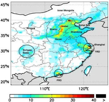
Fig. 1.Regional specifications with provincial boundaries for East China. Also presented are its subregions, provinces and province-level municipalities discussed in the text: the Yangtze River Delta (YRD), the Pearl River Delta (PRD), the Sichuan Basin, the Bo-hai Sea, Beijing (BJ), ShangBo-hai, Hebei, Henan, Shandong, Shanxi, Ningxia, Inner-Mongolia, and Sichuan. On the background is the annual mean VCDs of NO2from the DOMINO-2 product.
regions, and are mainly from the calculation of AMFs for polluted regions (Boersma et al., 2007). Compared to ver-sion 1, DOMINO-2 incorporates a variety of improvements on the LUT, surface albedo, and the a priori vertical pro-file of NO2(Boersma et al., 2011). It also includes a cross-track stripe correction and a high-resolution dataset for sur-face height. As a result, systematic biases found in ver-sion 1 are reduced significantly in DOMINO-2 (Boersma et al., 2011). The overall error for retrieved VCDs in DOMINO-2 is estimated to be about 30 % (a relative error) plus 0.7×10¹⁵molec. cm−2(an absolute error), likely with a magnitude larger in winter than in summer (Boersma et al., 2007, 2011; Lin and McElroy, 2010, 2011; Lin et al., 2010a). In this study, the relative error is assumed to vary nonlinearly from 30 % in summer to 50 % in winter based on the follow-ing formula: 0.3 + 0.2×(1−sin(i/10×π )), where i= 0, 1, 2, 3, 4, 5, 5, 4, 3, 2, 1, 0 for months from January to De-cember. This information will be employed for purposes of emission inversion; and the assumed seasonality will be eval-uated in Sect. 4.6.
In this study, the daily level-2 data from DOMINO-2 are gridded to 0.25◦long×0.25◦lat, which are averaged then to obtain monthly mean VCDs for subsequent emission in-version. The level-2 dataset includes measurements at 60 viewing angles corresponding to 60 ground pixels, and the pixel sizes increase nonlinearly from 13×24 km2 at nadir
to 25× ∼140 km2at the edges of the viewing swath. This study excludes pixels with cloud radiance fraction exceeding 50 % (Boersma et al., 2007). In addition, it only uses data from the 30 pixels around the swath center (with a cross-track length less than 30 km), allowing for a better analysis of the spatial distribution of VCDs within short distances. It consequently changes the swath width in use to about 800 km so that global coverage is achieved roughly about every three days. Note that the pixel sizes here are much smaller than the GOME (320×40 km2)and SCIAMACHY (60×30 km2)instruments used in previous inverse estimates (Jaegl´e et al., 2005; M¨uller and Stavrakou, 2005; Wang et al., 2007; Stavrakou et al., 2008).
3 Simulations of GEOS-Chem
3.1 Descriptions of model simulations
This study uses the nested model of GEOS-Chem (version 08-03-02; http://wiki.seas.harvard.edu/geos-chem/ index.php/MainPage) for East Asia run at a horizontal resolu-tion of 0.667◦long×0.5◦lat with 47 layers vertically (Chen et al., 2009). The model is run with the full Ox-NOx-CO-VOC-HOxchemistry. It is driven by the assimilated meteo-rological fields of GEOS-5 taken from the National Aero-nautics and Space Administration (NASA) Global Model-ing and Assimilation Office (GMAO). Vertical mixModel-ing in the planetary boundary layer follows the non-local scheme (Lin and McElroy, 2010) accounting for the varying magnitude of mixing from stable to unstable states of the boundary layer. Convection is parameterized based on a modified version of the Relaxed Arakawa-Schubert scheme by Moorthi and Suarez (1992) (Rienecker et al., 2008). The lateral boundary conditions are updated every 3 h using results from associ-ated global simulations at 5◦long×4◦lat horizontally.
Annual anthropogenic emissions of NOx, carbon monox-ide (CO) and non-methane volatile organic compounds (VOC) are taken from the INTEX-B dataset for 2006 pro-vided by Zhang et al. (2009), including sources from power plants, industry, transportation and the residential sector. Emissions from the residential sector are further assumed to vary month to month accounting for heating related emis-sions that depend on ambient air temperature (Streets et al., 2003). They, however, contribute only 6 % of anthropogenic sources of NOx on the annual basis (Zhang et al., 2009). Emissions from power plants, industry and transportation are held constant across the seasons since the seasonality is rel-atively small and is not included in the INTEX-B dataset. The impact of such simplification is found to be small (see Sect. 5). The diurnal variations of individual sources follow Lin et al. (2010a) and Lin and McElroy (2010, 2011).
(van der Werf et al., 2006); their magnitudes are negligible for NOxover China (Wang et al., 2007; Lin et al., 2010a) as the relatively low combustion temperature does not allow for significant production of NOx. In 2006, the emission budget for East China is only about 0.013 TgN.
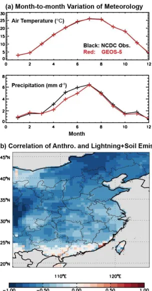
Production of NOx from lightning is determined by the flash rate multiplying the yield of nitric oxide (NO) from each flash. In GEOS-Chem, the NO yield is latitude de-pendent: over the Asian continent, the yield is set to be 500 moles per flash north of 35◦N reducing to 260 moles per flash south of 35◦N (Martin et al., 2006; Hudman et al., 2007), based on previous observational constraint that the NO yield in the tropics is lower than in the midlatitude (Huntrieser et al., 2006). The total (intra-cloud and cloud-to-ground) flash rate is determined by convective cloud top height to the 4.9th power over lands free of snow and ice, as formulated by Price et al. (1997). The total amount of lightning induced emissions is distributed vertically with a backward “C-shape” profile (Ott et al., 2010). Horizontally, as the flash rate depends on cloud properties that are highly parameterized, it is subject to large uncertainties particularly for individual locations. Alternate lightning parameteriza-tions based on cloud mass flux or convective precipitation (Allen and Pickering, 2002) were found not to improve the simulation of lightning distribution (Hudman et al., 2007). To improve the simulation, a horizontal adjustment is taken for each model gridbox based on the OTD/LIS satellite mea-surements of lightning flashes (Sauvage et al., 2007; Murray et al., 2009, 2010, 2012). For each month, the mean flash rate over 2004–2008 is set as the monthly climatology derived from the satellite measurements from 1995 to 2005; while the interannual variability is determined by the year-to-year varying cloud heights taken from the GEOS-5 meteorologi-cal fields (note that measurements for north of 35◦N are de-rived from the OTD instrument available in 1995–2000). The constraint on the monthly climatology is meaningful since no significant trend of lightning activities is found based on the satellite measurements (Sauvage et al., 2007; Murray et al., 2009, 2010, 2012). Over East China, convection and pre-cipitation amount are both driven by the seasonal transition of the East Asian Monsoon and thus are highly correlated month to month. Figure 3a shows that GEOS-5 captures the observed seasonal variation of precipitation and near-surface (2 m) air temperature, likely indicating that the seasonality of convection is simulated reasonably well, at least on the regional mean basis. It is expected thus that the season-ality of lightning activities is likely reasonably reproduced by GEOS-Chem, although large uncertainties still exist as-sociated with the exact magnitude and timing of lightning emissions.
Soil emissions are based on the Yienger and Levy (1995) scheme with the canopy reduction factors described by Wang et al. (1998). They include sources due to microbiological processes producing NOxnaturally as well as those associ-ated with use of chemical fertilizers and manure. The net
emissions vary with vegetation type (Olson, 1992), temper-ature and precipitation. The N-pulsing is determined by the amount of precipitation over lands containing dry soils prior to the precipitation (Yienger and Levy, 1995). It is noted that GEOS-5 simulates very well the seasonal variability of precipitation and air temperature (Fig. 3a). Fertilizer derived emissions are limited to agricultural lands and are distributed evenly over the growing season (May to August north of 28◦N and all year long in the tropics) (Yienger and Levy, 1995; Wang et al., 1998). They are assumed to be 2.5 % of the total amount of fertilizer use taken from the country based statistics of the Food and Agriculture Organization of the United Nations (FAO); for China, the fertilizer data rep-resent the year 1990 (Wang et al., 1998). As normally as-sumed, fertilizer associated emissions are considered to be part of natural sources in this study for comparison with an-thropogenic emissions relating to combustion.
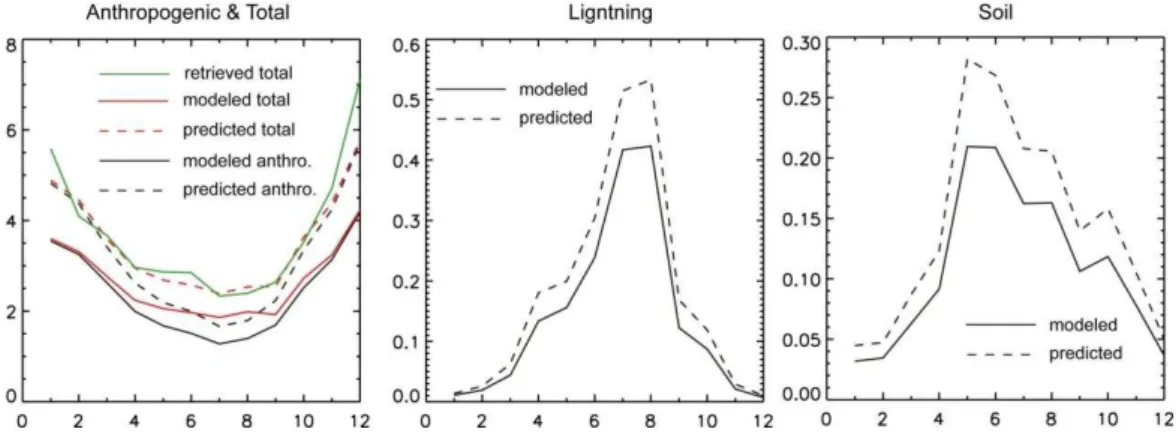
Averaged over East China, the a priori anthropogenic emissions of NOxare relatively constant across the seasons, while lightning and soil sources reach maximum values in summer and are not important in winter (Fig. 2). On the an-nual basis, the a priori anthropogenic emissions of NOxare about 5.8 TgN yr−1 over East China; and lightning and soil emissions are only about 3–6 % of anthropogenic emissions (Table 1). In July, lightning and soil emissions increase to as large as 10–13 % of anthropogenic emissions (Table 1). Locally, anthropogenic emissions exhibit a seasonal pattern that is negatively or weakly correlated with the seasonality of lightning and soil emissions (Fig. 3b). The spatial correla-tion between anthropogenic and lightning or soil emissions is lower than 0.36 in all months, with a value larger in summer and much lower in winter.
A total of five 1-yr simulations for 2006 were conducted to quantify VCDs of NO2from anthropogenic, lightning, soil and biomass burning sources, as shown in Table 2. For con-sistency with satellite retrievals, model VCDs in each day are obtained by regridding modeled NO2 at each vertical layer to 0.25◦long×0.25◦lat, sampled from gridboxes with valid satellite retrievals, and applied with the averaging ker-nel from DOMINO-2. The daily data are averaged then to obtain monthly mean values for each gridbox.
Fig. 2. Seasonal variations of the a priori, top-down and a posteriori anthropogenic, lightning, soil and total emissions of NOx
(1015molec. cm−2h−1)over East China for 2006.
Table 1.Emission budgets over East China (TgN) derived from various inversion calculations.
Case Description
Annual July
Anthro. Lightning Soil Anthro. Lightning Soil
A priori 5.763 0.174 0.324 0.479 0.0507 0.0627
Total errors in a priori emissions 60 % 100 % 100 % 60 % 100 % 100 %
1 Top-down (base case) 8.016 0.228 0.424 0.646 0.0623 0.0810
2 Use level-2 retrieval data from all 60 pixels 7.789 0.223 0.415 0.633 0.0616 0.0793 3 Re-allocate group 2 gridboxes to group 1 8.169 0.201 0.370 0.665 0.0529 0.0693
(and thus skip step 2 in Fig. 6)
4 Re-allocate group 2 and 3 gridboxes to 7.720 0.203 0.373 0.642 0.0534 0.0698 group 1 (and thus skip steps 2 and 4 in Fig. 6)
5 Assume constant retrieval errors across the seasons 8.306 0.220 0.400 0.668 0.0596 0.0754 6 Assume seasonality of anthropogenic emissions 7.830 0.259 0.480 0.640 0.0706 0.0911
according to Table 9 of Zhang et al. (2009)
7 Use soil emissions from Hudman et al. (2012) 7.876 0.202 0.506 0.636 0.0537 0.0797 8 Keep lightning emissions unchanged 7.950 0.174 0.645 0.644 0.0507 0.1145 9 Keep soil emissions unchanged 8.105 0.238 0.324 0.655 0.0657 0.0627 10 Shiftm,landm,sbackward by 1 month 8.029 0.212 0.375 0.641 0.0564 0.0702
11 Shiftm,landm,sforward by 1 month 8.001 0.204 0.397 0.641 0.0542 0.0756
12 Shiftm,lbackward by 1 month 7.991 0.222 0.401 0.636 0.0599 0.0757
13 Shiftm,lforward by 1 month 7.975 0.210 0.405 0.640 0.0559 0.0775
14 Shiftm,sbackward by 1 month 7.958 0.224 0.410 0.634 0.0614 0.0777
15 Shiftm,sforward by 1 month 7.943 0.226 0.423 0.627 0.0620 0.0803
16 Reduce magnitude ofm,landm,s 8.089 0.309 0.470 0.660 0.0835 0.108
17 Reduce magnitudes ofm,l 8.024 0.287 0.416 0.653 0.0772 0.0965 18 Reduce magnitudes ofm,s 8.075 0.242 0.462 0.652 0.0665 0.0887
19 Increase convection of anthropogenic NO2by 50 % 7.984 0.218 0.408 0.638 0.0595 0.0777
Sum in quadrature of percentage deviation of 7.2 % 58.3 % 67.9 % 7.4 % 58.1 % 68.7 % Case 2–19 relative to Case 1
Errors in top-down emissions due to assumptions 12.3 % 59.1 % 68.7 % 12.4 % 58.9 % 69.4 % during the inversion process alone
Total errors in top-down emissions 51.5 % 77.4 % 84.9 % 51.5 % 77.3 % 85.5 %
A posteriori 7.060 0.208 0.382 0.575 0.0580 0.0733
Table 2.Descriptions of VCDs of NO2from individual sources derived from model simulations.
Case Description∗
1m Simulated by including emissions from all sources 2 Simulated by including all but lightning emissions
3 Simulated by including all but emissions from lightning and fertilizer associated
soil sources, i.e. only including anthropogenic, non-fertilizer soil and biomass burning sources 4 Simulated by including emissions from anthropogenic and non-fertilizer soil sources only 5m,a Simulated by including anthropogenic emissions only
6m,l Case 1−Case 2
7m,s (Case 2−Case 3) + (Case 4−Case 5)
8m,b Case 3−Case 4
∗Emissions from all sources are always included for pollutants other than NO
x.
3.2 Comparison between simulated and retrieved VCDs of NO2
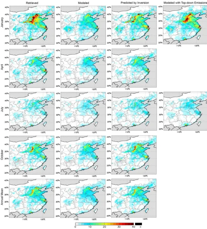
Figure 4 compares retrieved VCDs with simulated values (from all sources; Case 1 in Table 2) for January, April, July, October and annual average for 2006. Retrieved VCDs are large in regions with more advanced economic and industrial development and/or dense population, including the coastal and neighbor provinces from Beijing to Shanghai, the Pearl River Delta and the Sichuan Basin. Spike values are evident over major cities. In addition, retrieved VCDs vary across the months significantly, reaching maximum values in Jan-uary and minimum values in July.
GEOS-Chem captures fairly well the spatial distributions of retrieved VCDs in different seasons (Fig. 4). The R2 for spatial correlation between modeled and retrieved VCDs reaches 0.64 for January and 0.53 for July (Table 3). The smaller correlation in July is in part because the native horizontal resolution of the CTM (0.667◦long×0.5◦lat) is
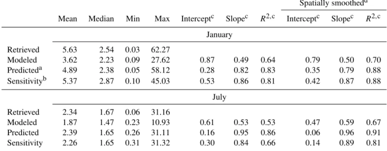
not fine enough to capture the large spatial variation of VCDs within short distances resulting from the short life-time of NOx (Martin et al., 2003; Lin et al., 2010a). Spa-tial smoothing of 5 gridboxes by 5 gridboxes (i.e. 1.25◦long by 1.25◦lat) results in a significant enhancement of model-retrieval correlation in July with theR2increasing to 0.67. The improvement ofR2due to the smoothing is moderate in January, compared to July, since the lifetime of NOxis longer and the spatial variability of VCDs within short distances is smaller and better simulated by GEOS-Chem.
GEOS-Chem underestimates the magnitude of retrieved VCDs particularly over polluted regions in wintertime (Fig. 4). The range of simulated VCDs is also narrower than the retrieved range: spatially, the modeled maximum VCD is lower than the retrieved maximum with the minimum being higher (Table 3). Averaged over East China, model VCDs are about 20 % lower than retrieved values in July and about 36 % lower in January (Table 3).
4 Inversion of anthropogenic, lightning and soil emissions
4.1 Method
As discussed in Sect. 3.1, anthropogenic emissions of NOx in East China exhibit weak seasonality and natural emissions reach maximum values in summer and minimum in winter (Fig. 2). In addition, the lifetime of NOxis shortest in sum-mer and longest in winter as a result of varying photochem-ical activity (Martin et al., 2003; Lin et al., 2010a; Lin and McElroy, 2010). This results in minimum values in summer for VCDs of NO2of anthropogenic origin and maximum val-ues for NO2 from natural sources, as simulated by GEOS-Chem (Fig. 5). Averaged over East China, natural sources contribute to about 30 % of the total abundance of NO2 in July and August, in contrast to their negligible contributions in winter months. This characteristic is exploited here to es-timate anthropogenic and natural emissions separately.
The inversion here involves a multi-step process based on a weighted multivariate linear regression analysis facilitated by several supplementary procedures. It is done gridbox by gridbox to derive the respective emissions. The regression is described in Sect. 4.1.1. The complete inversion process is described in Sect. 4.1.2 together with the supplementary procedures.
4.1.1 A weighted multivariate linear regression analysis for each gridbox
Neglecting horizontal transport and assuming a linear rela-tionship between the total VCD of NO2and VCDs from indi-vidual sources, the retrieved VCD of NO2for a given gridbox (of 0.25◦long×0.25◦lat) in a given month can be
approxi-mated as the sum of modeled VCDs from individual emission sources, multiplied by certain scaling factors, and a random error term:
Table 3.Statistics for retrieved and modeled VCDs of NO2in January and July 2006.
Spatially smoothedd
Mean Median Min Max Interceptc Slopec R2,c Interceptc Slopec R2,c
January
Retrieved 5.63 2.54 0.03 62.27
Modeled 3.62 2.23 0.09 27.62 0.87 0.49 0.64 0.79 0.50 0.70 Predicteda 4.89 2.38 0.05 58.12 0.28 0.82 0.83 0.35 0.79 0.88 Sensitivityb 5.37 2.87 0.10 45.03 0.53 0.86 0.81 0.42 0.87 0.88
July
Retrieved 2.34 1.67 0.06 31.16
Modeled 1.87 1.47 0.23 10.93 0.61 0.53 0.53 0.47 0.59 0.67 Predicted 2.39 1.65 0.26 31.11 0.16 0.95 0.86 0.06 0.96 0.91 Sensitivity 2.26 1.65 0.31 31.32 0.30 0.84 0.66 0.14 0.89 0.81
aPredicted from the regression-based inversion. bSensitivity simulation using the top-down emissions. cWith respect to retrieved VCDs.
dAfter 5 gridboxes by 5 gridboxes horizontal smoothing.
Hererdenotes retrieved VCD of NO2, andmdenotes modeled VCD. The error termεis assumed to follow a nor-mal distribution with zero mean and standard deviation (σ ) equal to the sum in quadrature of errors from r andm. The subscripts “a”, “l”, “s”, and “b” indicate anthropogenic, lightning, soil, and biomass burning sources of NOx, respec-tively. The VCD that can be predicted from the inversion process (p) is:
p=kam,a+klm,l+ksm,s+kbm,b (2) where eachkis an estimate of the correspondingKand is to be determined by the inverse modeling. The top-down emis-sion (Et) is calculated as the sum of the a priori emissions from individual sources multiplied by corresponding scaling factors:
Et=kaEa,a+klEa,l+ksEa,s+kbEa,b (3) Here a linear relationship is assumed for each source between emissions of NOx and VCDs of NO2. r, m andσ are known variables, and they vary from one month to the next. By minimizing the sum of [(r−p)/σ]2 in all months, Eqs. (1)–(2) serve as a weighted multivariate linear regres-sion model to determine the scaling factors. Here the scaling factors are assumed implicitly to be season independent.
Over China, the contribution of biomass burning is very small for NOx, thus we do not attempt to constrain the asso-ciated emissions: the respective scaling factor is set as unity. Emissions from lightning and soil vary with seasons with similar patterns (Fig. 2), thus it is difficult to distinguish their contributions accurately based on the regression approach. Therefore the scaling factors for the two sources are assumed
to be the same in conducting the regression analysis. Under these assumptions, Eqs. (1)–(3) reduce to:
r=Kam,a+Kl(m,l+m,s)+m,b+ε (4) p=kam,a+kl(m,l+m,s)+m,b (5) Et=kaEa,a+kl(Ea,l+Ea,s)+Ea,b (6) The regression model here provides a basic statistical tool to calculateka andkl. It is necessary to determine the ranges ofkaandklto facilitate the regression analysis; without such constraints the derived scaling factors may be unrealistic for certain gridboxes (too high, too low or even negative). kais set to range from 0.33 to 3 reflecting that uncertainties in an-thropogenic emissions are normally moderate for individual gridboxes. Uncertainties in natural emissions are expected to be larger than those in anthropogenic emissions, thereforekl is set to vary between 0.2 and 5. A larger range allowable for kl(e.g. 0.1–10) results in more extreme values ofklin several sparse locations with very low emissions, and has negligible impacts on the top-down emission budgets for East China.
4.1.2 A multi-step inversion process beyond the regression analysis
Fig. 3. (a)Seasonal variations of monthly mean near-surface (2 m) air temperature and precipitation observed from 284 meteorological stations over East China and modeled by GEOS-5. The observation data are taken from the global hourly dataset (DS3505) archived in the National Oceanic and Atmospheric Administration (NOAA) National Climatic Data Center (NCDC) (http://www7.ncdc.noaa. gov/CDO/cdo; see Lin et al., 2010b). Data from GEOS-5 are sam-pled at the meteorolgocal stations for consistency with the obser-vations. (b) Spatial distribution of the month-to-month correla-tion between a priori anthropogenic and natural (lightning + soil) emissions.
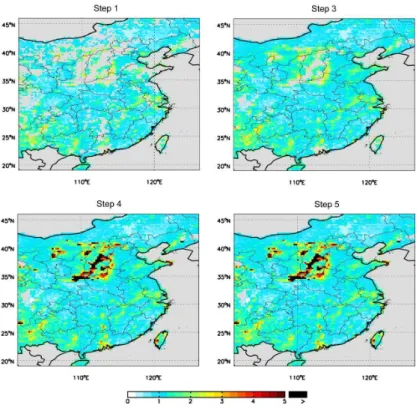
Gridboxes are assigned to group 1 if the ratior/mfor a selected winter month is smaller than the ratio for a selected summer month; otherwise they are assigned to group 2. For gridboxes in group 1, the regression analysis is performed to calculatekaandkl(step 1 in Fig. 6). Results are discarded if the regression is not statistically significant at a significance level of 0.1 under the Chi-square test. Spatial interpolation (step 2 in Fig. 6) is then conducted iteratively to deriveklfor all gridboxes: for a gridbox with undeterminedkl, the value
ofklis calculated as the geometric mean of values in the sur-rounding 24 gridboxes derived previously. For gridboxes in group 2, the regression analysis usually results in unrealisti-cally low values forkl and thus is used to estimateka only (step 3 in Fig. 6); the value ofklhas been determined at pre-vious steps. Again, the result is discarded if the regression is not statistically significant.
The regression approach may not be appropriate for cer-tain gridboxes with unrealistically larger/mratios in the winter month. This is because the scaling factorkalikely has a significant seasonal dependence as a result of the seasonal-ity in anthropogenic emissions not fully accounted for in the a priori dataset. These gridboxes are therefore reassigned to a third group, where akais derived for each month as the ratio [r−kl(m,l+m,s)−m,b]/ m,a(step 4 in Fig. 6). Ten-tatively, a gridbox is allocated to group 3 if the ratior/m exceeds 3, or if the ratio exceeds 2 withrbeing higher than 6×10¹⁵molec. cm−2, in the winter month.
As a final step, spatial interpolation is conducted to obtain kafor gridboxes of groups 1 and 2 where the regression is not statistically significant (step 5 in Fig. 6).
In group allocation and subsequent inversion process, each of three winter months (December, January and February) is paired with each of two summer months (July and August) to generate a suite of six cases for winter-summer contrast. (June is not selected since the contribution of natural sources to the total abundance of NO2is not as significant as that in July or August). Results from the six cases are combined to obtain final values of ka and kl. Specifically, results at a given step available from any or all of the six cases are geometrically averaged to obtain final values ofkaandkl, if and only if they have not been derived at earlier steps.
4.2 Scaling factors estimated for anthropogenic, lightning and soil sources
Fig. 5. Seasonal variations of VCDs of NO2(1015molec. cm−2)over East China for 2006 resulting from anthropogenic, lightning, soil
and total emissions of NOxmodeled by GEOS-Chem and predicted by the inversion. Also included is the seasonality of VCDs retrieved
from OMI.
Fig. 6. Description of the regression-based step-by-step inversion process after gridbox grouping. Values of kl are determined at
steps 1 and 2 for all gridboxes andka at steps 1, 3, 4, 5. See Sect. 4.1.2 for detailed analysis.
The special treatment at step 4 is taken mainly for grid-boxes in and around Shanxi Province and in parts of Ningxia and Inner-Mongolia (Fig. 7). These places are main areas in China for coal mining and coal-fired electricity generation. The large values ofka in these places, particularly in win-ter, suggest that the a priori dataset from INTEX-B likely underestimates anthropogenic sources related to use of coal, consistent with the findings of Wang et al. (2010).
The final values ofkaandklare determined at step 5 (see Fig. 7 for January) and step 2 (Fig. 8), respectively, for all gridboxes. They are used to calculate the top-down emis-sions for respective sources.
4.3 VCDs of NO2predicted from the inversion process
Compared to simulation results, predicted VCDs are much closer to retrieved values (Fig. 4). The spatial correlation between predicted and retrieved VCDs is much higher than the correlation between simulated and retrieved VCDs, with the R2 increasing from 64 % to 83 % in January and from 53 % to 86 % in July (Table 3). Averaged over East China, predicted VCDs are within 15 % of retrieved values across the seasons.
4.4 Top-down emissions
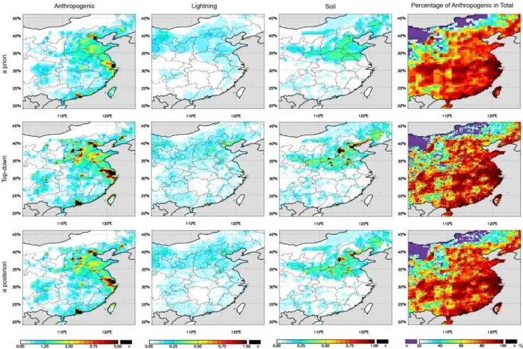
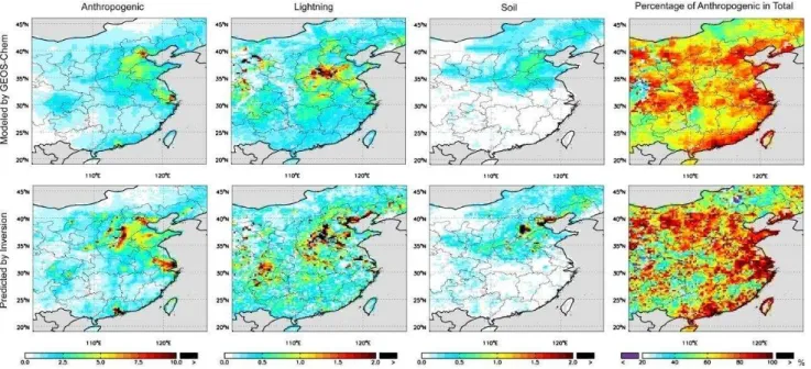
Figure 9 compares the top-down emissions of NOx for an-thropogenic, lightning and soil sources with respective a pri-ori emissions for July. Both top-down and a pripri-ori datasets suggest significant anthropogenic sources over the coastal provinces from Shanghai to Beijing and over the Pearl River Delta, resulting in large concentrations of NO2(Fig. 10). The top-down anthropogenic emissions are much higher than the a priori emissions in cities and at locations with extensive use of coal, especially in the northern provinces.
Fig. 7. Scaling factors for anthropogenic emissions (ka)determined at steps 1, 3, 4 and 5 of the inversion process described in Fig. 6 and
Sect. 4.1.2. Step 2 does not affectka and thus is not presented. Results at steps 4 and 5 are for January in particular. Areas outside the territory of China or with undeterminedkaare shown in grey.
Fig. 8.Scaling factors for lightning/soil emissions (kl) determined at steps 1 and 2 of the inversion process described in Fig. 6 and Sect. 4.1.2.
These two steps decideklfor all gridboxes. Areas outside the territory of China or with undeterminedklare shown in grey.
and Levy, 1995; Wang et al., 1998; Steinkamp and Lawrence, 2011). More detailed comparisons with Steinkamp and Lawrence (2011) and Hudman et al. (2012) are conducted in Sect. 5.1.2.
The contribution of anthropogenic sources to the total emissions of NOxin July is generally consistent between the a priori and top-down datasets (Fig. 9). The anthropogenic contribution exceeds 80 % over large areas of East China, but is lower than 60 % over most of the northwest and Inner-Mongolia. It differs from the anthropogenic contribution to
Fig. 9.The a priori, top-down and a posteriori estimates of anthropogenic, lightning and soil emissions of NOx(1015molec. cm−2h−1)and
the anthropogenic contributions (in percentage) to total emissions for July 2006 over East China. Areas outside the territory of China are shown in grey.
effect is evident particularly over the southwest. The in-verse modeling study by Lin et al. (2010a) showed that an assumed 100 % increase (0.57 TgN yr−1)in top-down light-ning emissions resulted in a 15 % reduction (0.86 TgN yr−1) in top-down anthropogenic emissions for July 2008 over East China; that is, any NO2molecule originating from lightning is 1.5 times as likely to be observed by OMI than a NO2 molecule of anthropogenic origin, consistent with the analy-sis here. In addition, data for simulated VCDs are sampled at the time of day of satellite overpass from days with valid retrieval data; while data for monthly emissions are averaged over all time of day in all days of the month. The differ-ent sampling methods and the day-to-day and diurnal vari-ations in natural emissions may introduce some differences between anthropogenic contributions to total emissions and to total VCDs. Another possible cause is the neglect of hori-zontal transport likely introducing uncertainties in source at-tribution for relatively clean regions, e.g. at many places of Inner-Mongolia.
Table 1 compares the a priori and top-down emission bud-gets over East China for individual sources. Annually, the inversion results in budgets of 8.016 TgN, 0.228 TgN and
0.424 TgN for anthropogenic, lightning and soil emissions, respectively. These values are about 39 %, 31 % and 31 % larger than the corresponding a priori estimates. The top-down datasets also suggest that both lightning and soil emis-sions are less than 6 % of anthropogenic emisemis-sions. For July, the top-down budgets for lightning and soil emissions are 0.0623 TgN and 0.0810 TgN, respectively, about 10 % and 13 % of anthropogenic emissions estimated at 0.646 TgN.
4.5 Improved GEOS-Chem simulations using the top-down emissions
Fig. 10. VCDs of NO2(1015molec. cm−2)in July 2006 over East China resulting from anthropogenic, lightning and soil emissions of NOxand the anthropogenic contributions (in percentage) to the total VCDs modeled by GEOS-Chem and predicted by the inversion. Areas
outside the territory of China or without valid retrievals are shown in grey.
distribution of retrieved VCDs in both months. TheR2 for spatial correlation reaches a high level of 81 % for January and 66 % for July (Table 3). The smaller correlation in July is due to the short lifetime of NOx such that the CTM (at 0.667◦long×0.5◦lat) is not able to simulate the large spa-tial variation of NO2 within short distances, as discussed in Sect. 3.2. After (5 gridboxes by 5 gridboxes) horizontal smoothing, theR2increases to 88 % for January and 81 % for July (Table 3). Averaged over East China, the magnitude of model VCD is about 10 % higher than the predicted value in January and about 5 % lower in July (Table 3), indicating a slight nonlinear relationship between emissions and VCDs through the impacts on other species (HOx, ozone, etc.) and consequently on the lifetime of NOxand its partitioning into NO and NO2.
4.6 Sensitivity of emission inversion to embedded assumptions
This section evaluates the effects on the top-down emissions of several important assumptions taken during the inversion process, particularly for assumptions on the seasonality of various emission sources. The results are summarized in Table 1.
This study only includes 30 out of the 60 pixels from each OMI scan with smaller sizes in order to better analyze the spatial distribution of nitrogen within short distances. The top-down emission budgets for individual sources are similar to results from a sensitivity calculation employing OMI data from all pixels (Case 2 in Table 1); the differences are larger for individual locations (not shown).
The inversion approach allocates individual gridboxes to three groups prior to the regression. The effect of group allo-cation was evaluated by two tests, one by re-allocating grid-boxes in group 2 to group 1 and the other by re-allocating gridboxes in both group 2 and group 3 to group 1. The tests suggested that the effect of group allocation is less than 15 % for top-down lightning/soil emission budgets for East China (Cases 3 and 4 in Table 1) with much larger impacts for indi-vidual locations (not shown).
The regression accounts for the seasonal dependence of retrieval errors. A sensitivity test assuming a time invari-ant relative error of 30 % resulted in decreases by less than 5 % in top-down lightning/soil emissions (Case 5 in Table 1). Therefore the inversion approach is not sensitive to the sea-sonality of retrieval errors assumed here.
Another test was taken to evaluate the effect of errors in the Yienger and Levy (1995) soil emissions used as our a priori estimate. Specifically, the updated emission data by Hudman et al. (2012) (see Sect. 5.1.2 for specifications) were used to adjust modeled VCDs from soil sources (m,s) prior to the inversion, by scaling the VCDs for individual gridboxes with the ratios of Hudman et al. (2012) over Yienger and Levy (1995) soil emissions. As such, the annual top-down lightning emissions were reduced by 11 % and soil emissions enhanced by 19 % (Case 7 in Table 1). This is because of dif-ferences in seasonality (timing and magnitude) between soil emissions estimated by Hudman et al. (2012) and by Yienger and Levy (1995). The impacts of emission seasonality are analyzed further below.
Jaegl´e et al. (2005), Wang et al. (2007) and Zhao and Wang (2009) assumed lightning emissions to be simulated well by the CTM with no attempt to constrain them inversely. Under the same assumption, a sensitivity analysis was con-ducted by keeping lightning emissions unchanged during the inversion process here. This resulted in a 52 % increase in the top-down soil emission budget on the annual basis and a 41 % increase for July (Case 8 in Table 1).
If soil emissions are held unchanged during the inversion process, the top-down lightning emissions will be increased by less than 6 % (Case 9 in Table 1).
The inversion relies on modeled seasonal variations of lightning and soil emissions for separation from anthro-pogenic emissions. Due to similarity in seasonality, light-ning and soil sources cannot be separated unambiguously for a given gridbox. A total of nine additional tests were per-formed to further analyze the sensitivity of inversion results to assumptions on the seasonality of lightning and soil emis-sions, including the timing and magnitude (Cases 10–18 in Table 1). To test the timing of the seasonality,m,landm,s were shifted arbitrarily forward or backward by one month, separately or in combination, prior to the inversion process (Cases 10–15 in Table 1). As a result, top-down lightning and soil emissions are affected by up to 14 % on the regional mean basis. Another three tests evaluate the magnitude of the seasonality, by loweringm,l andm,s, separately and in combination, by 20 % in spring (March, April, May) and fall (September, October, November) and 40 % in summer (June, July, August). These changes have significant impacts on top-down lightning and soil emissions: by reducingm,l andm,ssimultaneously, top-down lightning and soil emis-sions were enhanced by about 33–34 % in July.
Convection lifts pollutants in the boundary layer to the up-per troposphere affecting the vertical distributions of vari-ous species. The magnitude of convection is highly param-eterized in current climate models and CTMs and thus con-tains large uncertainties (Tost et al., 2010). The importance of model convection for simulated VCDs of NO2originates from the altitude dependences of the lifetime of NOx, the fraction of NO2in NOx, and the averaging kernel that is ap-plied to the vertical distribution of NO2 (when comparing
with satellite retrievals). Its net effect can be estimated roughly by comparing NO2originating from a given amount of lightning emissions (i.e. located mostly at high altitudes) and NO2from the same amount of anthropogenic emissions (i.e. located mostly in the boundary layer). As suggested by Lin et al. (2010a) and discussed in detail in Sect. 4.4, any NO2molecule originating from lightning is 1.5 times as likely to be observed by OMI than a NO2molecule of anthro-pogenic origin for July 2008 over East China. Thus, doubling the magnitude of model convection and consequent changes in vertical distribution of NO2will result in a net increase by 50 % in modeled convection-associated VCD of NO2(when the averaging kernel is taken into account). To evaluate the impact of potential errors in model convection, a sensitivity test enhanced by 50 % the magnitude of convection of an-thropogenic NO2in July and August 2006, by tentatively in-creasing by 25 % modeled concentrations of anthropogenic NO2 above 500 hPa (Case 19 in Table 1). This effectively increased modeled anthropogenic VCDs of NO2 over East China by about 7.5 % in both months. It consequently re-sulted in a slight reduction in top-down anthropogenic emis-sions with reductions by about 4–5 % in top-down lightning and soil emissions (Case 19 in Table 1).
Errors in top-down emissions attributable to the inversion procedure are calculated as the sum in quadrature of percent-age deviations of all inversion results (Cases 2–19) relative to the base estimate (Case 1), added in quadrature with errors resulting from the nonlinearity between emissions of NOx and VCDs of NO2 that are not accounted for in the sensi-tivity tests. The nonlinearity derived errors are taken to be about 10 % for East China as a whole, based on discussions in Sect. 4.5. Thus, errors in top-down emissions for East China attributed to the inversion procedure are estimated to be about 12 %, 59 % and 69 % for anthropogenic, lightning and soil sources, respectively (Table 1).
4.7 Total errors in the top-down emission budgets over East China
The inverse estimate here is subject to errors in retrievals, errors in model simulations, and errors in the inversion pro-cedures as estimated from the sensitivity analyses. The total error in top-down emission budget over East China is taken to be the sum in quadrature of the three errors, amounting to about 52 %, 77 % and 85 % for anthropogenic, lightning and soil sources, respectively (Table 1).
5 A posteriori emissions
The a posteriori emissions are estimated as the average of the a priori and top-down emissions weighted by the inverse-square of their respective errors (Martin et al., 2003). Errors in the a priori emissions are taken to be 60 % for an-thropogenic sources (Wang et al., 2007; Zhao and Wang, 2009) increasing to 100 % for lightning and soil sources ac-counting for the large range of current estimates (Boersma et al., 2005; Jaegl´e et al., 2005; Schumann and Huntrieser, 2007; Wang et al., 2007; Zhao and Wang, 2009; Lin et al., 2010a). Errors in the respective top-down emissions are taken to be 52 %, 77 % and 85 %, as derived in Sect. 4.7. Note that the error estimates here are conducted for total emissions in East China. Errors at individual locations may be much larger for both a priori and top-down datasets; the derivation however requires more detailed information that is not available currently. Therefore the error estimates for regional emission budgets are applied to individual loca-tions, as a simplified procedure, in deriving the a posteriori emissions.
The a posteriori emissions for 2006 over East China amount to 7.060 TgN (±39 %) for anthropogenic sources, to 0.208 TgN (±61 %) for lightning sources, and to 0.382 TgN (±65 %) for soil sources (Table 1). For July, the a posteriori budgets are 0.575 TgN (±39 %), 0.0580 TgN (±61 %), and 0.0733 TgN (±65 %), respectively. The temporal and spatial distributions of the a posteriori emissions are presented in Figs. 2 and 9 for comparison with the a priori and top-down emissions.
5.1 Comparison with previous estimates
That anthropogenic emissions inferred from space are larger than bottom-up inventories for China is consistent with re-sults from many previous studies (Jaegl´e et al., 2005; Wang et al., 2007; Zhang et al., 2007; Lin and McElroy, 2011). Our a posteriori budget for anthropogenic emissions over East China is similar to the value of 0.565 TgN for July 2007 es-timated by Zhao and Wang (2009). This study further pin-points, at a higher resolution, cities and areas with extensive use of coal to be the main regions where bottom-up inven-tories likely underestimate anthropogenic emissions. Eval-uation of lightning emissions is more difficult due to the large uncertainty in current research (Boersma et al., 2005; Schumann and Huntrieser, 2007) and the significant interan-nual variability of lightning occurrences on the regional scale (Schumann and Huntrieser, 2007). Our a posteriori emis-sions are within the range of previous estimates (Boersma et al., 2005; Schumann and Huntrieser, 2007; Stavrakou et al., 2008).
Soil emissions of NOxover China are of great interest con-cerning the extensive use of fertilizers. A detailed analysis is conducted as follows for our a posteriori estimate of soil emissions.
5.1.1 Comparison with previous satellite-derived soil emission estimates
Wang et al. (2007) suggested that soil emissions are about 0.85 TgN per year for 1997–2000 over East China, amount-ing to 23 % of anthropogenic emissions on the annual ba-sis and to as much as 43 % for summer months. In bet-ter agreement with our estimates for East China, Jaelg´e et al. (2005) found an annual budget of∼0.40 TgN for 2000, and Zhao and Wang (2009) suggested soil emissions to be about 0.0883 TgN for July 2007 (L. Jaegl´e, personal commu-nication, 2011; C. Zhao and Y. Wang, personal communica-tion, 2011). The differences are derived mainly from satellite products and methods to separate anthropogenic and natural sources of NOxemployed in individual studies.
5.1.2 Comparison with recent bottom-up estimates for soil emissions
Two new bottom-up estimates have been conducted for soil emissions by Steinkamp and Lawrence (2011) and Hud-man et al. (2012), improving upon the work of Yienger and Levy (1995) used as our a priori emissions. The new esti-mates employ information from more recent and complete field measurements to estimate emission factors. They use soil moisture rather than precipitation amount to separate dry and wet soil conditions. Hudman et al. (2012) also use soil moisture to calculate the duration and strength of the N-pulsing. The two new estimates include updated infor-mation on fertilizer use and vegetation map. For fertilizer use, Steinkamp and Lawrence (2011) account for its interan-nual variation based on the FAO statistics; while Hudman et al. (2012) use the latest available gridded dataset from Pot-ter et al. (2010) representative of the year 2000. The two studies assume about 1.0 % and 0.62 %, respectively, of ni-trogen in fertilizers to be emitted as NOx, for better com-parisons with the observation-based estimate by Stehfest and Bouwman (2006). Hudman et al. (2012) combine satellite measurements for the growing season of vegetation and at-tribute 75 % of fertilizer derived emissions to the first month of the growing season. They also consider deposited nitro-gen species as an additional fertilizer-like source of NOx. Steinkamp and Lawrence (2011) update the leaf area index (LAI) data for calculating the canopy reduction factor; while Hudman et al. (2012) assume no canopy reduction.
6 Conclusions
A regression-based multi-step inversion approach is pro-posed to estimate emissions of NOx from anthropogenic, lightning and soil sources for 2006 over East China on a 0.25◦long×0.25◦lat grid. It exploits information on VCDs of tropospheric NO2retrieved from the OMI instrument by KNMI (the DOMINO product version 2). The nested GEOS-Chem model for East Asia is used to interpret the impacts of individual sources on VCDs of NO2 to facilitate the inver-sion analysis. The inverinver-sion is conducted gridbox by box to derive the respective emissions. For any given grid-box, anthropogenic and natural sources are separated based on their different seasonality; and lightning and soil emis-sions are considered together due to their similarity in sea-sonality. Differences in spatial patterns between lightning and soil emissions are used implicitly for source separation to some extent.
The inversion starts by allocating the gridboxes to three groups based on analyses of the ratio of retrieved over mod-eled VCDs in winter and summer. A multivariate regres-sion analysis is used then to derive emisregres-sions from individ-ual sources for all months, taking advantage of the seasonal patterns of different sources determined by the CTM. Ancil-lary procedures are taken to supplement the regression anal-ysis for gridboxes in different groups. Assumptions made during the inversion process contribute to errors in the top-down emission budgets for East China by∼12 % for anthro-pogenic sources,∼59 % for lightning sources and∼69 % for soil sources. Sensitivity simulations of GEOS-Chem driven by the top-down emission data reproduce the spatial distri-bution of VCDs retrieved from OMI, with theR2for spatial correlation reaching 0.88 for January and 0.81 for July after (5 gridboxes by 5 gridboxes) horizontal smoothing.
The inversion results in an annual budget of 7.060 TgN (±39 %) for the a posteriori anthropogenic emissions of NOx over East China, about 23 % larger than the INTEX-B dataset (Zhang et al., 2009) used as our a priori emissions. On the 0.25◦long×0.25◦lat grid, it is evident that the excess is greater over cities and areas with extensive use of coal, particularly in the north in winter.
The a posteriori budgets are 0.208 TgN (±61 %) and 0.382 TgN (±65 %) for lightning and soil emissions, respec-tively, for 2006 over East China. Both values are about 18 % higher than the respective a priori estimates, but are each less than 6 % of the a posteriori anthropogenic emis-sions. Even for July, the a posteriori lightning and soil emissions are only about 10 % and 13 % of anthropogenic emissions, respectively. Our results for soil emissions are consistent with recent bottom-up estimates by Steinkamp and Lawrence (2011) and Hudman et al. (2012) and previ-ous inverse estimates by Jaegl´e et al. (2005), Stavrakou et al. (2008) and Zhao and Wang (2009). They are however about half of the inverse estimate by Wang et al. (2007) who
suggested soil emissions to be more than 40 % of anthro-pogenic emissions in summer of 1997–2000.
In concluding, anthropogenic emissions are found to be the dominant source of NOxover East China for 2006, even in summer when natural sources reach maximum values. The contribution of anthropogenic emissions most likely has in-creased in more recent years due to their rapid growth (Lin and McElroy, 2011). In the future, the anthropogenic con-tribution may continue to increase along with the rapid eco-nomic and industrial development, if emission control is not taken successfully. The importance of nitrogen control has been recognized by the Chinese government, resulting in control strategies targeting the power sector. However, the successfulness of nitrogen control also depends on changes in emissions from other sectors, particularly the industrial sector for which the current inventories may be subject to much larger uncertainties than for the power sector (Zhao et al., 2011). Further research is required to evaluate the ef-fectiveness of nitrogen control and resulting impacts on the contributions of anthropogenic versus natural sources to at-mospheric nitrogen burdens.
Acknowledgements. This research is supported by the National Natural Science Foundation of China, grant 41005078 and 41175127. We acknowledge the free use of tropospheric NO2
column data from www.temis.nl.
Edited by: A. Richter
References
Allen, D. J. and Pickering, K. E.: Evaluation of lightning flash rate parameterizations for use in a global chemical transport model, J. Geophys. Res., 107, 4711, doi:10.1029/2002jd002066, 2002. Boersma, K. F., Eskes, H. J., Meijer, E. W., and Kelder, H. M.:
Esti-mates of lightning NOxproduction from GOME satellite
obser-vations, Atmos. Chem. Phys., 5, 2311–2331, doi:10.5194/acp-5-2311-2005, 2005.
Boersma, K. F., Eskes, H. J., Veefkind, J. P., Brinksma, E. J., van der A, R. J., Sneep, M., van den Oord, G. H. J., Levelt, P. F., Stammes, P., Gleason, J. F., and Bucsela, E. J.: Near-real time retrieval of tropospheric NO2from OMI, Atmos. Chem. Phys.,
7, 2103–2118, doi:10.5194/acp-7-2103-2007, 2007.
Boersma, K. F., Eskes, H. J., Dirksen, R. J., van der A, R. J., Veefkind, J. P., Stammes, P., Huijnen, V., Kleipool, Q. L., Sneep, M., Claas, J., Leit˜ao, J., Richter, A., Zhou, Y., and Brunner, D.: An improved tropospheric NO2 column retrieval algorithm for
the Ozone Monitoring Instrument, Atmos. Meas. Tech., 4, 1905– 1928, doi:10.5194/amt-4-1905-2011, 2011.
Chen, D., Wang, Y., McElroy, M. B., He, K., Yantosca, R. M., and Le Sager, P.: Regional CO pollution and export in China simu-lated by the high-resolution nested-grid GEOS-Chem model, At-mos. Chem. Phys., 9, 3825–3839, doi:10.5194/acp-9-3825-2009, 2009.
2003,
http://www.atmos-chem-phys.net/3/1285/2003/.
Hudman, R. C., Jacob, D. J., Turquety, S., Leibensperger, E. M., Murray, L. T., Wu, S., Gilliland, A. B., Avery, M., Bertram, T. H., Brune, W., Cohen, R. C., Dibb, J. E., Flocke, F. M., Fried, A., Holloway, J., Neuman, J. A., Orville, R., Perring, A., Ren, X., Sachse, G. W., Singh, H. B., Swanson, A., and Wooldridge, P. J.: Surface and lightning sources of nitrogen oxides over the United States: Magnitudes, chemical evolution, and outflow, J. Geophys. Res., 112, D12S05, doi:10.1029/2006jd007912, 2007. Hudman, R. C., Moore, N. E., Martin, R. V., Russell, A. R., Mebust, A. K., Valin, L. C., and Cohen, R. C.: A mechanistic model of global soil nitric oxide emissions: implementation and space based-constraints, Atmos. Chem. Phys. Discuss., 12, 3555–3594, doi:10.5194/acpd-12-3555-2012, 2012.
Huntrieser, H., Schlager, H., H¨oller, H., Schumann, U., Betz, H. D., Boccippio, D., Brunner, D., Forster, C., and Stohl, A.: Light-ning produced NOxin tropical, subtropical and midlatitude
thun-derstorms: New insights from airborne and lightning observa-tions, Geophys. Res. Abstr., EGU2006-A-03286, EGU General Assembly 2006, Vienna, Austria, 2006.
Jaegl´e, L., Steinberger, L., Martin, R. V., and Chance, K.: Global partitioning of NOxsources using satellite observations: Relative
roles of fossil fuel combustion, biomass burning and soil emis-sions, Faraday Discuss., 130, 407–423, doi:10.1039/b502128f, 2005.
Lin, J.-T. and McElroy, M. B.: Impacts of boundary layer mixing on pollutant vertical profiles in the lower troposphere: Impli-cations to satellite remote sensing, Atmos. Environ., 44, 1726– 1739, doi:10.1016/j.atmosenv.2010.02.009, 2010.
Lin, J.-T. and McElroy, M. B.: Detection from space of a reduction in anthropogenic emissions of nitrogen oxides during the Chi-nese economic downturn, Atmos. Chem. Phys., 11, 8171–8188, doi:10.5194/acp-11-8171-2011, 2011.
Lin, J.-T., McElroy, M. B., and Boersma, K. F.: Constraint of anthropogenic NOxemissions in China from different sectors:
a new methodology using multiple satellite retrievals, Atmos. Chem. Phys., 10, 63–78, doi:10.5194/acp-10-63-2010, 2010a. Lin, J.-T., Nielsen, C. P., Zhao, Y., Lei, Y., Liu, Y., and
McEl-roy, M. B.: Recent Changes in Particulate Air Pollution over China Observed from Space and the Ground: Effectiveness of Emission Control, Environ. Sci. Technol., 44, 7771–7776, doi:10.1021/es101094t, 2010b.
Martin, R. V., Jacob, D. J., Chance, K., Kurosu, T. P., Palmer, P. I., and Evans, M. J.: Global inventory of nitrogen oxide emis-sions constrained by space-based observations of NO2columns,
J. Geophys. Res., 108, 4537, doi:10.1029/2003JD003453, 2003. Martin, R. V., Sioris, C. E., Chance, K., Ryerson, T. B., Bertram, T. H., Wooldridge, P. J., Cohen, R. C., Neuman, J. A., Swanson, A., and Flocke, F. M.: Evaluation of space-based constraints on global nitrogen oxide emissions with regional aircraft measure-ments over and downwind of eastern North America, J. Geophys. Res., 111, D15308, doi:10.1029/2005JD006680, 2006.
Moorthi, S. and Suarez, M. J.: Relaxed Arakawa-Schubert – A Pa-rameterization of moist convection for general-circulation mod-els, Mon. Weather Rev., 120, 978–1002, 1992.
M¨uller, J.-F. and Stavrakou, T.: Inversion of CO and NOxemissions
using the adjoint of the IMAGES model, Atmos. Chem. Phys., 5, 1157–1186, doi:10.5194/acp-5-1157-2005, 2005.
Murray, L. T., Jacob, D. J., Logan, J. A., and Koshak, W.: Improv-ing techniques for satellite-based constraints on the lightnImprov-ing pa-rameterization in a global chemical transport model, 11th Con-ference on Atmospheric Chemistry, January 14, 2009.
Murray, L. T., Jacob, D. J., and Logan, J. A.: Investigating lightning-driven interannual variability in the oxidative capac-ity of the troposphere, Geophys. Res. Abstr., EGU2010-14332, EGU General Assembly 2010, Vienna, Austria, 2010.
Murray, L. T., Logan, J. A., Jacob, D. J., and Hudman, R. C.: Spatial and interannual variability in lightning constrained by LIS/OTD satellite data for 1998–2006: implications for tropospheric ozone and OH, to be submitted to J. Geophys. Res., 2012.
Olson, J.: World Ecosystems (WEI.4): Digital raster data on a 10 minute geographic 1080×2160 grid, in Global ecosystems database, version 1.0: Disc A, NOAA Natl. Geophys, Data Cen-ter, Boulder, Colorado, 1992.
Ott, L. E., Pickering, K. E., Stenchikov, G. L., Allen, D. J., De-Caria, A. J., Ridley, B., Lin, R.-F., Lang, S., and Tao, W.-K.: Production of lightning NO(x) and its vertical distribution calculated from three-dimensional cloud-scale chemical trans-port model simulations, J. Geophys. Res.-Atmos., 115, D04301, doi:10.1029/2009jd011880, 2010.
Potter, P., Ramankutty, N., Bennett, E. M., and Donner, S. D.: Characterizing the Spatial Patterns of Global Fertilizer Ap-plication and Manure Production, Earth Interact., 14, 1–22, doi:10.1175/2009ei288.1, 2010.
Price, C., Penner, J., and Prather, M.: NOxfrom lightning, 1, Global
distribution based on lightning physics, J. Geophys. Res., 102, 5929–5941, doi:10.1029/96jd03504, 1997.
Richter, A., Burrows, J. P., N¨uß, H., Granier, C., and Niemeier, U.: Increase in tropospheric nitrogen dioxide over China observed from space, Nature, 437, 129–132, doi:10.1038/nature04092, 2005.
Rienecker, M. M., Suarez, M. J., Todling, R., Bacmeister, J., Takacs, L., Liu, H.-C., Gu, W., Sienkiewicz, M., Koster, R. D., Gelaro, R., Stajner, I., and Nielsen, E.: The GEOS-5 Data As-similation System – Documentation of Versions 5.0.1, 5.1.0, and 5.2.0, NASA, 2008.
Sauvage, B., Martin, R. V., van Donkelaar, A., Liu, X., Chance, K., Jaegl´e, L., Palmer, P. I., Wu, S., and Fu, T.-M.: Re-mote sensed and in situ constraints on processes affecting trop-ical tropospheric ozone, Atmos. Chem. Phys., 7, 815–838, doi:10.5194/acp-7-815-2007, 2007.
Schumann, U. and Huntrieser, H.: The global lightning-induced nitrogen oxides source, Atmos. Chem. Phys., 7, 3823–3907, doi:10.5194/acp-7-3823-2007, 2007.
Stavrakou, T., M¨uller, J. F., Boersma, K. F., De Smedt, I., and van der A, R. J.: Assessing the distribution and growth rates of NOx emission sources by inverting a 10-year record
of NO2 satellite columns, Geophys. Res. Lett., 35, L10801,
doi:10.1029/2008gl033521, 2008.
Stehfest, E. and Bouwman, L.: N(2)O and NO emission from agricultural fields and soils under natural vegetation: sum-marizing available measurement data and modeling of global annual emissions, Nutr. Cycl. Agroecosys., 74, 207–228, doi:10.1007/s10705-006-9000-7, 2006.
doi:10.5194/acp-11-6063-2011, 2011.
Streets, D. G., Bond, T. C., Carmichael, G. R., Fernandes, S. D., Fu, Q., He, D., Klimont, Z., Nelson, S. M., Tsai, N. Y., Wang, M. Q., Woo, J. H., and Yarber, K. F.: An inventory of gaseous and primary aerosol emissions in Asia in the year 2000, J. Geophys. Res.-Atmos., 108, 8809, doi:10.1029/2002jd003093, 2003. Tost, H., Lawrence, M. G., Br¨uhl, C., J¨ockel, P., The GABRIEL
Team, and The SCOUT-O3-DARWIN/ACTIVE Team: Uncer-tainties in atmospheric chemistry modelling due to convection parameterisations and subsequent scavenging, Atmos. Chem. Phys., 10, 1931–1951, doi:10.5194/acp-10-1931-2010, 2010. van der Werf, G. R., Randerson, J. T., Giglio, L., Collatz, G. J.,
Kasibhatla, P. S., and Arellano Jr., A. F.: Interannual variabil-ity in global biomass burning emissions from 1997 to 2004, At-mos. Chem. Phys., 6, 3423–3441, doi:10.5194/acp-6-3423-2006, 2006.
Wang, S. W., Streets, D. G., Zhang, Q. A., He, K. B., Chen, D., Kang, S. C., Lu, Z. F., and Wang, Y. X.: Satellite de-tection and model verification of NO(x) emissions from power plants in Northern China, Environ. Res. Lett., 5, 044007, doi:10.1088/1748-9326/5/4/044007, 2010.
Wang, S. W., Zhang, Q., Streets, D. G., He, K. B., Martin, R. V., Lamsal, L. N., Chen, D., Lei, Y., and Lu, Z.: Growth in NOx
emissions from power plants in China: bottom-up estimates and satellite observations, Atmos. Chem. Phys. Discuss., 12, 45–91, doi:10.5194/acpd-12-45-2012, 2012.
Wang, Y., Jacob, D. J., and Logan, J. A.: Global simulation of tropo-spheric O3-NOx-hydrocarbon chemistry 1. Model formulation,
J. Geophys. Res., 103, 10713–10726, 1998.
Wang, Y., McElroy, M. B., Martin, R. V., Streets, D. G., Zhang, Q., and Fu, T.-M.: Seasonal variability of NOxemissions over
east China constrained by satellite observations: Implications for combustion and microbial sources, J. Geophys. Res., 112, D06301, doi:10.1029/2006JD007538, 2007.
Yan, X. Y., Akimoto, H., and Ohara, T.: Estimation of nitrous ox-ide, nitric oxide and ammonia emissions from croplands in East, Southeast and South Asia, Glob. Change Biol., 9, 1080–1096, doi:10.1046/j.1365-2486.2003.00649.x, 2003.
Yan, X. Y., Ohara, T., and Akimoto, I.: Statistical modeling of global soil NO(x) emissions, Global Biogeochem. Cy., 19, GB3019, doi:10.1029/2004gb002276, 2005.
Yienger, J. J. and Levy, H.: Empirical model of global soil-biogenic NOxemissions, J. Geophys. Res., 100, 11447–11464, 1995.
Zhang, Q., Streets, D. G., He, K., Wang, Y., Richter, A., Bur-rows, J. P., Uno, I., Jang, C. J., Chen, D., Yao, Z., and Lei, Y.: NOxemission trends for China, 1995–2004: The view from the
ground and the view from space, J. Geophys. Res., 112, D22306, doi:10.1029/2007JD008684, 2007.
Zhang, Q., Streets, D. G., Carmichael, G. R., He, K. B., Huo, H., Kannari, A., Klimont, Z., Park, I. S., Reddy, S., Fu, J. S., Chen, D., Duan, L., Lei, Y., Wang, L. T., and Yao, Z. L.: Asian emis-sions in 2006 for the NASA INTEX-B mission, Atmos. Chem. Phys., 9, 5131–5153, doi:10.5194/acp-9-5131-2009, 2009. Zhao, C. and Wang, Y. H.: Assimilated inversion of NOxemissions
over east Asia using OMI NO2column measurements, Geophys.
Res. Lett., 36, L06805, doi:10.1029/2008gl037123, 2009. Zhao, Y., Nielsen, C. P., Lei, Y., McElroy, M. B., and Hao, J.: