<i>De praeceptis ferendis</i>: good practice in multi-model ensembles

(1)

ACPD

14, 15803–15865, 2014

De praeceptis ferendis

I. Kioutsioukis and S. Galmarini

Title Page

Abstract Introduction

Conclusions References

Tables Figures

◭ ◮

Back Close

Full Screen / Esc

Printer-friendly Version Interactive Discussion

Discussion

P

a

per

|

Discus

sion

P

a

per

|

Discussion

P

a

per

|

Discussion

P

a

per

Atmos. Chem. Phys. Discuss., 14, 15803–15865, 2014 www.atmos-chem-phys-discuss.net/14/15803/2014/ doi:10.5194/acpd-14-15803-2014

This discussion paper is/has been under review for the journal Atmospheric Chemistry and Physics (ACP). Please refer to the corresponding final paper in ACP if available.

De praeceptis ferendis

: good practice in

multi-model ensembles

I. Kioutsioukis1,2and S. Galmarini1

1

European Commission, Joint Research Center, Institute for Environment and Sustainability, Ispra (VA), Italy

2

Region of Central Macedonia, Thessaloniki, Greece

Received: 12 March 2014 – Accepted: 4 June 2014 – Published: 17 June 2014

Correspondence to: S. Galmarini (stefano.galmarini@jrc.ec.europa.eu)

(2)

ACPD

14, 15803–15865, 2014

Title Page

Tables Figures

◭ ◮

Back Close

Full Screen / Esc

Discussion

P

a

per

|

Discus

sion

P

a

per

|

Discussion

P

a

per

|

Discussion

P

a

per

|

Abstract

Ensembles of air quality models have been formally and empirically shown to outper-form single models in many cases. Evidence suggests that ensemble error is reduced when the members form a diverse and accurate ensemble. Diversity and accuracy are hence two factors that should be taken care of while designing ensembles in order

5

for them to provide better predictions. There exists a trade-oﬀ _{between diversity and}

accuracy for which one cannot be gained without expenses of the other. Theoretical aspects like the bias-variance-covariance decomposition and the accuracy-diversity decomposition are linked together and support the importance of creating ensemble that incorporates both the elements. Hence, the common practice of unconditional

av-10

eraging of models without prior manipulation limits the advantages of ensemble aver-aging. We demonstrate the importance of ensemble accuracy and diversity through an inter-comparison of ensemble products for which a sound mathematical framework ex-ists, and provide specific recommendations for model selection and weightingfor multi model ensembles. To this end we have devised statistical tools that can be used for

15

diagnostic evaluation of ensemble modelling products, complementing existing opera-tional methods.

1 Introduction

A forecast is considered complete if it is accompanied by an estimate of its uncer-tainty (AMS, 2002). This generally requires the embedding of the modelling process

20

into either a deterministic perturbation scheme (e.g., tangent linear, direct decoupled) or a probabilistic framework (e.g., Monte Carlo). Such approaches are used to quan-tify the eﬀ_{ects of uncertainties arising from variations in model input (e.g., initial and}

boundary conditions, emissions) or model structure (e.g., parameterizations, numeri-cal discretization).

(3)

ACPD

14, 15803–15865, 2014

Title Page

Tables Figures

◭ ◮

Back Close

Full Screen / Esc

Discussion

P

a

per

|

Discus

sion

P

a

per

|

Discussion

P

a

per

|

Discussion

P

a

per

Deterministic approaches are fast but they rely on the validity of the linearized ap-proximation of error growth (Errico, 1997). The availability of computing means in recent years has boosted the application of the probabilistic approach (Leith, 1974) because it can sample the sources of uncertainty and their eﬀ_{ect on the prediction error in}

a non-linear fashion without requiring model modifications. However, the sampling of

5

the whole range of uncertainty could be quantified with the construction of very large sets of simulations that correspond to alternative configurations (data or model). This is unrealistic for 3-D models and leads to a hybrid scheme calledensemble forecasting (Molteni et al., 1996; Tracton et al., 1993). It is probabilistic in nature but it generally does not sample the input uncertainty in a formal mathematical way, limiting the extent

10

of the available mathematical bibliography to interpret the results.

Single model ensembles (e.g. Mallet et al., 2006) assume the model is perfect and consist from a set of perturbed initial conditions and/or physics perturbations. It is tra-ditionally used in weather forecasting, which is primarily driven by the initial conditions uncertainty.Multi model ensembles(e.g., Galmarini et al., 2004) (MME) quantify

prin-15

cipally the model uncertainty as they are generally applied to the same exercise (i.e. input data). This approach is usually implemented in air pollution and climate modelling studies, where the uncertainty is predominantly process driven. The models in a MME should ideally have uncorrelated errors. Under such condition, the deterministic fore-cast generated from the MME mean is better than any single-model forefore-cast due to the

20

averaging out of the errors (Kalnay, 2003). Besides that, the MME spread quantifies the output uncertainty, providing an estimate of the forecast reliability.

The simulation error of the ensemble mean outperforms the one of the individual ensemble members only if the assumption that the models are i.i.d. (independent and identically distributed around the true state), is satisfied (Knutti et al., 2010). The i.i.d.

25

(4)

ACPD

14, 15803–15865, 2014

Title Page

Tables Figures

◭ ◮

Back Close

Full Screen / Esc

Discussion

P

a

per

|

Discus

sion

P

a

per

|

Discussion

P

a

per

|

Discussion

P

a

per

|

example the analysis of extremes risky. Extra eﬀ_{ort is required in order to obtain an}

improved deterministic forecast such as the MME mean for i.i.d. members. The opti-mal solution requires some training phase, during which the models are manipulated towards the construction of an ensemble with a symmetric distribution around the truth. This can be achieved through either a weighting scheme that keeps all members (e.g.,

5

Potempski and Galmarini, 2009) or with a reduced ensemble (Galmarini et al., 2013; Solazzo et al., 2013) that makes use of only aneffective number of models. Both ap-proaches result in the optimum distribution of the models in the respective workspace. Ensembles tend to yield better results when there is a significant diversity among the models. Many ensemble methods, therefore, seek to promote diversity among the

10

models they combine. However, a definite connection between diversity and accuracy is still lacking. An accurate ensemble does not necessarily consist of independent mod-els. There are conditions under which an ensemble with redundant members could be more accurate than one with independent members. Seen from another angle, similar to diversity, ensembles also tend to produce better results when they contain negatively

15

correlated models. Ideally, the most accurate ensemble consists of members that are identically distributed around the observations. This property could not be parameter-ized as a monotonic function of characteristic properties for the selected members like independence, redundancy, etc.

In this work, we demonstrate the properties of a MME through the unprecedented

20

database built from regional air quality models within the Air Quality Modelling Evalu-ation InternEvalu-ational Initiative (AQMEII). The idea is to exploit ways to promote the prop-erties, through model selection or weighting, that guarantee a symmetric distribution of errors. This will require a training phase and will lead to a comparison between static and dynamic weights and their temporal scales predictability. Our motivation is to depict

25

some best practices for air quality ensembles.

(5)

ACPD

14, 15803–15865, 2014

Title Page

Tables Figures

◭ ◮

Back Close

Full Screen / Esc

Discussion

P

a

per

|

Discus

sion

P

a

per

|

Discussion

P

a

per

|

Discussion

P

a

per

and their impact on the output error using the AQMEII data. In Sect. 5 we extent the results obtained in the previous section into spatial forecasting. Conclusions are drawn in Sect. 6.

2 Theoretical considerations

The aim of this section is to outline the documented mathematical evidence towards

5

the reduction of the ensemble error. The following notation is used throughout the text:

Ensemble members (output of modelling systems) fi

Ensemble f =

M X

i=1

wifi, X

wi =1

Desired value (measurement) µ

10

whereMis the number of available members andwi are the weights.

3 The bias-variance-covariance decomposition of the error

The bias-variance decomposition states thatthe squared error of a model can be bro-ken down into two components: bias and variance.

MSEf=_E

f −µ2

15

=_E

f −µ2

−hEf −µi2+h_E_f₋_µ

i2

(6)

ACPD

14, 15803–15865, 2014

I. Kioutsioukis and S. Galmarini Title Page Abstract Introduction Conclusions References Tables Figures ◭ ◮ ◭ ◮ Back Close

Full Screen / Esc

Printer-friendly Version Interactive Discussion Discussion P a per | Discus sion P a per | Discussion P a per | Discussion P a per |

The two components usually work in opposition: reducing the bias causes a variance enhancement, and vice versa. Thedilemmais thus finding an optimal balance between bias and variance in order to make the error as small as possible (Geman et al., 1992; Bishop, 1995).

The error decomposition of a single model (case M=_{1 in Eq. 1) can be extended}

5

to an ensemble of models, in which case the variance term becomes a matrix whose oﬀ_{-diagonal elements are the covariance among the models and the diagonal terms}

are the variance of each model:

Varhf −µi=_Var

1

M

X

f_i−µ

= 1

M2Var hX

(f_i−µ)i

= 1

M2 

 X

Var (f_i−µ)+₂X

i <j

Cov f_i−µ,f_j−µ   10 =1 M 1 M X

Var (fi−µ)

+M−1

M



 1 M(M−1)

2 X

i <j

Cov fi−µ,fj−µ





=1

MVarE+

1− 1

M

CovE

h

Biasf,µi2=

1

M

X

fi−µ 2 = 1 M X (fi−µ)

2

=_bias2

Thus,the squared error of ensemble can be broken into three terms, bias, variance 15

and covariance. Substituting the terms in Eq. (1), thebias-variance-covariance decom-position (Ueda and Nakano, 1996; Markowitz, 1952) is presented as follows:

MSEf=_bias2+ 1

MvarE+

1− 1

M

covE (2)

Equation (2) is valid for uniform ensembles, i.e.w_i = 1

M. The terms bias and varE are

20

(7)

ACPD

14, 15803–15865, 2014

Title Page

Tables Figures

◭ ◮

Back Close

Full Screen / Esc

Discussion

P

a

per

|

Discus

sion

P

a

per

|

Discussion

P

a

per

|

Discussion

P

a

per

minus observed time-series) respectively while the new term covE is the average co-variance between pairs of distinct ensemble members error. From Eq. (2) follows:

– The more ensemble members we have, the closer is Varhf −µito covE;

– bias2and varE are positive defined, but covE can be either positive or negative.

The error of an ensemble of models not only depends on the bias and variance of

5

the ensemble members, but also depends critically on the amount of correlation among the model’s errors, quantified in the covariance term. Thecovarianceterm indicates the diversityordisparity between the member networks as far as their error estimates are concerned. Hence, the more diverse the individual members an ensemble has, the less correlated they would be, which seems obvious. Given the positive nature of the

10

other two terms and the trade-oﬀ_{between them, the quadratic error is minimized only}

in cases the covariance term is as little as possible. The lower the covariance term, the less the error correlation amongst the models, which implies reduced error of the ensemble. This is the main reason whydiversity in ensembles is extremely important.

3.1 The accuracy-diversity decomposition of the error

15

Krogh and Vedelsby (1995) proved that at a single datapointthe quadratic error of the ensemble estimator is guaranteed to be less than or equal to the average quadratic error of the component models:

f −µ2=

M X

i=1

w_i(f_i−µ)2− M X

i=1

w_if_i−f2 (3)

20

(8)

ACPD

14, 15803–15865, 2014

I. Kioutsioukis and S. Galmarini Title Page Abstract Introduction Conclusions References Tables Figures ◭ ◮ ◭ ◮ Back Close

Full Screen / Esc

Printer-friendly Version Interactive Discussion Discussion P a per | Discus sion P a per | Discussion P a per | Discussion P a per |

ensemble, on a particular pattern. But, given that we have no criterion for identifying that best individual, all we could do is pick one at random. In other words, taking the combination of several models would be better on average over several patterns, than a method which selected one of the models at random.

The decomposition (3) is composed by two terms. The first is the weighted

aver-5

age error of the individuals (accuracy). The second is the diversity term, measuring the amount of variability among the ensemble member predictions. Since it is always positive, it is subtractive from the first term, meaning the ensemble is guaranteed lower error than the average individual error. The larger the diversity term, the larger is the ensemble error reduction. Here one may assume that the optimal error belongs to the

10

combination that minimizes the weighted average error and maximizes the variability among the ensemble members. However, as the variability of the individual members rise, the value of the first term also increases. This therefore shows that diversity itself is not enough; we need to get the right balance between diversity and individual accu-racy, in order to achieve lowest overall ensemble error (accuracy-diversity trade-oﬀ_).

15

Unlike the bias-variance-covariance decomposition, the accuracy-diversity decom-position is a property of an ensemble trained on a single dataset. The exact link be-tween the two decompositions is obtained by taking the expectation of the accuracy-diversity decomposition, assuming a uniform weighting. It can be proved that (Brown et al., 2005):

20

E 1 M

M X

i=1

(fi−µ)2− 1

M

M X

i=1

fi−f

2!

=_bias2+ 1

MvarE+

1− 1

M covE E 1 M M X

i=1

(fi−µ)2 !

= Ω +_bias2 ₍₄₎

E 1 M

M X

i=1

f_i−f2

!

= Ω₋1

MvarE−

1− 1

M

(9)

ACPD

14, 15803–15865, 2014

Title Page

Tables Figures

◭ ◮

Back Close

Full Screen / Esc

Discussion

P

a

per

|

Discus

sion

P

a

per

|

Discussion

P

a

per

|

Discussion

P

a

per

TheΩ_{term constitutes the interaction between the two parts of the ensemble error.}

This is the average variance of the models, plus a term measuring the average devia-tions of the individual expectadevia-tions from the ensemble expectation. When we combine the two sides by subtracting the diversity term from the accuracy term from the average MSE, the interaction terms cancel out, and we get the original bias-variance-covariance

5

decomposition back. The fact that the interaction exists illustrates why we cannot sim-ply maximize diversity without aﬀ_{ecting the other parts of the error – in e}ﬀ_{ect, this}

interaction quantifies the accuracy-diversity trade-oﬀ_{for uniform ensembles.}

3.2 The analytical optimization of the error

The two presented decompositions and their inter-connection are valid for uniform

en-10

sembles, i.e.wi =M1. Both indicate that error reduction in an ensemble can be achieved through selecting a subset of the members that have somedesired propertiesand tak-ing their arithmetic mean (equal weights). An alternative to this approach would be the use of non-uniform ensembles. Rather than selecting members, it keeps all models and the burden is passed to the assignment of thecorrect weights. A brief summary of

15

the properties of non-uniform ensembles is presented in the following paragraphs. The construction of the optimal ensemble has been exploited analytically by Potemp-ski and Galmarini (2009). They provide diﬀ_{erent weighting schemes for the case of}

uncorrelated and correlated models by means of minimizing the MSE. Under the as-sumed condition of the models independence of observations and assuming also that

20

the models are all unbiased (bias has been removed from the models through a sta-tistical post-processing procedure), the formulas for the one-dimensional case (single-point optimization) are given in Table 1. Also, whether correlated or not, the models are assumed as random variables (i.e. their distribution is identical).

The optimal weights correspond to the linear combination of models with the

min-25

(10)

ACPD

14, 15803–15865, 2014

Title Page

Tables Figures

◭ ◮

Back Close

Full Screen / Esc

Discussion

P

a

per

|

Discus

sion

P

a

per

|

Discussion

P

a

per

|

Discussion

P

a

per

|

of a 3-member ensemble, where models are uncorrelated, has lower MSE than the best candidate model only if the MSE ratio (worst/best) of the models is lower than 4. In other words, the RMSE ratio may not exceed 2, implying that the individual members should not be very diﬀ_{erent. The conditions for correlated models are more restrictive.}

Further, unlike the case of uncorrelated models, optimal weights for correlated models

5

can be negative (Table 1).

3.3 Weakness of the traditional practice

The material presented in this section demonstrated clearly through a well-defined mathematical formulation that building ensembles on the basis of “including as more models as possible to the pool and taking their arithmetic mean” is generally far from

10

optimal as it relies on conditions that are normally not fulfilled. At the same time, it provided the necessary ingredients for ensemble building, using either the entire mem-bers with weights assigned or a subset of them with equal weights. Specifically, the optimization of the ensemble error:

– through the bias-variance-covariance decomposition, points towards the bias

cor-15

rection of the models and the use of uncorrelated or negatively correlated ensem-ble members (equal weights, sub-ensemensem-ble);

– through the accuracy-diversity decomposition, relies on finding the trade-oﬀ_point

between accurate and diverse members (equal weights, sub-ensemble);

– through analytical formulas, provides weights for all ensemble members

de-20

pendent on their error covariances (Potempski and Galmarini, 2009) (unequal weights, full ensemble);

Unlike the simple arithmetic mean of the entire ensemble, it is clear that all aforemen-tioned cases require a learning process/algorithm. The aim of this work is to assess and compare the predictive skill of three ensemble products with well-defined

mathe-25

(11)

ACPD

14, 15803–15865, 2014

Title Page

Tables Figures

◭ ◮

Back Close

Full Screen / Esc

Discussion

P

a

per

|

Discus

sion

P

a

per

|

Discussion

P

a

per

|

Discussion

P

a

per

1. the arithmetic mean of the entire ensemble (mme)

2. the arithmetic mean of an ensemble subset (mme<), linked to the error decom-positions (2.1, 2.2)

3. the weighted mean of the entire ensemble (mmW), linked to the analytical opti-mization (2.3).

5

4 Example

In this section, we present a theoretical example aimed at illustrating the basic ingre-dients of ensemble modeling discussed. Fourteen samples of 5000 records each have been generated; thirteen corresponding to output of model simulations and one act-ing as the observations. These synthetic time-series have been produced with

Latin-10

hypercube sampling (McKay et al., 1979). The reason of selecting Latin-hypercube sampling over random sampling, besides the correct representation of variability across all percentiles (Helton and Davis; 2003), is its ability to generate random numbers with predefined correlation structure (Iman and Conover, 1982; Stein, 1987).

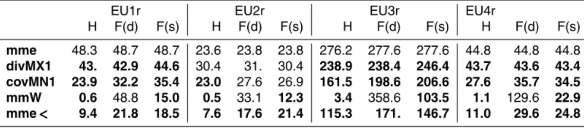
Figure 1 shows the RMSE distribution of the mean of all possible combinations of

15

the ensemble members (M=_{13) as a function of the ensemble size (}_k=_1,_{. . .}_,_M_{). The}

number of combinations of anyk members is given by the factorial M_k

, resulting in a total of 8191 combinations in this setting (e.g., 286 fork=_{3, 1716 for}_k=_{6, etc.). In}

the case of i.i.d. random variables (top row, left plot), increasing the number of members (k) moves the curves toward more skillful model combinations, as anticipated from the

20

bias-variance-covariance decomposition. Further, the optimal weights do not deviate from the equal weighting scheme (with small random fluctuations though) traditionally used in the MMEs. Hence, the optimal combination (mme<) and the optimal weighted combination (mmW) coincide. However the i.i.d. situation is unrealistic for MME, there-fore we will examine the ensemble skill by perturbing independently the three statistical

25

(12)

ACPD

14, 15803–15865, 2014

Title Page

Tables Figures

◭ ◮

Back Close

Full Screen / Esc

Discussion

P

a

per

|

Discus

sion

P

a

per

|

Discussion

P

a

per

|

Discussion

P

a

per

|

Bias has been introduced into the ensemble by shifting the distribution of two-third of the models by a small amount, making one-third of the models unbiased, one-third biased positively and one-third biased negatively. The RMSE distribution of all possible combinations (top row, right plot) does not appear symmetric with respect to the mean RMSE, with particular distortions at the maximum RMSE fork≤4 (i.e., one-third of

5

models). This upper bound is delineated from the ensemble combinations of all biased members of equal sign. Several combinations with multi-model error lower than the error of the full ensemble mean exist; at the same time, the whole RMSE distribution spans higher values compared to the i.i.d. case (note the change in scale). The optimal combination uses all unbiased models plus same amounts of biased equally members

10

from both sides. As for the weighted ensemble, no clue can be inferred as its weights by definition assume unbiased models.

The eﬀ_{ect of variance perturbations is displayed in the middle row. One third of}

the members (with ids 10–13 in particular) had deflated (left) or inflated (right) vari-ance. Due to the bias-variance dilemma, the case with smaller variance achieves lower

15

RMSE for lowk(at the expense of PCC though) while the opposite is true for the cases exhibiting larger variance. The optimal weighted combination gives higher weight to the under-dispersed members and lower weight to the over-dispersed ones.

All examined cases so far were uncorrelated. Next, a positive correlation (bottom row, left plot) has been introduced among the first three members (ids 1–3) and

sepa-20

rately, a negative correlation between two members (bottom row, right plot), with ids 5 and 8 namely. The upper (lower) bound of the error distribution of the combinations is distorted towards higher (lower) values by introducing positively (negatively) correlated members. Positively correlated members bring redundant information, where individual errors are added rather than cancelled out upon MME averaging. The optimal

combi-25

(13)

ACPD

14, 15803–15865, 2014

Title Page

Tables Figures

◭ ◮

Back Close

Full Screen / Esc

Discussion

P

a

per

|

Discus

sion

P

a

per

|

Discussion

P

a

per

|

Discussion

P

a

per

members are treated as one, negatively correlated are significantly promoted over the i.i.d. members.

To summarize, ensemble averaging is a good practice when models are i.i.d. In re-ality, models depart from this idealized situation and MME brings together information from biased, under- and over-dispersed as well as correlated members. Under these

5

circumstances, the equal weighting scheme or the use of all members well masks the benefits behind ensemble modelling. This example serves as a practical guideline to better understand the real issues faced when dealing with biased, inter-dependent members.

5 Empirical evidence

10

We now investigate the ensemble properties mentioned in the theoretical introduction using real-life spatially aggregated time-series from AQMEII (Rao et al., 2011). AQMEII was started in 2009 as a joint collaboration of the EU Joint Research Centre, the US-EPA and Environment Canada with the scope of bringing together the North American and European communities of regional scale air quality models. Within the initiative

15

the two-continent model evaluation exercise was organized which consisted in having the two communities to simulate the air quality over north America and Europe for the year 2006 (full detail in Galmarini et al., 2012a). Data of several natures were collected and model evaluated (Galmarini et al., 2012b). The community of the participating models, which forms a multi-model set in terms of meteorological driver, air quality

20

model, emission and chemical boundary conditions, is presented in detail in Galmarini et al. (2013). The model settings and input data are described in detail in Solazzo et al. (2012a, b), Schere et al. (2012), Pouliot et al. (2012), where references about model development and history are also provided.

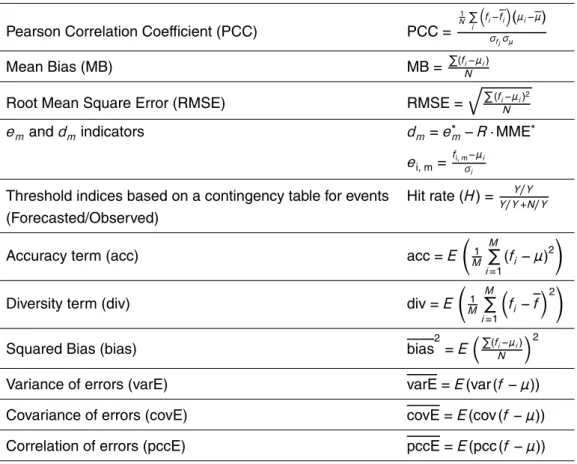
The analysis considershourly time-series for the JJA period. For European ozone,

25

the ensemble constitutes from thirteen models that give rise to 8191 diﬀ_erent

(14)

ACPD

14, 15803–15865, 2014

Title Page

Tables Figures

◭ ◮

Back Close

Full Screen / Esc

Discussion

P

a

per

|

Discus

sion

P

a

per

|

Discussion

P

a

per

|

Discussion

P

a

per

|

of the examined ensemble products (mme, mmW, mme<) will rely on several indices of error statistics. We present them in Table 2. Those metrics can be used for the val-idation of each single ensemble configuration (f_i) as well as for the ensemble mean (fens).

Once the basic ingredients have been identified, a spatial analysis will follow in the

5

next section.

5.1 Issue 1: properties of the MME error

According to the bias-variance-covariance decomposition, bias is an additive factor to the MSE and model outputs should be corrected for their bias before any ensemble treatment. The analytical optimization of the ensemble error and the defined weights

10

(Table 1) also assume bias corrected simulations. Here we do not intend to review the available algorithms for the statistical bias correction (e.g., Dosio and Paurolo, 2011); the correction applied in this work refers to a simple shift of the whole distribution without any scaling or multiplicative transfer function.

The RMSE of each possible combination as a function of the ensemble order

jus-15

tifies the statement obtained theoretically (Fig. 2, top left), namely that the RMSE of the ensemble mean is lower than the mean error of the single models. This does not prevent individual model errors to be lower than the ensemble mean error. The curve, although it originates from real data (EU4r), shares the same properties with its syn-thetic counterpart (previous section). Specifically:

20

– the ensemble average reduces themaximumRMSE as the order is increased

– a plateau is reached at the mean RMSE for k < M, indicating that there is no advantage, on average, to combine more thank members (k∼6).

– a minimum RMSE, among all combinations, systematically emerges for ensem-bles with a number of membersk < M (k∼3–6).

(15)

ACPD

14, 15803–15865, 2014

Title Page

Tables Figures

◭ ◮

Back Close

Full Screen / Esc

Discussion

P

a

per

|

Discus

sion

P

a

per

|

Discussion

P

a

per

|

Discussion

P

a

per

The probability density function (pdf) of the RMSE plotted fork=_{6 (similar for other}

values) demonstrates that there exist many combinations with lower error than the en-semble mean or the minimum of enen-semble mean and best single model. Those skilled groupings represent roughly 40 % of the total combinations in the first case, quasi con-stant across diﬀ_{erent sub-regions and below 40 % with high variability across di}ﬀ_erent

5

sub-regions (due to the spatial variability of best model’s skill) in the second case. This number is small (below 50 %) with non-random structure, implying that random draws from the pool of models is highly unlikely to produce better results than the ensemble mean; at the same time, it is high enough to leave space for significant improvements of the mme. The fractional contribution of individual models (fork=_{6) to those best}

10

sub-groups is given with the red numbers. The normalization has been done with the number of combinations that includes each model id (fork=_{6 it equals 792). For}

exam-ple, among all combinations, atk=_{6, that may contain the model with id 12, two-thirds}

of them (67 %) are skilful. The percentages indicate preference to combinations includ-ing more frequently some models (e.g., 4, 6, 9, 12) but at the same time they do not

15

isolate any single model. Further, the optimal weights of the full ensemble given with the bar plot (multiplied by a factor of 10) have a complex pattern as a result of diﬀ

er-ent model variances and covariances. Definitely, they depart from homogeneity (equal weighting scheme shown with the red straight line).

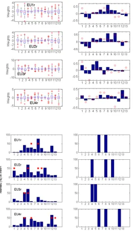
The error, variance and covariance (with observations) of the thirteen ensemble

20

members are presented in a Taylor plot (Fig. 2, top right). They visually form three clus-ters. Low skill cluster includes models 1, 2 and 10 that have the highest error, minimum correlation with observed data and appear under-dispersed. Model 5 also belongs to that group but has improved variance. The intermediate skill cluster contains models 3, 6, 7, 11 and 13 with average (11, 13) to low (3, 7, 6) error, correlation ranging from 0.8

25

(16)

ACPD

14, 15803–15865, 2014

Title Page

Tables Figures

◭ ◮

Back Close

Full Screen / Esc

Discussion

P

a

per

|

Discus

sion

P

a

per

|

Discussion

P

a

per

|

Discussion

P

a

per

|

belong to highest skill cluster; the contrary is true for the low skill cluster. Good mod-els have at least twice as much probability to form good ensemble groups compared to low skill models. On the other hand, even low skill models can yield good results under proper combination scheme. Overall, the multi-model average (mme) is a robust estimate with lower error than the candidate models but with reduced variance.

5

According to the presented decompositions, the combinations with reduced error should have a better balance between accuracy and diversity than the ensemble mean. A 2-dimensional plot of accuracy vs. diversity, with RMSE displayed as a third dimen-sion (in color) is shown in Fig. 2 (middle row, left). The black lines define the convex hull in the (accuracy, diversity) space of specific ensemble order, ranging from 2 in the

10

outer polygon to 12 (i.e. M-1) in the innermost one. As expected theoretically, the sep-arate optimization of accuracy and diversity will not produce the best ensemble output. For all ensemble orders, the optimal combination consists of accurate averaged repre-sentations of suﬃ_{cient diversity between members, i.e. with an ideal trade-o}ﬀ_between

accuracy and diversity. In particular, all skilled combinations are clearly seen in this

15

stratified chart; they form a well-defined area, traceable according to the ensemble or-der, that contains combinations with accuracy better than the average accuracy and ideal diversity (within a wide-range though) for the specific accuracy. For example, combinations of average accuracy form skilled ensemble products only if their diversity is very high. Analogously, combinations with very good accuracy form skilled ensemble

20

products only if their diversity is not relatively high. Diversity with respect to the ensem-ble mean can be derived independently to the observations. This however is not true for the accuracy part implying that a minimum training is required. Last, we observe that as ensemble order increases, accuracy and diversity become more and more bounded (with accuracy being more disperse than diversity), limiting any improvement. The

en-25

semble product with the right trade-oﬀ _{between accuracy and diversity (mme}_<_),

(17)

ACPD

14, 15803–15865, 2014

Title Page

Tables Figures

◭ ◮

Back Close

Full Screen / Esc

Discussion

P

a

per

|

Discus

sion

P

a

per

|

Discussion

P

a

per

|

Discussion

P

a

per

Similar results are obtained in terms of the variance-covariance decomposition in Fig. 2 (middle row, right). Here the convex hull areas, ranging from 3 to 12, move to-wards lower mean variance and higher mean covariance with increasing ensemble order. Higher spread is evidenced for the covariance term. As we include more mem-bers in the ensemble, the variance term in the decomposed error formula is becoming

5

lower but the covariance term is deteriorated. Skilful combinations have relatively low covariance. Ensembles consisting of highly correlated members bring redundant er-rors in the ensemble that does not cancel out upon averaging, producing overall bigger errors.

The conditions granting an ensemble superior to the best single model is also

at-10

tempted in Fig. 2 (last row). We have seen that the mme error is a function of accu-racy and diversity (or variance and covariance). An analytical optimization of this error (Potempski and Galmarini, 2009) yields the necessary conditions for being lower than the one of the best model (Table 1). For uncorrelated models, the only constrain is the skill diﬀ_{erence (MSE ratio) of the worst over the best single model; for correlated}

mod-15

els, it is more complex and it also related to the amount of redundancy in the ensemble, i.e. the error dependence. The explained variation by the highest eigenvalue reflects the degrees of freedom in the ensemble (and hence the redundancy). The pairwise plot as a function of the RMSE ratio of mme over the best single model (for ensemble or-der=_{6, left) shows that mme can outscore any single model provided the model error}

20

ratio and redundancy follows a specific pattern. For example, the benefits of ensemble averaging are devalued if we combine members that have big diﬀ_{erences in skill and}

dependent errors.

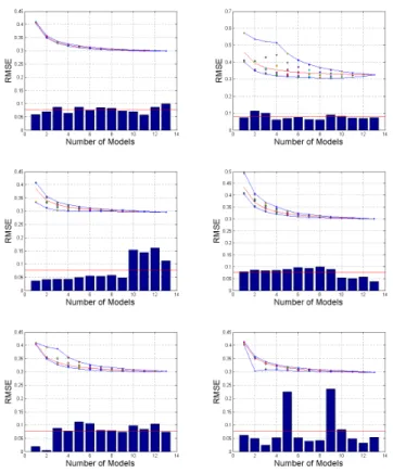
The distribution of the models around the truth should possess higher symmetry for the case of the skilled combinations. This thought is illustrated in Fig. 3 by means of

25

(18)

ACPD

14, 15803–15865, 2014

Title Page

Tables Figures

◭ ◮

Back Close

Full Screen / Esc

Discussion

P

a

per

|

Discus

sion

P

a

per

|

Discussion

P

a

per

|

Discussion

P

a

per

|

concentrations (over for min, under for max). The optimal combination (right plot) cor-responds to the models that are generally distributed randomly around the truth, i.e. when put together their errors cancel out upon averaging. This is evidenced across all percentiles. Such combinations are capable for studies ofextreme events. At the same time, their previsions have lower spread (i.e.uncertainty). As seen before, for the

se-5

lected ensemble order (k=_{3), the skilful combinations have small error covariance}

(they are both accurate and diverse).

To summarize, the unconditional averaging of ensemble members is highly unlikely to systematically generate a forecast with higher skill than its members across all per-centiles as models generally depart significantly from behaving as an i.i.d. sample.

Fur-10

ther, the ensemble mean is superior to the best single model given conditions that re-late to the individual skill of the members and the ensemble redundancy. Good practice includes bias correction of the models and the construction of a “balanced” ensemble through either a weighting approach (straightforward) or through the clustering of mem-bers with the desired properties (in the form of accuracy/diversity, variance/covariance,

15

redundancy, etc). In the next section we explore some measures to achieve such clus-ters.

5.2 Issue 2: clustering measures

Given a dataset ofN instances X=_{_X₁_,_X₂_,_{. . .}_,_X

N}, a clustering algorithm generates

r disjoint clusters based on a distance metric. Each clustering solution is a partition

20

of the dataset X into Ki (1≤i ≤r) disjoint clusters of instances. A typical output of a clustering algorithm is a dendrogram, where redundant models are grouped together and the level of similarity among groups is based on the distance between the ele-ments of the input matrix. Clustering algorithms are sensitive to the controlling options (theagglomerative method, thedistance metric, thenumber of clustersand thecut-off 25

(19)

ACPD

14, 15803–15865, 2014

Title Page

Tables Figures

◭ ◮

Back Close

Full Screen / Esc

Discussion

P

a

per

|

Discus

sion

P

a

per

|

Discussion

P

a

per

|

Discussion

P

a

per

utilized against two diﬀ_{erent input matrices, namely the corr (}_e

i,ej) and the corr (di,

dj) (for details see Solazzo et al., 2013). Common practice suggests cutting the den-drogram at the height where the distance from the next clustered groups is relatively large, and the retained number of clusters is small compared to the original number of models (Riccio et al., 2012). For this reason, thecut-offvalue(the threshold similarity

5

above which clusters are to be considered disjointed) is set to 0.10 for corr (d_i,d_j) and 0.4 for corr (e_i,e_j).

The application of the above produced five disjointed clusters (Fig. 4, top row). Look-ing at the corr (e_i,e_j) dendrogram (left plot) or the corr (d_i,d_j) dendrogram (right plot), for example, the two main branches at the top further split into two more at a relatively

10

low similarity level, suggesting a plausible way to proceed. A parallel inspection at the Taylor plot (Fig. 2) reveals the similarities of each cluster in terms of error, correlation and variance. Clustering according to corr (d_i,d_j) generates the visual clusters of the Taylor plor while corr (ei,ej) clustering is coarser. Many ensemble combinations with non-redundant members can be inferred from those plots; in addition, combinations

15

that should be avoided are also marked.

A decomposition of each deterministic model’s error into spectral components pro-vides another roadmap for clustering models. Using four components (ID, DU, SY, LT: for details see Galmarini et al., 2013) with the Kolmogorov–Zurbenco filter (Zurbenko, 1986), it is evident that the models with particularly high total error have all

deficien-20

cies with specific spectral component (Fig. 4, bottom row). The diurnal component in models 1, 2, 5 and 10 has error similar to the total error of the other models (from all components). If we repeat the analysis with two-component decomposition (ID+_DU,

SY+_{LT) that has limited energy leak between them, the conclusion still remains the}

same. Models with particular high systematic errors, as evidenced through the spectral

25

(20)

ACPD

14, 15803–15865, 2014

Title Page

Tables Figures

◭ ◮

Back Close

Full Screen / Esc

Discussion

P

a

per

|

Discus

sion

P

a

per

|

Discussion

P

a

per

|

Discussion

P

a

per

|

The integrated skill of the selected clusters through dendrograms or spectral analysis is compared through a Taylor plot (Fig. 4, bottom row). For all combinations, their trace is found in an area of high competence. At the same plot it is also displayed the skill of two products based on spectral optimization, namely the kzFO (1st order combination of the four optimal spectral components; see Galmarini et al., 2013) and kzHO (higher

5

order combination of two quasi-independent spectral components: ID+_{DU, SY}+_LT).

The kzFO provides a clear improvement over mme while the kzHO boosts further the mme<skill. The mean of those five independently generated products shows an im-provement over the mme (Fig. 2). Further, the spread of the formed ensemble products is lower compared to the deterministic model’s scatter, resulting in lower uncertainty.

10

Averaging ensemble products produced through an elegant mathematical approach that constrains their properties is a potential pathway to improvedforecastswith lower uncertainty. Last, we should point that no model was eventually excluded by the com-binations but all deterministic models have been utilized in at least one ensemble prod-uct.

15

To summarize, good practice includes the clustering of members through multiple diﬀ_{erent algorithms that operate on dissimilar properties (like redundancy, diversity,}

negative correlation, spectral decomposition, etc). Averaging those combinations gen-erated independently, hence having in principle uncorrelated errors, form a ground for skilled forecasts of lower uncertainty compared to the ensemble mean, increasing

fur-20

ther the forecast reliability.

5.3 Issue 3: ensemble training

In this section we will test the temporal and spatial robustness of our ensemble prod-ucts. We will work on the concepts of the least error combinations (mme<and mmW) using time series from diﬀ_{erent AQMEII sub-regions. Throughout this exploratory}

anal-25

(21)

ACPD

14, 15803–15865, 2014

Title Page

Tables Figures

◭ ◮

Back Close

Full Screen / Esc

Discussion

P

a

per

|

Discus

sion

P

a

per

|

Discussion

P

a

per

|

Discussion

P

a

per

The bias-variance-covariance decomposition requires negative correlation learning algorithms (e.g., Liu and Yao, 1999; Lin et al., 2008; Zanda et al., 2007); the accuracy-diversity decomposition relies on learning accuracy-diversity algorithms (e.g. Kuncheva, L. and Whitaker, 2003; Brown et al., 2005). The use of uncorrelated or diverse members alone, which are easily calculated through various metrics, does not imply an accurate

en-5

semble. For this reason, a global handy approach to optimal ensemble forecasting and member selection, based on proven mathematical statements, still does not ex-ist (ensemble output can be optimized through analytical formulas only for diagnostic problems). Therefore, the optimal approach under the current mathematical state is the ensemble training prior to forecasting, utilizing various approaches for model

weight-10

ing (e.g., Gneiting et al., 2005; Potempski and Galmarini, 2009) or sub-selecting (see Solazzo et al., 2013 for a presentation of reducing dimensionality approaches linked to redundancy). Some key elements of this process explored hereafter include the learning period, thealgorithmsand their controlling properties, theeffective number of modelsand theweight stability.

15

Learning period and scheme.The selection of the necessary training period should take into account the memory capacity of the atmosphere. Using complexity the-ory (e.g., Malamud and Turcotte, 1999), the ozone time-series demonstrates non-stationarity and strong persistence (e.g., Varotsos et al., 2012). This encourages the use of a scheme derived from an accurate recent representation of ozone to

medium-20

range forecasts (e.g. Galmarini et al., 2013).

Following the evidences presented in Sect. 4.1, bias-reduction should be always ap-plied prior to any ensemble manipulation. For this purpose, all simulations have been de-biased at each examined window size (e.g., 1 day, 3 months, etc). Results are shown for JJA 2006 at four selected sub-regions (AQMEII database), using variable

25

(22)

ACPD

14, 15803–15865, 2014

Title Page

Tables Figures

◭ ◮

Back Close

Full Screen / Esc

Discussion

P

a

per

|

Discus

sion

P

a

per

|

Discussion

P

a

per

|

Discussion

P

a

per

|

1. Error:The skill of the deterministic models, even after bias-correction, varies with location. A very good model at one site may perform averagely in another. As for the ensemble products:

– mme.The error of the ensemble mean is superior to the mean of the individ-ual model errors (proved analytically) but is not necessarily better than the

5

skill of the “locally” best model.

– mmW.The error of the weighted ensemble mean (mmW) is always superior since it has been analytically derived to minimize the MSE. For small window sizes (less than 4 days), the mmW error is superior to the theoretically derived ensemble error if models were uncorrelated (=_h_var_i_/_nm).

10

– mme<. The optimal error derived from a reduced-size ensemble mean (mme<) with the optimal accuracy-diversity trade-oﬀ _{is always lower than}

the error utilizing the full ensemble since models are not i.i.d. It is also, by construction, always lower than the best model’s error and higher than the mmW’s error.

15

2. Temporal sensitivity of the error:As the window size decreases, thehRMSEi de-crease due to the lowering of the error variance (bias correction is applied once in the 92 days case and 92 times in the daily cases). The relative amount of de-crease for mme is inversely proportional to the diurnal variability because bias correction has a more pronounced impact in cases with lower variance (Fig. 6).

20

For example, the largest (smallest) change is seen in EU2r (EU3r) that demon-strates the least (highest) variability. The cases with high variability, where the majority of models fail to simulate well, have a prominent improvement if treated with more sophisticated ensemble products such as the mmW and mme<. On the other hand, in cases where mme is better compared to the individual models,

25

(23)

ACPD

14, 15803–15865, 2014

Title Page

Tables Figures

◭ ◮

Back Close

Full Screen / Esc

Discussion

P

a

per

|

Discus

sion

P

a

per

|

Discussion

P

a

per

|

Discussion

P

a

per

3. mme vs. best model:In terms of the ensemble error gain, it is variable as it de-pends significantly on the individual model distributions around the truth. Without loss of generality, if we consider the 92 day case, we see that for all models the MSE ratio (worst/best) is lower than 4.37 (EU1r: 4.37, EU2r: 2.96, EU3r: 1.99, EU4r: 2.60). If models were uncorrelated, their mme would always be superior to

5

any single model since all ratios are smaller than 14 (=_M+_{1). Figure 5 shows}

that only in EU4r mme is better than the individual models. This occurs because for correlated models, the condition is also restricted by the redundancy (eigen-values spectrum). The RMSE ratio of mme over the best single model for the joint restrictions in the case of M (=_{13) correlated models (Fig. 2) shows that only}

10

in EU4r the explained variation by the highest eigenvalue has the correct value for the specified model MSE ratio [EU1r (67, 2.5), EU2r (64, 1.8), EU3r (76, 1.5), EU4r (59, 1.7)]. The isolines with RMSE ratio lower than one reflect the cases with a balanced distribution of members. Indeed, in EU4r (and EU2r), the distribution of the models around the observations is more symmetric, as can be seen in Fig. 6.

15

On the other hand, a significant departure from symmetry can be seen for EU1r and EU3r, resulting in a sub-optimal ranking of the mme. The distribution around the truth in the weighted ensemble (mmW) and the sub-ensemble (mme<) has always higher symmetry compared to mme, as can be seen in the same Figure.

4. mme vs. mme<: The estimation of the optimal weights is straightforward

(Ta-20

ble 1), but the sub-selection of members in mme< is not. Since mme< uses equal weights, we can apply the concepts deployed by the two error decomposi-tions and compare those properties with the ones of mme. We can then examine whether they can provide guidance towards members selection. Figure 7 displays the accuracy ratio (mme</mme) vs. the corresponding diversity ratio for all (92

25

(24)

ACPD

14, 15803–15865, 2014

Title Page

Tables Figures

◭ ◮

Back Close

Full Screen / Esc

Discussion

P

a

per

|

Discus

sion

P

a

per

|

Discussion

P

a

per

|

Discussion

P

a

per

|

– Improves mme<accuracy over mme and by a smaller portion lowers its di-versity (i.e. in big ensembles didi-versity is distorted less than accuracy). In other words, between accuracy and diversity, the controlling factor in those experiments in terms of error minimization is accuracy more than diversity. This is partially explained by the fact the accuracy values have higher spread

5

over diversity.

– Lowers mme<variance over mme (fewer members) and by a higher portion lowers its covariance. In other words, between variance and covariance, the controlling factor for error minimization is covariance more than variance.

Those findings indicate that, for example, focusing on learning diversity algorithms

10

(maximize diversity) does not guarantee an improvement over the mme whilst the min-imization of the model’s error covariance is more promising.

Effective number of models. Next we discuss the concept of the eﬀ_{ective number}

(Neﬀ) of models. In principle, Neﬀ reflects the degrees of freedom in the system (i.e.

number of non-redundant members that cover the output space ideally and hence, can

15

be used to generalize). It is not a property of the physical system (e.g. its principal modes of oscillation). An analytical way to calculateNeﬀ is through the formula

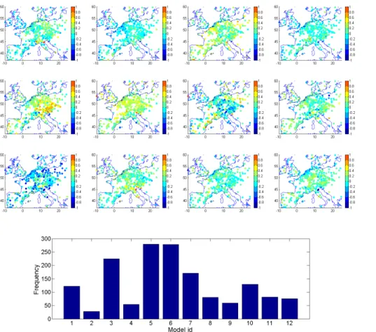
pro-posed by Bretherton et al. (1999). Using eigen-analysis, it estimates the number of models needed to reproduce the variability of the full ensemble (Fig. 8). Depending on the matrix whose skeleton is investigated (i.e. error, diversity, etc), diﬀ_{erent numbers}

20

arise forNeﬀ. For example, applying the eigen-analysis on the error matrix, regardless

if normalized or not, it yieldsN_eﬀ=3. IfNeﬀ is calculated using the diversity, it equals

5. The largest value (7) is obtained when Neﬀ is calculated using the dm matrix. Al-ternatively, one may calculate all possible combinations of models and plot them as a function of sub-ensemble size (as seen in Fig. 2). Comparing the range ofN_eﬀ found 25

through eigen-analysis (3–7) with the one found through error optimization (plateau of the minimum RMSE curve in Fig. 2), we observe that they coincide. In other words, the

Neﬀ calculated using thed_m (or diversity) matrix should provide the upper boundary of

(25)

ACPD

14, 15803–15865, 2014

Title Page

Tables Figures

◭ ◮

Back Close

Full Screen / Esc

Discussion

P

a

per

|

Discus

sion

P

a

per

|

Discussion

P

a

per

|

Discussion

P

a

per

Last, the fact that Neﬀ is generally less than the full ensemble size should not be

conceived that some models are useless. In fact, all models are likely to participate in the optimalNeﬀ combination, with diﬀerent frequencies though (Fig. 8). Unlike models,

as it has been demonstrated, many model combinations are useless.

Weight stability. We now explore the temporal robustness of the weighting schemes

5

in order to identify the predictive skill of the products. The spread of the weights (Fig. 9) is presented for two window sizes, 1 day (92 cases, left) and 92 days (1 case, right).

– The mmW weights arise from an analytical optimization approach and they are real numbers (i.e. can be negative). The significant error minimization seen ear-lier (Fig. 5) for the daily simulations originates from a highly variable weighting

10

scheme, lacking any autocorrelation pattern (not shown). The weights calculated over the whole JJA period (bar plot, right) do not generally have the same magni-tude with the mean weights of the daily blocks (red circle).

– The mme< weights arise from an exploratory optimization approach and they are binary numbers (0/1). The contribution (frequency) of each model in the daily

15

scheme (left panel), besides the peaks that vary by sub-region (a model is not optimal at all locations: for example, model 10 is frequently used in EU2r and never in EU4r), contain non-zero contribution from all ensemble members. Daily and seasonal contributions have more similarities than in the mmW case.

– Although calculated with diﬀ_{erent approaches, the weight peaks at seasonal scale}

20

(in absolute values) of the mmW and mme<are coherent.

Besides the day to day variability of the weights, we also explore another aspect of their temporal variability. The weights have been re-calculated for variable time-series length that is progressively increasing from 1 to 92 days, for the four European sub-regions (Fig. 10). Although no convergence actually occur, the mmW weights tend to

25

stabilize after 40–60 days. The same is approximately also true for the eﬀ_{ective number}

(26)

ACPD

14, 15803–15865, 2014

Title Page

Tables Figures

◭ ◮

Back Close

Full Screen / Esc

Discussion

P

a

per

|

Discus

sion

P

a

per

|

Discussion

P

a

per

|

Discussion

P

a

per

|

To summarize, the relative skill of the deterministic models radically varies with lo-cation. The error of the ensemble mean is not necessarily better than the skill of the “locally” best model, but its expectation over multiple locations is, making the ensem-ble mean a skilled product on average. A continuous spatial superiority over all single models is feasible in ensemble products such as mmW and mme<. As those products

5

require some training phase, good practice includes first, the identification of the tem-poral window length that allows robust (i.e. almost stationary) estimates for the weights and the eﬀ_{ective number of models (memory scale of the system) and then, the training}

of the ensemble at those temporal scales.

5.4 Issue 4: ensemble predictability

10

In the previous section we estimated weights for the full ensemble (mmW) or a subset of it (mme<) in a diagnostic mode. Following the explored temporal sensitivity of the weights and Neﬀ, in this section we examine the robustness of those estimates into

future cases. Are they capable of making accurate predictions or they just overfit the data over the historic epoch?

15

Two diﬀ_{erent sets of weights will be examined for each model, namely}_static_(weights

calculated over a 60 day window and applied on the remaining 30 daily forecasts) and dynamic(weights calculated over the most recent temporal window –day0– and applied on its successive –day0+_{1–). The reasoning behind the dynamic weighting testing is}

that, although weights (mmW) lack any autocorrelation pattern (i.e., what is optimal

20

yesterday is not optimal today), this does not imply that this quasi-optimal weighting for tomorrow is not still a good ensemble product (mmW weights are real, hence there are infinite weighting vectors where only one is optimal but there should exist many combinations without major skill diﬀ_{erence from the optimal).}

In view of the sensitivity of the dynamic weights vs. the static ones, we investigate the

25

(27)

ACPD

14, 15803–15865, 2014

Title Page

Tables Figures

◭ ◮

Back Close

Full Screen / Esc

Discussion

P

a

per

|

Discus

sion

P

a

per

|

Discussion

P

a

per

|

Discussion

P

a

per

(divMX1) or minimize error covariance (covMN1). The following conclusions can be inferred from Fig. 11 for the daily forecasts:

– Diversity alone generally does not outscore mme, neither with static nor with dy-namic weights. It gives similar results but can also produce worse forecasts when mme is well balanced between accuracy and diversity (EU2r). This experiment

5

shows that there may exist many diverse combinations of low accuracy. On the other hand, covariance (covMN1) is a more powerful indicator for ensemble opti-mization than diversity (divMX1).

– The weights derived through analytical optimization (mmW) do not correspond to products with similar properties between consecutive days. Dynamic weighting

10

can result at high MSE values for the prediction day. On the other hand, static weights outscore all other products.

– Mme<is always superior to the mme, in all examined modes (historic, prognostic with static/dynamic weights).

Weighting is a risky process (Weigel et al., 2010) and its robustness should be

thor-15

oughly explored prior to operational forecasting. In diagnostic mode (H), mmW min-imizes the error achieving an order of magnitude lower MSE compared to the other ensemble products (Table 3). In prognostic mode, the minimum error is obtained with mmW utilizing static weights, followed by mme<with static weights also. It is particu-larly noticeable the significant reduction of the peak MSE cases in those two schemes.

20

An improvement similar to the one obtained through the mmW scheme (bias correction, model weighting) has been documented in weather forecasting (Krishnamurti et al., 1999); the phenomenological diﬀ_{erent approaches in model weighting are however}

equivalent. Dynamic weights could be also used for the reduced ensembles, based ei-ther on diversity (divMX1), covariance (covMN1) or error (mme<) measures, but they

25