Understanding the critical distance in sparse distributed memory

(1)

marcelo salhab brogliato

(2)

(3)

Escola Brasileira de Administração Pública e de Empresas

-EBAPE

Fundação Getulio Vargas

U N D E R S TA N D I N G C R I T I C A L D I S TA N C E

I N S PA R S E D I S T R I B U T E D M E M O R Y

marcelo salhab brogliato

Computer Engineer. Instituto Militar de Engenharia,

2009

Dissertação submetida como requisito para a obtenção do

grau

Mestre em Gestão Empresarial

(4)

Ficha catalográfica elaborada pela Biblioteca Mario Henrique Simonsen/FGV

Brogliato, Marcelo Salhab

Understanding critical distance in sparse distributed memory / Marcelo Salhab Brogliato. – 2012.

126 f.

Dissertação (mestrado) - Escola Brasileira de Administração Pública e de Empresas, Centro de Formação Acadêmica e Pesquisa.

Orientador: Alexandre Linhares. Inclui bibliografia.

1. Memória - Simulação por computador. 2. Computadores neurais 3. Inteligência artificial distribuída. I. Linhares, Alexandre. II.

Escola Brasileira de Administração Pública e de Empresas. Centro de Formação Acadêmica e Pesquisa. III. Título.

(5)

banca examinadora:

Alexandre Linhares (Orientador - EBAPE-FGV) Flávio Codeço Coelho (EMAP/FGV)

Paulo Murilo Castro de Oliveira (IF-UFF)

Rafael Guilherme Burstein Goldszmidt (EBAPE-FGV)

local: Rio de Janeiro

data: Janeiro2012

Understanding Critical Distance in Sparse Distributed Memory ©

copyright byMarcelo Salhab Brogliato

2012

(6)

(7)

The love of a family is life’s greatest blessing.

— Author unknown

(8)

(9)

A B S T R A C T

Models of decision-making need to reflect human psychology. Towards this end, this work is based on Sparse Distributed Memory (SDM), a psychologically and neuroscientifically plausible model of human memory, published by Pentti Kanerva in 1988. Kanerva‘s model of memory holds a critical point: prior to this point, a previously stored item can be easily retrieved; but beyond this point an item cannot be retrieved. Kanerva has methodically calculated this point for a particu-lar set of (fixed) parameters. Here we extend this knowledge, through computational simulations, in which we analyzed this critical point behavior under several scenarios: in several dimensions, in number of stored items in memory, and in number of times the item has been rehearsed. We also derive a function that, when minimized, determines the value of critical distance according to the state of the memory. A secondary goal is to present the SDM in a simple and intuitive way in order that researchers of other areas can think how SDM can help them to understand and solve their problems.

R E S U M O

Modelos de tomada de decisão necessitam refletir os aspectos da psi-cologia humana. Com este objetivo, este trabalho é baseado na Sparse Distributed Memory (SDM), um modelo psicologicamente e neuro-cientificamente plausível da memória humana, publicado por Pentti Kanerva, em1988. O modelo de Kanerva possui um ponto crítico: um item de memória aquém deste ponto é rapidamente encontrado, e items além do ponto crítico não o são. Kanerva calculou este ponto para um caso especial com um seleto conjunto de parâmetros (fixos). Neste trabalho estendemos o conhecimento deste ponto crítico, através de simulações computacionais, e analisamos o comportamento desta

“Critical Distance”sob diferentes cenários: em diferentes dimensões; em

diferentes números de items armazenados na memória; e em diferentes números de armazenamento do item. Também é derivada uma função que, quando minimizada, determina o valor da“Critical Distance”de acordo com o estado da memória. Um objetivo secundário do trabalho é apresentar a SDM de forma simples e intuitiva para que pesquisadores de outras áreas possam imaginar como ela pode ajudá-los a entender e a resolver seus problemas.

(10)

(11)

Friendship is not something you learn in school. But if you haven’t learned the meaning of friendship, you really haven’t learned anything.

—Muhammad Ali

A C K N O W L E D G M E N T S

I must, first and foremost, give thanks for the complete and unwavering support and love from all my family. My wonderful parents Reynaldo and Angelina, my lovely sister Flávia, my sweet grandma Geny and all others who will always be remembered in my heart. Thank you for your patience and for understanding that I was physically far away but very close in heart. A special thanks to my dad, Reynaldo, who always taught me about life and who first awakened my passion for technology and engineering.

Thanks to Patricia Borges for sharing the dreams, the passion and the craziness, for all her caring and love; and for discussing about this work over and over again. Especially, for understanding my absence.

Three awesome guys taught me a lot about everything: comput-ing, psychology, anthropology, sociology, economics, and many others. Above all, I learned more about life. Thanks for every night of discus-sion filled with pizzas and diet coke, for the completely unexpected jokes and for believing in me. Thank you my good friends Alexandre Linhares, Claudio Abreu and Daniel Chada, in alphabetical order.

I feel really proud to be part of the Mestrado Acadêmico em Gestão Empresarial (MAGE) group. Formed by amazing people, always avail-able for serious talking, laughing and sharing their wide and deep knowledge, even at lunchtime and weekends. Special thanks to Ed-uardo Quintella, Isabel Silveira, Luiz Victorino, Sabrina Pavão and Sasha Nejain, in alphabetical order.

Thanks to professor Luiz Antônio Joia and Brigadier General Amir Elias Abdalla Kurban, who trusted me this task and made my mas-ter’s degree possible. Additionally, thanks to EBAPE / FGV for their excellent teachers and infrastructure.

Thanks to Instituto Militar de Engenharia for all the vast teachings that were absolutely essential to this work.

Finally, thanks to everyone who helped me in any way, for each word, for caring, for your support in difficult moments and for all jokes and talks that made my days worthwhile. Surely this work was done thanks to all of you. After all, nobody does it alone!

(12)

(13)

C O N T E N T S

i introduction 1

1 cognition, decision and administration 3 1.1 Cognitive Memory 5

ii sparse distributed memory 7 2 sparse distributed memory 9

2.1 Introduction 9

2.2 Neurons as pointers 13 2.3 Applications 13 2.4 Concepts 14 2.5 Read operation 14 2.6 Critical Distance 15

iii methodology 17 3 methodology 19 3.1 Simulations 19

3.2 Simulations environment 20 3.3 About the simulator 20

iv results 23

4 behavior of the critical distance on a sparse dis

-tributed memory 25 4.1 Introduction 25

4.1.1 Marks in figures 26

4.2 Influence of iterative-readings in Critical Distance 27 4.3 Influence of the number of writes in Critical Distance 27 4.4 Kanerva’s read vs Chada’s read 30

4.5 Unsuccessful attempt 30

4.6 Critical Distance through function minimization 35

v conclusions and future work 39 5 conclusions and future work 41

bibliography 43

Bibliography 43

vi appendix 47

a appendix a: first steps on simulator 49 a.1 Having some fun with Bitstrings 49

a.2 Simple writing and reading 50

b appendix b: additional iterative reading results for 1000-dimensional memory 53

c appendix c: additional iterative reading results for 256-dimensional memory 75

d appendix d: additional number of writings results for 256-dimensional memory 97

e appendix e: additional number of writings results for 1000-dimensional memory 103

(14)

L I S T O F F I G U R E S

Figure1 Activated addresses inside access radiusraround center address. 9

Figure2 Shared addresses between the target datumηand the cueηx. 10

Figure3 Hard-locations randomly sampled from binary space. 11

Figure4 In this example, four iterative readings were required to converge fromηx toη. 12

Figure5 Hard-locations pointing, approximately, to the target bitstring. 13

Figure6 Influence of number of iterative-readings in a1000-dimensional SDM memory 28

Figure7 Influence of number of iterative-readings in a256-dimensional SDM memory 29

Figure8 Influence of number of target writes in a1000-dimensional SDM memory 31

Figure9 Influence of number of target writes in a256-dimensional SDM memory 32

Figure10 Karnerva’s read compared to Chada’s read in a1000-dimensional SDM memory 33

Figure11 Karnerva’s read compared to Chada’s read in a256-dimensional SDM memory 34

Figure12 Unsuccessful attempt with value of adders to the power of three 35

Figure13 1000-dimensional, 1million hard-locations, 451

access radius,1write of target bitstring, Kanerva’s read,1iterative-reading 54

(15)

List of Figures xiii

(16)

xiv List of Figures

Figure53 256-dimensional,1million hard-locations,451 ac-cess radius,1write of target bitstring, Kanerva’s read,1iterative-reading 76

(17)

List of Figures xv

(18)

xvi List of Figures

(19)

Figure93 256-dimensional,1million hard-locations,451 ac-cess radius,1writes of target bitstring, Kanerva’s read,6iterative-reading 98

access radius,1 writes of target bitstring, Kan-erva’s read,6iterative-reading 104

(20)

L I S T O F TA B L E S

Table1 Write operation example in a7-dimensional mem-ory of dataηbeing written toξ, one of the acti-vated addresses. 13

Table2 Comparison of Kanerva’s read and Chada’s read. Eachξiis an activated hard-location and the val-ues come from their counters. Gray cells’ value is obtained randomly with probability50%. 15

A C R O N Y M S

KT Kemp-Tenenbaum

SDM Sparse Distributed Memory

AI Artificial Intelligence

GPU Graphics Processing Unit

GPGPU General Purpose Graphics Processing Unit

API Application Programming Interface

(21)

Part I

(22)

(23)

1

C O G N I T I O N , D E C I S I O N A N D A D M I N I S T R AT I O N

Which statement seems more true? (i) I have a brain. (ii) I am a brain.

— Douglas Hofstadter

One of the outstanding goals in the fields of administration, eco-nomics, and more generally, the applied social sciences, is to under-stand human behavior and decision-making. This work is based on the premise that the rational actor model is not psychologically plau-sible. The thriving results in fields such as decision-making, cognitive modeling and behavioral economics have shown a number of results corroborating this sweeping claim.

One of the tenets of management science is to develop a comprehen-sive theory of human decision-making. While the rational-decision actor has been successful in modeling and in bringing valuable insights into a number of decision scenarios, several studies have made clear that humans depart from rationality when faced with urgent, overwhelming or numerous choices (for recent summaries, see [30,7,8]).

Cognitive science, the study of human information-processing, is slowly filling the void between the need for formal models of human behavior and the numerous shortcomings of the rational model. The computational tools generated through the field’s explorations into human behavior can provide new paradigms of pattern recognition, exploratory data analysis and information retrieval, all central to the aim of decision science.

Take for example the field of business strategy: Gavetti[12,11] postu-lates that choice in novel environments, at least, is guided by analogy-making. Strategists and entrepreneurs perceive market opportunities in unfamiliar environments through analogies with better known firms, experiences and cases. (Case studies are, in fact, a highly popular tool in business education and their value often hinges on the understanding of one situation in terms of another.) Their work provides a number of examples of analogical reasoning:

i) The chain “Toys ‘R’ Us”, launched in the 1950s, was tied to the vision and success of supermarkets (the chain was effectively called “Baby Furniture and Toy Supermarket” at a particular point). After-wards, the launch of the office store “Staples” was based on similar reasoning: “Could we create a Toys R Us for office supplies?” [12];

ii) In the 1980s the largest European carmaker decided to invest heavily in the U.S. market by introducing a wide range of cars that were bestsellers in Europe. Before this decision, the carmaker had63% of the imported car market in the U.S. But the carmaker was called Volkswagen. The American consumer’s experience with Volkswagen consisted of the Beetle, an inexpensive and odd-looking car first sold in 1938. American consumers rejected the idea of a large, well-built, modern-looking, powerful and expensive Volkswagen. To make matters

(24)

4 cognition, decision and administration

worse, the company decided to withdraw the Beetle from the market, and its share of the imported car market in the U.S. dramatically fell from63% to less than4%. The exact same cars were being sold in Europe and in the U.S; the only difference was in the consumers’ experiences of what a “Volkswagen” meant. A twenty-thousand-dollar Volkswagen seemed, to Americans, like a practical joke. Similarly, “the new Honda” to an American consumer meant a new car model; to the Japanese, it meant a new motorcycle [29].

iii) When Iranian Ayatollah Ruhollah Khomeini declared afatwa(a death sentence) to writer Salman Rushdie, the Catholic Church did not stand for the principle of “Thou shalt not kill”. It recognized its experience of trying to censor the controversial film “The last temptation of Christ” and sided with the Iranians. L’Osservatore Romano, a key Vatican publication, condemned Rushdie’s book as “blasphemous”. The Head of the French Congregation, Cardinal Decourtray, called it an “insult to God”; Cardinal O’Connor from New York made it clear that it was crucial to “let Moslems know we disapprove of attacks on their religion” [15,21].

Decision-makers often obtain strategic insights by understanding one situation in terms of another; however, analogies are but one of the ideas from cognitive science that have crossed the bridge to manage-ment science. Neural Networks, or mathematical models of large-scale parallel processing in general, have found use in a number of more traditional management science applications, such as credit-risk evalua-tion [27], understanding new product development [26], and consumer targeting [20], to name a few.

The overwhelming majority of mathematical models of decision-making assume rationality. This often means an actor faces a set of actionsA={a1,a2,. . .,a3}. A consequence function maps each choice to a consequence:M:A_!C, and an utility functionU:C_!R_maps, finally, each consequence to the desirability of the outcome. The actor always chooses the actionak2Athat maximizes his utility function. A large number of authors have argued against this view, and there is ample body of evidence proving that the rational actor model, though practical for abstract models and manipulations, is unrealistic.

A key problem involved in these models is the lack of relevance. All actions must be considered by perfectly rational agents in order to maximize utility, or to guarantee that it is indeed maximized. In other words, there are no irrelevant acts; there are no acts that have been (or could have been) forgotten; there are no blind spots; there are no actions in the hypothetic space of possible actions that are left unconsidered. A potential act may be discarded, if its outcome is unwelcome, but it still must be considered.

A more realistic model of decision-making won’t take all these actions into account, but will, instead, consider the context in which decisions are and have been made and the past experiences encountered in similar situations. Many times, we realize that a better decision could have been made just after a sub-optimal decision has been taken. Sometimes we are able to realize this better option after a long while when a similar situation happens. This takes processing, and information-processing is limited.

(25)

1.1 cognitive memory 5

When one has insufficient past experience, one often makes analogies with situations with which we have more experience. Hofstadter argues that the core of learning and thinking is based on analogies[16,15]. Analogies are closely related to how our brain represents, processes and transforms information—main goals of cognitive science.

One can say that Artificial Intelligence (AI) researchers are also study-ing how to represent, process and transform information. Hofstadter[15] and Hawkins[13] don’t believe the AI field, as it is traditionally por-trayed, could answer these questions.

Traditional AI is based on optimizing search in the entire solution space. Of course this research field has yielded impressive results, such as solving mathematical theorems, playing chess, optimizing chain supply, routing from airplanes to electronic circuits, among other achievements. But in all these cases, the AI programs were only good at the one particular subject for which they were specifically designed. They can’t generalize or be flexible, and even their creators admit they don’t “think” like humans[13]. Our brain doesn’t work by searching and trying all possible choices. Furthermore, most of these programs could never handle imprecise inputs. For example, if you give them a problem similar to one it just solved, it needs to start its search of the hypothesis space all over again. Brains handle imprecision cues all the time. No situation presents itself exactly like a previous one. If you meet an old friend he will surely look at least a little different from the last time you met. This is not to say that search algorithms are not useful, on the contrary, they have and will always have important applications solving problems that are difficult for our brain to solve. But they are unable to solve the problems that the human brain could solve very easily.

1.1 cognitive memory

To explore and model the way in which our brain stores and retrieves our experiences is one of the main goals of cognitive memory research. This specific area of exploration tends to build models which exhibit the same properties that allow our memory to store and retrieve infor-mation from imprecise clues.

In his book, named On Intelligence[13], Jeff Hawkins says our brain could store the past and predict the future using imprecise clues from today. In other words, the human brain is always trying to predict what will happen based on the past, and we are constantly surprised when this prediction fails. Hawkins’ book is based on his studies of neocortex, the part of the brain that is involved in sensory perception, spatial reasoning, conscious thought and language. He also states that our neocortex isn’t a computer at all, but a memory system. Put another way, the thinking and the memory retrieving are intertwined, like the same thing. Hawkins argues that AI computes the solutions and there is a huge difference between computing a solution to a problem and using memory to solve the same problem.

(26)

6 cognition, decision and administration

store, retrieve and process information will mark a major breakthrough in science and technology.

(27)

Part II

(28)

(29)

2

S PA R S E D I S T R I B U T E D M E M O R Y

Everything in the plane of reality has been a dream one day.

— Leonardo Da Vinci

2.1 introduction

Sparse Distributed Memory (SDM) is a mathematical model for cog-nitive memory published by Pentti Kanerva in1988[19]. It introduces many interesting mathematical properties of n-dimensional binary space that, in a memory model, are psychologically plausible. Most notable among these are the tip-of-the-tongue phenomenon, conformity to Miller’s magic number (Linhares et al. 2011[22]) and robustness against loss of neurons.

Unlike traditional memory used by computers, SDM performs read and write operations in a multitude of addresses, also called neurons. That is, the data is not written, or it is not read in a single address spot, but in many addresses. These are called activated addresses, or activated neurons.

The activation of addresses takes place according to their distances from the datum. Suppose one is writing datum ηat addressξ, then all addresses inside a circle with center ξand radiusrare activated. So,ηwill be stored in all these activated addresses, which are around addressξ, such as in Figure1. An addressξ0_{is inside the circle if its} hamming distance to the centerξis less than or equal to the radiusr, i.e.distance(ξ,ξ0₎₆_r_.

η

Figure1: Activated addresses inside access radiusraround center address.

The data and address space belong to binary space and are repre-sented by a sequence of bits, called bitstrings. The distance between two bitstrings is calculated using the Hamming distance. It is defined for two bitstrings of equal length as the number of positions at which the bits are different. For example,00110b and01100b are bitstrings of length 5and their Hamming distance is2. One has to be careful when thinking intuitively about distance in SDM because the Hamming

(30)

10 sparse distributed memory

distance does not have the same properties that Euclidean distance does.

Every time you are writing or reading in SDM memory, a number of addresses are activated according to their distance to the center address and your data is written in these activated addresses or read from them. These issues will be addressed in due detail further on, but a major difference from a traditional computer memory is that your data are always stored and retrieved in a multitude of addresses. This way SDM memory has robustness against loss of addresses.

In traditional memory each datum is stored in an address and every time you are looking for a specific datum you have to search through the memory to find out whether you have it. In spite of computer scientists having developed many algorithms to perform fast searches, almost all of them do a precise search. That is, if you have an imprecise clue of what you need, these algorithms will simply fail.

In SDM, the data space is the same as the address space, which amounts to a vectorial, binary space, that is, a{0,1}n

space. This way, the addresses where the data will be written are the same as the data themselves. For example, the datumη=00101b 2{0,1}5will be written to the addressξ=η=00101b. If one chooses a radius of1, the SDM will activate all addresses one bit away or less from the center address. So, the datum00101bwill be written to the addresses00101b,10101b,

01101b,00001b,00111b and00100b. In this case, when one needs to retrieve the data, one could have an imprecise cue at most one bit away fromη, since all addresses one bit away haveηstored in themselves. Extending this train of thought for larger dimensions and radius, much more addresses are activated and one can see why SDM is a distributed memory.

When reading a cue ηx that is x bits away of η, the cue shares many addresses withη. The number of shared addresses decreases as the cue’s distance toηincreases, in other words, asxincreases. This is shown in Figure 2. The target datum η was written in all shared addresses, thus they will bias the read output in the direction ofη. If the cue is sufficiently near the target datumη, the read output will be closer toηthanηxwas. Repeating the read operation increasingly gets results closer toη, until it is exactly the same. So, it may be necessary to perform more than one read operation in order to converge to the target dataη.

η ηx

(31)

2.1 introduction 11

The addresses of the{0,1}n

space grows exponentially with the num-ber of dimensionsn, i.e.N=2n. Forn=100we haveN_⇡1030, which is incredibly big when related to a computer memory. Furthermore, Kanerva[19] suggestsnbetween100and10,000. Recently he has postu-lated10,000as a desirable minimumN(personal communication). To solve the feasibility problem of implementing this memory, Kanerva made a random sample of{0,1}n

, in his work, havingN0_{elements. All} these addresses in the sample are called hard-locations. Other elements of{0,1}n, not inN0_{, are called virtual neurons. This is represented in} Figure3. All properties of read and write operations presented before remain valid, but limited to hard-locations. Kanerva suggests taking a sample of about one million hard-locations.

Using this sample of binary space, our data space does not exist completely. That is, the binary space has2naddresses, but the mem-ory is far away from having these addresses available. In fact, only a fraction of this vectorial space is actually instantiated. Following Kanerva’s suggestion of one million hard-locations, forn=100, only

100_·106

/2100

= 7_·10−23 percent of the whole space exists, and for

n=1,000only100_·106

/21000

=7_·10−294_percent.

Kanerva also suggests the selection of a radius that will activate, on average, one one thousandth of the sample, which is 1,000 hard-locations for a sample of one million addresses. In order to achieve his suggestion, a1,000-dimension memory uses an access radiusr=451, and a256-dimensional memory,r=103.

N={0,1}n

N0 ξ1 ξ2 ξ3 virtual neurons hard-locations

Figure3: Hard-locations randomly sampled from binary space.

(32)

greater distances diverge. In Figure4, the circle has radius equal to the critical distance and every ηx inside the circle should converge. The figure also shows a convergence in four readings.

η

ηx ηx,1

ηx,2

ηx,3 critical distance

Figure4: In this example, four iterative readings were required to converge fromηxtoη.

The{0,1}n

space hasN = 2n locations from which we instantiate

N0_{samples. Each location in our sample is called a hard-location. On} these hard-locations we do operations of read and write. One of the insights of SDM is exactly the way we read and write: using data as addresses in a distributed fashion. Each datumηis written in every activated hard-location inside the access radius centered on the address, that equals datum,ξ=η. Kanerva suggested using an access radiusr

having about one one thousandth ofN0_{. As an imprecise cue}_η_x_shares hard-locations with the target bitstring η, it is possible to retrieveη

correctly. (Actually, probably more than one read is necessary to retrieve exactlyη.). Moreover, if some neurons are lost, only a fraction of the datum is lost and it is possible that the memory can still retrieve the right datum.

A random bitstring is generated with equal probability of0’s and

1’s in each bit. One can readily see that the average distance between two random bitstrings has binomial distribution with meann/2and standard deviationpn/4. For a largen, most of the space lies close to the mean and has fewer shared hard-locations. As two bitstrings with distance far fromn/2are very improbable, Kanerva[19] defined that two bitstrings are orthogonal when their distance isn/2.

The write operation needs to store, for each dimension bit which happened more (0’s or1’s). This way, each hard-location hasncounters, one for each dimension. The counter is incremented for each bit1and decremented for each bit0. Thus, if the counter is positive, there have been more1’s than0’s, if the counter is negative, there have been more

0’s than1’s, and if the counter is zero, there have been an equal number of 1’s and0’s. Table1shows an example of a write operation being performed in a7-dimensional memory.

(33)

2.2 neurons as pointers 13

η 0 1 1 0 1 0 0

ξ_before 6 -3 12 -1 0 2 4

+-1 ₊+1 ₊+1 ₊-1 ₊+1 ₊-1 ₊-1

ξ_after 5 -2 13 -2 1 1 3

Table1: Write operation example in a7-dimensional memory of dataηbeing written toξ, one of the activated addresses.

2.2 neurons as pointers

One interesting view is that neurons in SDM work like pointers. As we write bitstrings in memory, the hard-locations’ counters are updated and some bits are flipped. Thus, the activated hard-locations do not necessarily point individually to the bitstring that activated it, but to-gether they point correctly. In other words, the read operation depends on many hard-locations to be successful. This effect is represented in Figure5: where all hard-locations inside the circle are activated and they, individually, don’t point toη. But, like vectors, adding them up points toη. If another datumνis written into the memory nearη, the shared hard-locations will have information from both of them and wouldn’t point to either. All hard-locations outside of the circle are also pointing somewhere (possibly other data points). This is not shown, however, in order to keep the picture clean and easily understandable.

η

Figure5: Hard-locations pointing, approximately, to the target bitstring.

2.3 applications

SDM memory or an extension of it has been used in a lot of applications, helping to solve specific problems. Snaider and Franklin (2011Snaider and Franklin [31]) extended SDM to efficiently store sequences of vectors and trees. Rao and Fuentes (1998Rao and Fuentes [28]Rao and Fuentes [28]) used SDM in an autonomous robot. Meng et al (2009Meng et al. [23]) modified SDM to clean patterns from noisy inputs.

(34)

2.4 concepts

Although Kanerva does not mention concepts directly in his book[19], the author’s interpretation is that each bitstring may be mapped to a concept. Thus, unrelated concepts are orthogonal and concepts could be linked through a bitstring near both of them. For example, “beauty” and “woman” have distance n/2, but a bitstring that means “beauti-ful woman” could have distancen/4to both of them. As a bitstring with distancen/4is very improbable, it is linking those concepts to-gether. Linhares et al. (2011[22]) approached this concept via “chunking through averaging”.

Due to the distribution of hard-locations between two random bit-strings, the vast majority of concepts is orthogonal to all others. Con-sider a non-scientific survey during a cognitive science seminar, where students asked to mention ideas unrelated to the course brought up terms like birthdays, boots, dinosaurs, fever, executive order, x-rays, and so on. Not only are the items unrelated to cognitive science, the topic of the seminar, but they are also unrelated to each other.

For any two memory items, one can readily find a stream of thought relating two such items (“Darwin gave dinosaurs the boot”; “she ran a fever on her birthday”; “isn’t it time for the Supreme Court to x-ray that executive order?”, ... and so forth). Robert French presents an intriguing example in which one suddenly creates a representation linking the otherwise unrelated concepts of “coffee cups” and “old elephants” [10].

This mapping from concepts to bitstrings brings us two main ques-tions: (i) Suppose we have a bitstring that is linking two major concepts. How do we know which concepts are linked together? (ii) From a con-cept bitstring how can we list all concon-cepts that are somehow linked to it? This second question is called the problem of spreading activation.

2.5 read operation

In his work, Kanerva proposed and analyzed a read algorithm called here Kanerva’s read. His read takes all activated hard-locations counters and sum them. The resulting bitstring has bit 1 where the result is positive, bit0 where the result is negative, and a random bit where the result is zero. In a word, each bit is chosen according to all written bitstrings in all hard-locations, being equal to the bit more appeared. Table2ashows an example of Kanerva’s read result bitstring.

Daniel Chada, one member of our research group, proposed another way to read in SDM, in this work called Chada’s read. Instead of summing all hard-location counters, each hard-location evaluates its resulting bitstring individually. Then, all resulting bitstring are summed again, and the same rule as Kanerva applies. Table2bshows an example of Chada’s read result bitstring. The counter’s values are normalized to

1, for positive ones, or -1, for negative ones, and the original values are the same as in Table2a.

The main change between Kanerva’s read and Chada’s read is that, in the former, a hard-location that has more bitstrings written has a greater weight in the decision of each bit. In the latter, all hard-locations have the same weight, because they can contribute to the sum with only one bitstring.

(35)

2.6 critical distance 15

ξ1 -2 12 4 0 -3

ξ2 -5 -4 2 8 -2

ξ3 -1 0 -1 -2 -1

ξ4 3 2 -1 3 1 P

-5 10 4 3 -5

+ + + + +

0 1 1 1 0

(a) Kanerva’s read example

ξ1 -1 1 1 1 -3

ξ2 -1 -1 1 1 -1

ξ3 -1 1 -1 -1 -1

ξ4 1 1 -1 -1 1 P

-2 1 0 0 -2

+ + + + +

0 1 1 1 0

(b) Chada’s read example

Table2: Comparison of Kanerva’s read and Chada’s read. Eachξiis an

acti-vated hard-location and the values come from their counters. Gray cells’ value is obtained randomly with probability50%.

2.6 critical distance

Kanerva describes the critical distance as the threshold of convergence of a sequence of read words. It is “the distance beyond which divergence is more likely than convergence”[19]. Furthermore, Kanerva explains that “a very good estimate of the critical distance can be obtained by finding the distance at which the arithmetic mean of the new distance to the target equals the old distance to the target”[19]. In other words, the critical distance can be equated as the edge to our memory, the limit of human recollection.

Starting from the premise of SDM as a faithful model of human short-term memory, a better understanding of the critical distance may shed light on our understanding of the thresholds that bind our own memory.

In his book, Kanerva analyzed a specific situation with n = 1000

(N=21000

),10million hard-locations, an access-radius of451(within

1000hard-locations in each circle) and10thousand writes of random bitstrings in the memory. As computer resources were very poor those days, Kanerva couldn’t make a more generic analysis.

(36)

(37)

Part III

(38)

(39)

3

M E T H O D O L O G Y

It’s one thing to have the tools, but you also need to have a methodology. Inevitably, the need to move up to a higher level of abstraction is going to be there.

— Michael Sanie

This chapter is intended to document the model’s underlying imple-mentation – so that others may be able to replicate results and conduct additional computational experiments.

3.1 simulations

Simulations were performed writing the target bitstring,η,wtimes to memory. Then, the following sequence was executed50times:

1. Write1,000random bitstrings to memory;

2. Forx = {1,2,3, ...,n}, generate a bitstringxbits away from the targetη, calledηx;

a) Calculate the distance from the target for each step of a

kiterative-reading. Thus, for each x, we have kdistances:

d(η,read(ηx)),d(η,read(read(ηx)), untilkcomposition of read operator;

b) Store the results of each iterative-reading for future analysis.

Each simulation was setup using an-dimensional memory with access radius to activate, in average,1,000hard-locations.

The sampling process of hard-locations was done with replacement, since it is really improbable to get the same hard-location twice. This process is explained by Kanerva (1988[19]).

We chose to study256-dimensional and1000-dimensional memory SDMs. The latter was chosen because Kanerva[19] studied only a1000 -dimensional SDM with one million hard-locations. The former was chosen because, according to Linhares et al.[22], it respects Miller’s magic number[24], having psychological plausibility.

This algorithm was executed using the following parameters: w₂

{1,2,. . .,9}, N 2 {256,1000} and k 2 {1,2,3,. . .,40}. The results are shown in heatmap charts having the initial distance from the cue to the target in the x-axis, the number of stored items in the y-axis and distance after the iterative reading in the colorbar. These images can be seen in results section and appendixes.

The simulations were used to explore the influence of the following parameters in the critical distance:

• Number of iterative-readings;

• Number of writes of the target bitstring in memory;

• Chada’s read compared to Kanerva’s read.

This sensitivity analysis was performed through the Morris Method (1991[25]), so-called one-step-at-a-time method, meaning that only one parameter was changed in each run.

(40)

20 methodology

3.2 simulations environment

The simulations were executed mainly in two computers: a MacBook Pro and a Mac Pro.

The MacBook Pro has a2.4GHz Intel Core i5processor, which gives us4virtual cores,8GB DDR3of RAM and a Mac OS X Lion (10.7.2) operating system. The simulations were performed using4threads and used about1.4GB of RAM for1000-dimensional SDM. Writing10,000

random bitstrings in memory took about20minutes.

The Mac Pro has 2.8GHz Octa-Core Intel Xeon, which gives us

16 virtual cores, with 16GB DDR3 of RAM and a Mac OS X Snow Leopard operating system. The simulations were performed using

16threads and about 1.4GB of RAM for 1000-dimensional SDM. In this machine, an experiment with1000-dimensional SDM and50.000

bitstrings, performing from1to40iterative-reading—with distances ranging from1to1000bits from the target—, took about16hours.

3.3 about the simulator

The simulator is developed in the C language and uses the pthreads library[1]. It compiles to a shared library that could be loaded by any program, being very flexible and can be easily integrated with other programs.

In order to easily have an interactive shell, we developed a python[33] wrapper that loads the shared library and make it available to any python program. All simulations in this work used this wrapper and used the open-source chart library named Matplotlib[18].

We used the default C random library to generate all pseudo-random numbers and the seed is the current time of the running computer. It is mainly used in the generation of random bitstrings.

The correctness of the simulator was based in some statistical results obtained by Kanerva. We successfully did the following tests using100,

256and1000dimensional memories:

• The histogram of0’s and1’s of all bits from many random bit-strings;

• The histogram of the distance between two random bitstrings, as it follows binomial distribution withndimensions andp=0.5;

• The number of common hard-locations according to the distance of the bitstrings;

• The number of activated hard-locations according to the access radius.

The counters of each hard-location are called adders and are stored in a signed int of8bits which has a range from -128to +127, inclusive. The code has protection against overflow in the adders, warning when this happens. Fortunately, we didn’t have any overflow problems in our simulations. The choice of which variable type to use in the adder is a tradeoff of a possible overflow problem and memory usage. As our

(41)

3.3 about the simulator 21

No simulation had overflow problems in the adders and at the end of each simulation a copy of the SDM state was saved to disk for future use. During the simulations much data were collected and saved into disk. This way we have the raw data used in all results from this work.

(42)

(43)

Part IV

(44)

(45)

4

B E H AV I O R O F T H E C R I T I C A L D I S TA N C E O N A S PA R S E D I S T R I B U T E D M E M O R Y

All truths are easy to understand once they are discovered; the point is to discover them.

— Galileo Galilei

4.1 introduction

Here we explore the critical distance behavior at different configurations. Kanerva has shown that, when10.000items are stored in the memory, and the number of dimensionsN=1000, then the critical distance is at

209bits: if one reads the item at a distance smaller than209bits, one is able to iteratively converge towards the item. If, on the other hand, one reads the item at a distance higher than209bits, the memory cannot retrieve the item. Furthermore at the juncture of about209bits, time to convergence grows to infinite. This reflects the psychological behavior of “tip-of-the-tongue” phenomenon, when one knows that one knows a particular item, yet is unable to retrieve it at that point.

Kanerva thus fixed a number of parameters in order to derive this mathematical result:

1. the number of dimensions,N=1,000;

2. the number of other items stored into the memory, at10,000;

3. the reading method (by pooling all hard locations);

4. a single write of the target bitstring in the memory;

5. the access radius of 451, activating approximately 1,000 hard-locations per read or write.

Kanerva studied convergence and divergence statistically through a series of approximations: in a1000-dimensional memory with a million hard-locations and10,000items stored, one has a critical distance of209

bits. Thus, approximately half of read operations209bits away from the target data will bring us closer to the target and approximately half will move us away from the target. His math could be simplified to this: each item will activate approximately1,000hard-locations, so writing10,000items will activate a total of10,000,000hard-locations, giving an average of10different bitstrings written in each hard-location. When one reads from a bitstring η200 200bits away of the targetη,

η200will share a mean of97hard-locations with the target (Kanerva,

1988, Table7.1, p.63Kanerva [19]). This way, it is possible to split the active hard-location in two groups: one group having903hard-locations with10random bitstrings written into each; and other group having

97hard-locations with9random bitstrings plus our target bitstringη

each.

Let’s analyze what happens to each bit of the read bitstrings. To each bit we have 903·10+97·9 = 9903 random bits on a total of 10000

bits. The total number of1-bits is a random variable that follows the

(46)

26 behavior of the critical distance on a sparse distributed memory

Binomial distribution with 9903samples andp =0.5. It has a mean of 9903/2 = 4951.5 and standard deviationp9903/4 = 49.75. If our target bit is 0 we will choose correctly when our sum is less then half total, or10,000/2 = 5,000. If our target bit is1, our sum is the random variable of total1-bits added by97bit1’s from our sample. Adding a constant number changes only the mean and does not affect the standard deviation. So we will choose correctly when our sum of means 4951.5+97 = 5048.5 and standard deviation 49.75 is greater than5000. Both probabilities here equal83% of choosing the same bit as the target. As we have1000 bits, in average, the result of the read operation will be170bits away from the target.

The critical distance is the point where the aforementioned prob-ability equals the distance from the bitstring ηx to the target η, or

x=n(1−p), wherexis the distance from the bitstring to the target,

pis the probability of choosing the wrong value of a bit (given by the above technique), andnis the number of dimensions.

In this study we consider variations of these parameters, and com-pute, through simulations, the behavior of the critical distance. We vary the number of dimensionsN₂{256,1000}, we vary the number of stored items from the set{1000,2000, ...,50000}, we vary the “reading method” with which we retrieve an item from memory, and we vary the rehearsal number: the number of times our item has been stored into the memory.

In the following figures we compare and contrast results from differ-ent memory parameters and differdiffer-ent reading methods. We start with

N=256dimensions and compare the global-pooling “Kanerva’s read” method with the “isolated hard-location”, “Chada’s read”, method.

In the following figures, all items are stored at their respective loca-tions, that is, a bitstringxis stored at the locationx.

To generate heatmaps such as those (whenN=1000), it is needed to compute305.000.000.000.000bit-compares (storage of items in memory:

5x1013, and to read items from memory:3x1015bit-compares). Each individual pixel demands an average of7.000.000.000bit-compares.

Notice that this is the first work, to the best of our knowledge, that provides a full view of the critical distance behavior under different scenarios (Kanerva, personal communication,2011).

4.1.1 Marks in figures

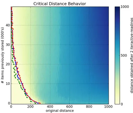
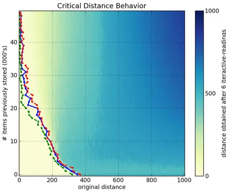
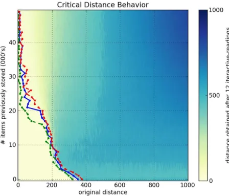
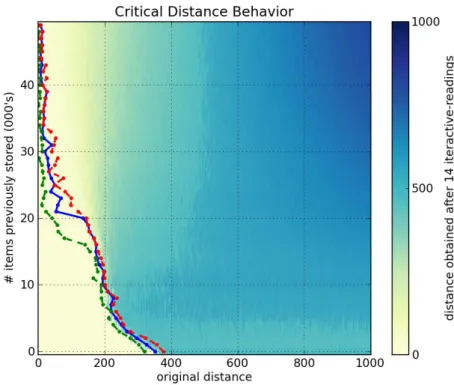
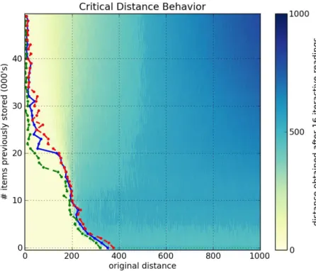
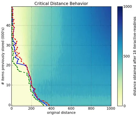
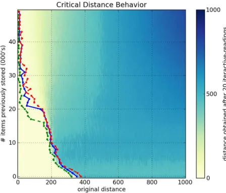
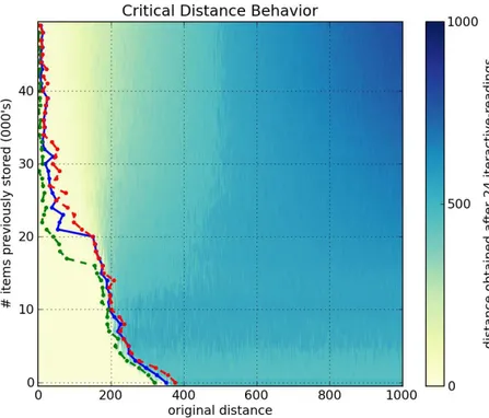
All figures presented below have three colored lines. The green line marks the first occurrence of non-convergence to the exact target bit-string. The red line marks the last occurrence of the convergence to the exact target bitstring. Finally, the blue marks the estimated critical distance, that is where the read output, on average, equals the input distance to the target bitstring. It is an estimation because the critical distance is not exactly defined this way. Critical distance is the point or region in which both divergence and convergence have50% chance to occur (Kanerva,1988[19]). That is, all points before the green line converged, all points after the red line diverged, and the points between these lines sometimes converge and sometimes diverge.

(47)

4.2 influence of iterative-readings in critical distance 27

4.2 influence of iterative-readings in critical distance

The number of iterative-readings is an important parameter of an SDM implementation. When a SDM memory is running a read operation, it doesn’t know if it is converging or diverging. Of course, if at any step of an iterative-reading the output equals the input, that isread(ηx) =ηx, then the operation has converged. But otherwise, the memory does not know whether it is on the right (convergence) track or the wrong (divergence) one. It just returns the bitstring found. And if the output never equals the input, the memory cannot perform the operation forever.

Simulations were done in a 1000and256-dimensional SDM. Both with one million hard-locations, activating (on average) 1,000 hard-locations per operation and writing the target bitstring η only once. The number of random bitstring written in memory ranges from1,000

to50,000, with steps of1,000. Thus, per1,000written,1to40 iterative-readings were executed to each possible distance to the target (from zero to the number of dimensions).

Figures6a,6b,6cand6dshow, respectively, a1000-dimensional SDM checked with a single read,6,10and40iterative-readings. All figures of iterative-readings, from a single read to40 iterative-readings, are available in the appendix.

It is easy to see a huge difference from a single read to more reads, but a small difference from6to10and from10to40iterative-readings. These observations also apply to our tests with the256-dimensional SDM, in Figures7a,7b,7cand7d. As compared to the1000-dimensional SDM, here we have a smaller, more gradual, difference from a single read to more reads, yet a minute difference from6to10and from10to

40iterative-readings.

It is unexpected that, after 40,000 writes in the 1000-dimensional memory, the critical distance is so small. Kanerva[19] showed that this memory capacity is slightly less than100,000items. He defines memory capacity as full at the number of written random bitstrings for which the critical distance is zero.

In the256-dimensional memory, this behavior starts in20,000writes. This is unexpected, since Kanerva’s estimation for this memory is between112,000and137,000random bitstrings stored.

Following these results, due to the number of computations needed in each simulation, all other simulations were done using6 iterative-readings, since40iterative-readings have only a slight improvement in relation to six.

4.3 influence of the number of writes in critical distance

The influence of the number of writes on the critical distance wasn’t analyzed by Kanerva. It is important because, when a random bitstring is seen only once, it is psychologically plausible that it will be forgotten when new bitstrings come. What matters is not exactly the number of writes, but the proportion in the number of times a bitstring was stored in relation to others.

Figures 8a, 8b, 8cand 8d show a1000-dimensional SDM with 1,

(48)

(a)1000-dimensional SDM,1write of target and single read (b)1000-dimensional SDM,1write of target and6iterative-readings

(c)1000-dimensional SDM,1write of target and10iterative-readings (d)1000-dimensional SDM,1write of target and40iterative-readings

Figure6: Influence of number of iterative-readings in a1000-dimensional SDM memory

(49)

(a)256-dimensional SDM,1write of target and single read (b)256-dimensional SDM,1write of target and6iterative-readings

(c)256-dimensional SDM,1write of target and10iterative-readings (d)256-dimensional SDM,1write of target and40iterative-readings

Figure7: Influence of number of iterative-readings in a256-dimensional SDM memory

(50)

Is it easy to see a huge difference from1to2writes. Although the green line has a strange behavior near50,000items stored, the critical distance was much greater than with 1write. From 2to 5to 9, the critical distance starts growing rapidly and slows down near6writes. This makes sense, since it should have a threshold before500bits.

The256-dimensional memory has a similar behavior, but less abrupt, as can be seen in Figures9a,9b,9cand9d. It keeps growing, but slower than a100-dimensional memory. It never crosses the50bits on x-axis in256bits, while the1000-dimensional reaches the200bits on x-axis and almost hit the 400 bits on x-axis in 1000 bits. Percentage wise,

1000-dimension has much more influence than256-dimensional. These figures displays the immense power of reinforcement or re-hearsal: additional writes of a memory item significantly raise the attractor basin (critical distance) for that item.

This behavior is plausible, since the human brain recognizes a pattern quickly when it is used to it. Many times, the patterns appear in differ-ent contexts, giving cues far from the target concept. It is like a chess player, that looks a game and rapidly recognizes what is happening.

4.4 kanerva’s read vs chada’s read

As can be seen in Figures10a,10b,10cand10dfor1000-dimensional SDM memory, and Figures11a,11b,11cand11dfor256-dimensional SDM memory, the Chada’s read operation results in a smaller critical distance when compared to Kanerva’s read operation.

In the256-dimensional memory, both operations are very close when the target is written a single time (Figures11aand11c). However, when writing the target10times, this difference becomes striking (Figures

11band11d).

In the1000-dimensional memory, there is a slightly difference be-tween operations when the target is written once (Figures10aand10c). However, when writing the target10times, the Chada’s read operation behaves very strangely, almost a vertical line (Figure11d), even for a few items written in memory. This is unexpected and quite different from Kanerva’s read.

4.5 unsuccessful attempt

We have also tried an alternative reading method beyond Kanerva’s original one and Chada’s proposal. This was an attempt to explore the properties of the normal distribution. Because exceedingly few adders will have high positive or high negative values (the mean is zero), we attempted to test whether these adders could, by exerting higher relative influence in the model, provide benefits in terms of memory capacity or time to convergence.

(51)

(a)1000-dimensional SDM,1write of target (b)1000-dimensional SDM,2writes of target

(c)1000-dimensional SDM,5writes of target (d)1000-dimensional SDM,9writes of target

Figure8: Influence of number of target writes in a1000-dimensional SDM memory

(52)

(a)256-dimensional SDM,1write of target (b)256-dimensional SDM,2writes of target

(c)256-dimensional SDM,5writes of target (d)256-dimensional SDM,9writes of target

Figure9: Influence of number of target writes in a256-dimensional SDM memory

(53)

(a) Kanerva’s read,1write of target (b) Kanerva’s read,10writes of target

(c) Chada’s read,1write of target (d) Chada’s read,10writes of target

Figure10: Karnerva’s read compared to Chada’s read in a1000-dimensional SDM memory

(54)

(a) Kanerva’s read,1write of target (b) Kanerva’s read,10writes of target

(c) Chada’s read,1write of target

‘

(d) Chada’s read,10writes of target

Figure11: Karnerva’s read compared to Chada’s read in a256-dimensional SDM memory

(55)

4.6 critical distance through function minimization 35

Figure12: Unsuccessful attempt with value of adders to the power of three

4.6 critical distance through function minimization

Let:

• d: be the distance to the target;

• h: be the number of hard-locations activated during read and write operations (this value depends on access radius);

• s: be the number of total stored bitstrings in memory;

• H: be the number of hard-locations in memory;

• w: be the number of times the target bitstring was written in memory;

• θ: be the total of random bitstrings in allhhard-locations activated by a read operation;

• shared(d): be the mean number of shared hard-locations acti-vated by two bitstringsdbits away from each other. One can find some values for a1000-dimensional SDM in Kanerva’s book, Ta-ble7.1, p.63, or the equations to calculate to any SDM in Kanerva (1988[19], Appendix B, p.125).

Suppose a memory with a total of s stored bitstrings. Each written operation actived approximatelyhhard-locations. This way, in average, all written operations together activated a total ofsh hard-locations. This gives an average ofsh/Hrandom bitstrings stored in each hard-location.

(56)

target bitstringη, and h−shared(d)non-shared hard-locations. The

non-shared hard-locations have only random bitstrings stored in them-selves. However, the shared hard-locations have the target bitstring writtenw times, resulting in less random bitstrings. As the average number of bitstrings written in each hard-locations issh/H, we have:

θ = s·h

H ·[h−shared(d)] +

✓

s_·h H −w

◆

·shared(d)

θ = s·h 2

H −w·shared(d)

Suppose our target bitstring’s k-th bit is zero. The read operation will correctly choose bit zero if, and only if, more than half of the bitstrings from the activated hard-locations has k-th bit zero. As each hard-location hassh/Hbitstrings and the read operation activatesh, half of the bitstrings equals toh·sh/(2H) =sh

2

/(2H). Then, to choose the correct bit, we should havePθ

i₌1Xi < sh2/(2H), whereXi is the k-th bit of thei-th bitstring stored in all activated hard-location.

Suppose our target bitstring k-th bit is one. The read operation will choose bit one when more than half of the bitstrings from the activated hard-locations has the k-th bit one. We already seem that halt of the bitstrings issh2/(2H). But this time, as the bit is one and we havew

target bitstrings in eachshared(d), we have to addk·shared(d)to the

sum. This give usw·shared(d) +

Pθ

i₌1Xi> sh2/(2H). Summarizing, we have:

P(wrong|bit=0) = 1−P 0

@

θ(d)

X

i₌1

Xi<

sh2 2H

1

A

P(wrong|bit=1) = P

0

@

θ₍d₎ X

i₌1

Xi<

sh2

2H −w·shared(d)

1

A

We already know thatP(Xi= 1) =P(Xi =0) =0.5. So,P θ i=1Xi ∼

Binomial(θ;0.5), which has meanθ/2and standard deviationpθ/4. The critical distance is the distance where the chance to get near the target is the same as the distance to get away from the target. That is, in critical distance, the probability of choose wrongly the bit times the number of the bits is equal to the original distance to the target. Then, the critical distance is thedthat satisfies equationP(wrong)·n=dor

P(wrong) =d/n.

Using the theorem of total probability, we have:

P(wrong) = P(wrong|bit=0)·P(bit=0) +P(wrong|bit=1)·P(bit=1)

P(wrong) = 1

2·

2

41−P

0

@

θ(d)

X

i=1