Submitted19 February 2016 Accepted 8 June 2016 Published6 July 2016 Corresponding author Lindsay M. Veazey, [email protected]
Academic editor James Reimer
Additional Information and Declarations can be found on page 20
DOI10.7717/peerj.2189
Copyright 2016 Veazey et al.
Distributed under
Creative Commons CC-BY 4.0 OPEN ACCESS
The implementation of rare events
logistic regression to predict the
distribution of mesophotic hard corals
across the main Hawaiian Islands
Lindsay M. Veazey1, Erik C. Franklin2, Christopher Kelley3, John Rooney4,
L. Neil Frazer5and Robert J. Toonen6
1Department of Biology, University of Hawaii at Manoa, Honolulu, HI, United States
2School of Ocean and Earth Science and Technology, University of Hawaii, Hawaii Institute of Marine
Biology, Kaneohe, HI, United States
3The Hawaii Undersea Research Lab, University of Hawaii at Manoa, Honolulu, HI, United States 4Joint Institute for Marine and Atmospheric Research, University of Hawaii at Manoa, Honolulu, HI,
United States
5Department of Geology and Geophysics, University of Hawaii at Manoa, Honolulu, HI, United States 6Hawaii Institute of Marine Biology, University of Hawaii at Manoa, Kaneohe, HI, United States
ABSTRACT
Predictive habitat suitability models are powerful tools for cost-effective, statistically robust assessment of the environmental drivers of species distributions. The aim of this study was to develop predictive habitat suitability models for two genera of scleractinian corals (LeptoserisandMontipora) found within the mesophotic zone across the main Hawaiian Islands. The mesophotic zone (30–180 m) is challenging to reach, and therefore historically understudied, because it falls between the maximum limit of SCUBA divers and the minimum typical working depth of submersible vehicles. Here, we implement a logistic regression with rare events corrections to account for the scarcity of presence observations within the dataset. These corrections reduced the coefficient error and improved overall prediction success (73.6% and 74.3%) for both original regression models. The final models included depth, rugosity, slope, mean current velocity, and wave height as the best environmental covariates for predicting the occurrence of the two genera in the mesophotic zone. Using an objectively selected theta (‘‘presence’’) threshold, the predicted presence probability values (average of 0.051 forLeptoserisand 0.040 forMontipora) were translated to spatially-explicit habitat suitability maps of the main Hawaiian Islands at 25 m grid cell resolution. Our maps are the first of their kind to use extant presence and absence data to examine the habitat preferences of these two dominant mesophotic coral genera across Hawai‘i.
SubjectsEcology, Ecosystem Science, Environmental Sciences, Marine Biology
Keywords Mesophotic, Rare events corrected regression, Species distribution model, Hawaii, Scleractinian corals,Leptoseris,Montipora, Theta threshold selection, Predictive modeling
INTRODUCTION
spatial planning, a management approach that synthesizes information about the location, anthropogenic use, and value of ocean resources to achieve better management practices such as defining marine protected areas and implementing harvesting restrictions (Jackson, Trebitz & Cottingham,2000;Larsen et al.,2004). The creation of spatial predictive models for improved marine planning is a relatively low-cost and non-invasive technique for projecting the effects of present-day human activities on the health and geographic distribution of marine ecosystems.
Defining and managing the biological and physical boundaries of ecosystems is a complicated but essential component of marine spatial planning (McLeod et al.,2005). The heterogeneous nature of ecological datasets can require the time-intensive development of problem-specific ecosystem models (Cramer et al.,2001;Tyedmers, Watson & Pauly, 2005). Scientists frequently use straightforward, easy-to-implement regression methods to analyze complex datasets. The development of software accessible to relative novices has contributed to the growing popularity of regression methods (e.g., Lambert et al.,2005; Tomz, King & Zeng,2003).
Here, we employ a logistic regression with rare events corrections (King & Zeng,2001) to analyze the presence and absence data of two coral genera (LeptoserisandMontipora) and, thus, develop a predictive framework for the geographic mapping of mesophotic coral reef ecosystems (MCEs) across the main Hawaiian Islands. Mesophotic coral ecosystems, located at depths of 30–180 m, are considered to be extensions of shallow reefs because they harbor many of the same reef species present at shallower depths, and are also oases of endemism in their own right (Grigg,2006;Lesser et al.,2010;Kane, Kosaki & Wagner, 2014;Hurley et al.,2016). MCE habitats are formed primarily by macroalgae, sponges, and hard corals tolerant of low light levels (Lesser, Slattery & Leichter,2009). Corals of genus
Montiporacolonize primarily the shallow reef zone (<30 m), but some species, particularly
Montipora capitata(Rooney et al.,2010), are able to extend their settlement into mesophotic depths. Corals of genusLeptoserisconstruct extremely efficient, light-capturing skeletons that facilitate their habitation of the lower mesophotic zone (Kahng et al.,2012) and are considered to be exclusively mesophotic dwellers (Kahng & Kelley,2007).
Ecological studies in the mesophotic zone are sharply limited in contrast to the shallower photic zone more accessible by open circuit SCUBA, but steady advances in diving, computing, and remotely operated vehicle technologies continue to facilitate interdisciplinary mesophotic research (Pyle,2000;Puglise et al.,2009). Mesophotic research in Hawai‘i has been conducted primarily in the ‘Au‘au Channel, Maui, a relatively shallow, semi-enclosed waterway between the islands of Maui and L¯ana‘i that is among the most geographically sheltered and accessible areas in the Hawaiian Archipelago, and, as a result, much of the existing video and photo records of MCEs are from this area. This concentration of historic surveys highlights the importance of creating a pan-Hawai‘i predictive habitat model to identify likely areas of MCEs across unexplored areas of Hawai‘i’s mesophotic zone. Increasing our knowledge about the habitat preferences of the deep extensions of shallow coral species is critical given that approximately 40% of shallow (<20 m) reef-building corals face a heightened extinction risk from the effects of climate change (Carpenter et al.,2008). Here, we model the habitat associations of mesophotic
scleractinian corals because of both their intrinsic biological value as well as their potential to recolonize globally threatened shallow reef areas and serve as a refuge to mobile reef organisms (Bongaerts et al.,2010;Kahng, Copus & Wagner,2014).
Previous research about the environmental variables driving mesophotic scleractinian colonization in Hawai‘i suggests that distinct variation in community structure exists between the upper (30–50 m) and mid to lower mesophotic (50–180 m) depths (Rooney et al., 2010; Kahng et al., 2010; Kahng, Copus & Wagner,2014). Potentially influential environmental variables include photosynthetically active radiation (PAR) levels (Goreau & Goreau,1973;Fricke, Vareschi & Schlichter,1987;Kahng & Kelley,2007;Kahng et al.,2010), isotherms (Grigg,1981;Kahng & Kelley,2007;Rooney et al., 2010), and hard substrate availability (Kahng & Kelley,2007;Costa et al.,2012).Rooney et al.(2010) noted that hard coral abundance declined dramatically below 100 m despite high (>25%) availability of colonizable substrate; this sudden reduction in coral cover occurs at increasingly shallower depths across the northwestern Hawaiian Ridge and may be driven by the synchronously shallower occurrence of isotherms.
Light and temperature intensity (Jokiel & Coles,1977;Rogers,1990), physical stress (e.g., wave energy or uncontrolled tourism) (Dollar,1982;Nyström, Folke & Moberg,2000; Franklin, Jokiel & Donahue,2013), and availability of colonizable substrate (Jokiel et al., 2004;Franklin, Jokiel & Donahue,2013) are known drivers of shallow (<30 m) reef coral distributions across the world. We expect that our model will capture the influence of these abiotic variables on the distribution of mesophotic corals, especially in the shallower mesophotic zone. We speculate that our model may detect unexpected drivers ofLeptoseris
distribution, particularly becauseLeptoserisis known to colonize deeper depths that bear little resemblance to shallow reefs (Lesser, Slattery & Leichter,2009;Rooney et al.,2010). Finally, previous predictive modeling research about the drivers of Hawaiian mesophotic coral colonization identified depth, distance from shore, euphotic depth, and sea surface temperature as potentially influential environmental variables (Costa et al.,2012;Costa et al.,2015). Our novel modeling approach utilizes all observational data (corals present and absent), which we believe will offer more insight into the dynamics that facilitate and inhibit coral colonization across the mesophotic zone.
MATERIALS AND METHODS
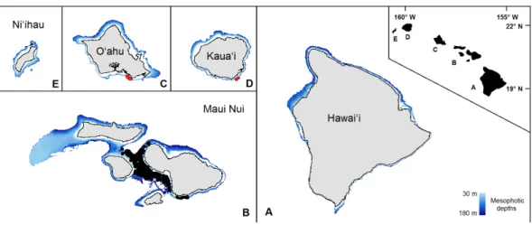
Organismal and environmental dataFigure 1 The mesophotic zone of the main Hawaiian Islands.The study domain, demarcated in blue, encompasses the mesophotic zone (30–180 m in depth) of the main Hawaiian Islands. Black circles are the observations from the pre-existing Maui Nui dataset. Red circles are the previously unprocessed observa-tions in south O‘ahu and southeast Kaua‘i.
Table 1 Number of field observations for each coral genus.
Source No. observations Leptoseris Montipora
O‘ahu 2,645 192 0
Kaua‘i 112 38 3
Maui 19,957 708 791
Total 22,714 938 794
(PIBHMC),2015). PIFSC has used this type of combined analysis, referred to as the random five point overlay method (RFPOM), to process coral reef ecosystem benthic imagery throughout the U.S. Pacific Islands Region since August 2011, and our use of it ensures database consistency with regions processed prior to this study. The CPCe software placed five points randomly on each snapshot, which we then assessed for coral presence. If any of the five points was on coral, that observation was recorded as a ‘‘presence.’’ In an effort to evaluate the accuracy of RFPOM, we counted all corals in 200 randomly selected screengrabs and found that this method misses 2.4% of coral observations recorded in these images. We categorized corals by genus, because both Montipora(Forsman et al., 2010) andLeptoseris(Luck et al.,2013) contain species complexes that remain the subject of taxonomic uncertainty which prevent us from being able to reliably identify corals to the species level from photographs.
We recorded snapshots every 30 s for the duration of each dive video. In addition to an existing database of 40,193 records from dives in the ‘Au‘au Channel, 3517 new snapshots were collected from the additional dives across south O‘ahu and Kaua‘i (Fig. 1). Of these 43,710 total images, 20,980 were discarded because either: (1) crucial observational data were absent; (2) they were redundant due to an extended stationary period; or (3) they fell outside the study depth range of 30–180 m. Of the remaining 22,714 records, we analyzed 2,757 unprocessed images using the RFPOM (Table 1).
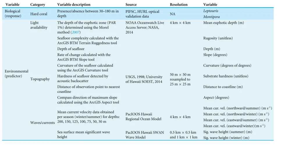
We selected our environmental covariates, listed inTable 2, based on the sufficiency of the data and the potential significance of each variable as an indicator of hard coral habitat suitability (e.g., Dolan et al.,2008; Rooney et al.,2010; Costa et al.,2012). We defined summer and winter seasons as May–September and October–April, respectively (Kay,1994;Rooney et al., 2010). We delineated significant wave height estimates and mean current velocities by season and direction. We extracted and averaged significant wave height data from 144 days per season of twenty-four hour PacIOOS Simulating WAves Nearshore (SWAN) regional wave models estimated values for 2011–2015 (see website: http://oos.soest.Hawaii.edu/las/). Mean current velocity values were available from 0:00–21:00 every three hours for all months from 2013–2015; for each season and direction, 48 mean current velocity values were extracted and averaged from the PacIOOS Regional Ocean Modeling System (see website: http://oos.soest.Hawaii.edu/las/). This model has a 4 km horizontal resolution with 30 vertical levels across seafloor terrain. We sourced monthly MODIS Aqua Chlorophyllaaverages for the year 2012 from the NOAA PIFSC OceanWatch Live Access Server (see website:http://oceanwatch.pifsc.noaa.gov/). Using theMorel(2007) method, we applied the following cubic polynomial equation to obtain logged euphotic depth:
log10Zeu=1.524−0.436x−0.0145x2+0.0186x3, (1)
wherexrepresents the measured Chlorophyllaconcentrations (mg/m3) at sea surface. Euphotic depth is the depth at which the level of photosynthetically active radiation (PAR), a limiting factor for many heterotrophic mesophotic corals, is at 1% of surface PAR. In total, we used 14 environmental predictor variables to shape our model (Table 2) (Figs. S1–S5).
The spatial resolution of the bathymetry data was 50 m×50 m for all islands. We resampled the bathymetry raster to a cell size of 25×25 m consistent with a conservatively estimated±25 m positioning error margin observed at a depth of∼800 m. We estimated an average camera swath value of 3.24 m (range 2.45–4.54 m) based on previous measurements from 19 still image screenshots taken when the submersible was located at different heights above the seafloor. Our geopositional error for the images is±5 m and we can expect that the location data are within a circle with a 10 m diameter. Our observation sampling area is projected out from the location area a distance of≤5 m. Addition of a conservative 5 m observation area buffer to the location error area produces an observational data position of±20 m from the given coordinates of a data point.
Table 2 List of all variables considered for inclusion in our analyses.
Variable Category Variable description Source Resolution Variable
Leptoseris
Biological
(response) Hard coral
Presence/absence between 30–180 m in depth
PIFSC, HURL optical
validation data NA Montipora
Light availability
The depth of the euphotic zone (PAR 1%) determined using the Morel method (2007)
NOAA Oceanwatch Live Access Server; NASA, 2014
4 km×4 km Mean euphotic depth (m)
Seafloor complexity calculated with the ArcGIS BTM Terrain Ruggedness tool
Rugosity (unitless)
Depth of seafloor Depth (m)
Rate of change calculated with the ArcGIS BTM Slope tool
Slope (degrees)
Curvature of the seafloor calculated using the ArcGIS Curvature tool
Curvature (degrees of degrees)
Hardness of seafloor detected by acoustic backscatter
Substrate hardness (unitless)
Distance of observation point to nearest coastline
Distance to coastline (m) Topography
Compass direction of maximum slope calculated using the ArcGIS Aspect tool
USGS, 1998; University of Hawaii SOEST, 2014
50 m×50 m resampled to 25 m×25 m
Aspect (degrees)
Mean cur. vel. (northward/summer) (m s-1)
Mean cur. vel. (northward/winter) (m s-1)
Mean cur. vel. (eastward/summer) (m s-1)
Mean current velocity data obtained per season (winter/summer) for depths: 200, 150, 125, 100, 75, 50, 30 m
PacIOOS Hawaii
Regional Ocean Model 4 km×4 km
Mean cur. vel. (eastward/winter)(m s-1)
Sig. wave height (summer) (m) Environmental
(predictor)
Waves/currents
Sea surface mean significant wave height
PacIOOS Hawaii SWAN Wave Model
0.5 km×0.5 km
and 1 km×1 km Sig. wave height (winter) (m)
Regression methods
In describing the relationship between a response variable and one or more predictor variables, we use a logistic regression model because the response variable is dichotomous (Hosmer & Lemeshow,2004). The ordinary logistic regression (OLR) model is defined as:
θ=expit(µ)= 1
1+exp(−µ), (2)
whereθ is the probability that the species of interest is present (y=1), and 1−θ is the probability it is absent (y=0). The logit function is the inverse of the expit function, and
logit(θ)=µ=β0+β1x1+ ··· +βnxn (3)
is the linear sum of predictor variables, x1,x2,..., xn, with interceptβ0 andregression
coefficientsβ1,β2,...,βn. In the language of generalized linear models (GLM), OLR is
said to have the logit function as its link function and the expit function as its inverse link function. Logistic regression provides a straightforward, meaningful interpretation of the relationship between a dichotomous dependent variableyand a set of predictor variables (Allison,2001).
Despite the popularity of OLR, it may yield extremely biased results when an imbalance exists in the proportion of the response variable data (e.g., such as in our case, when
y=0≫y=1) (Van Den Eeckhaut et al.,2006).King & Zeng (2001) coined the term ‘‘rare events logistic regression’’ to describe their corrective methodology in dealing with unbalanced binary event data:
1. The first step requires the selection of a representative sample. Though researchers generally prefer to work with more uniform response data (e.g.,Liu et al., 2005), selection of an unusually high proportion of the rare event (in this case, y=1) to ‘‘balance’’ the dataset and increaseθ estimates will yield nonsensical results. We divided the data in half to create our training and testing datasets and checked that each set of observations had an approximately equal proportion (y) of presence observations to better reflect the ‘‘true state’’ of the full dataset.
2. The second step rectifies any bias that might be introduced when dividing the dataset. This prior correction on the intercept (β0) can be calculated as:
ˆ
β0=β˜0−ln
1−τ τ
y
1−y
; (4)
here, βˆ0 is the corrected intercept, β˜0 is the uncorrected intercept,τ is the true
proportion of 1s in the population; andy is the observed proportion of 1s in the training sample.
3. The third step rectifies any underestimation of the probabilities of the independent variablesβ1...nfrom the substitution of the intercept value, obtained as:
P(yi=1)=˜θi+Ci, (5)
where the correction factorCiis given by:
whereX is a 1×(n+1) vector of values for each independent variableβi,X′ isthe
transpose ofX, andV(β˜i) is the variance covariance matrix. We obtained the improved
probability estimates through estimation ofβi viaβ˜i , thereby considered ‘‘mostly’’
Bayesian (King & Zeng,2001). Our priors in this case would be uninformative, which means that we lack sufficient knowledge to estimate the probability distributions of our data and our parameter of interest,θ. This is often the case when working with sparse ecological datasets. As the uninformative prior for a regression coefficient with domain (∞,−∞) is uniform, a full Bayesian estimation with uninformative priors is equivalent to a traditional logistic regression. Therefore, this correction is effectively a correction to the approximate Bayesian estimator, and its addition improves our regression by lowering the mean squared error of our estimates. We implemented this rare events logistic regression using the ‘Zelig’ package run in R (Imai, King & Lau, 2008;Choirat et al.,2015).
We constructed a correlation scatterplot matrix per coral genus to observe correlation levels between all variables. In choosing which highly correlated variables to exclude from the analyses, we followed the criteria outlined byDancey & Reidy(2004) andTabachnick & Fidell(1996), who suggest a cutoff correlation value of 0.7. Only mean significant wave height parsed by season consistently overreached this threshold; the covariate that was least correlated with the response variable was removed. We excluded predictors that lacked a clear distribution pattern or correlated minimally (<0.05) with the response variable.
One of the more studied habitat preferences ofLeptoserisandMontiporais the influence of depth on their distribution (Rooney et al.,2010;Costa et al.,2012;Kahng et al.,2010). Increasing depths often correlate with greater distance from shore. The inclusion of squared terms (e.g.,x2=x12) in our regression equation expit(θ)=β0+β1x1+ ··· +βnxn permits
the logistic curve to reflect the bell curve shape expected in plotting the distribution of these animals across a range of depths or distance from shore. In order to account for these trends, we added Depth Squared and Distance Squared as potential variables for consideration in our final model. As depth or distance increases, its square increases even more rapidly, allowing the squared term to eventually dominate and ‘‘pull down’’ the probability curve.
We withheld 50% of our information per genus as testing (i.e., validation) data. Using the remaining 50% (our training data), we performed the rare events corrected logistic regression described above. Using an exhaustive iterative algorithm (Calcagno, Mazancourt & Claire,2010), we modeled all possible combinations of included covariates. We ranked models using the corrected Akaike information criterion (AICc) (Hurvich & Tsai,1989), which is considered an excellent comparative measurement of model strength, especially for sparse datasets. For both genera, the models with the lowest (lowest=best) AICc scores were lower than the ‘‘second best’’ AICc scores by at least 2 (i.e.,1AICc≥2), indicating strong preference for the best model (e.g., (Hayward et al.,2007)).
In an ideal and unrealistic study, all biotic and abiotic components of a model would be homogenous and evenly distributed across a sampling space. Our sampling design includes overlapping submarine dive tracks and the inherent heterogeneity of the marine environment, which could problematically violate our model’s underlying assumption
Table 3 Summary statistics for theoretical semivariogram models.
Genus Sum of squares Inputσ2 Inputψ Actualσ2 Actualψ Actualτ2
Leptoseris 2940.671 0.055 218 0.051 206.909 0
Montipora 14013.610 0.020 390 0.032 390.000 0.003
regarding the independence of our biological and environmental data. We removed all instances of pseudoreplication (multiple observations in one grid cell) when we assigned each grid cell to a category of ‘‘corals present’’ or ‘‘corals absent.’’ After we removed subsampling within our observational data, we checked for the presence of clustering, or spatial autocorrelation, within these data. Uncorrected spatial autocorrelation between observational data points confounds and undermines any biological inferences drawn from model predictions.
We checked small-scale, local spatial autocorrelation using Geary’s C statistic (Geary, 1954), based on the deviations in the responses of observation points with one another:
C=n−1 2S0
X
i
X
j
wij(xi−xj)2
P
i(xi−x)2
. (7)
Here, xis the variable of interest,i andj are locations (wherei6=j),wijrepresents the
components of the weight matrix, andS0is the sum of the components of the weight
matrix. Geary’s C ranges from 0 (maximal positive autocorrelation) to 2 for high negative autocorrelation. In the absence of autocorrelation, its expectation is 1 (Sokal & Oden,1978). We also examined global spatial autocorrelation using Moran’s I statistic, which measures cross-products of deviations from the mean (Moran,1950):
I= n S0
X
i
X
j
wij(xi−x)(xj−x)
X
i
(xi−x)2
. (8)
Moran’s I values generally range from –1 to 1, with 0 as the expectation when no spatial autocorrelation is present.
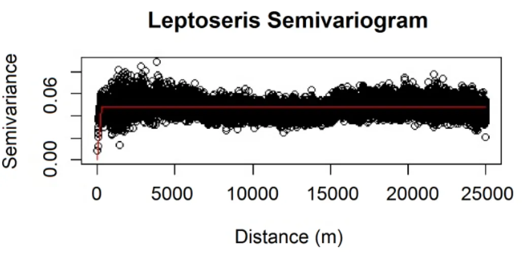
We also verified the spatial independence of our observational point data using a semivariogram, which is a graphical method of quantifying spatial correlation in a set of points (Figs. 2–3). We selected our theoretical semivariogram to fit the empirical semivariance using the ordinary least squares (OLS) method (Jian, Olea & Yu,1996;Kendall et al.,2005). The spherical model had the best quantitative fit based on OLS estimates (Table 3). For each dataset, the low thresholds at which semivariance stopped increasing indicated the almost complete absence of spatial autocorrelation for each genus.
Model assessment
Figure 2 Modeled spherical semivariogram for Leptoseris.
Figure 3 Modeled spherical semivariogram for Montipora.
applicability to logistic regressions and are therefore ignored (Menard,2000;Peng, Lee & Ingersoll,2002). Sample size and selected threshold largely influence the results of the Hosmer and Lemeshow goodness-of-fit test (Hosmer et al.,1997). Accordingly, we use model classification accuracy as a second measure of goodness-of-fit (in addition to1AICc). We want to maximize true positives (TP) and true negatives (TN) while minimizing false positives (FP) and false negatives (FN). The sensitivity-specificity sum maximization approach (Cantor et al.,1999) therefore maximizes
SSmax=
TP TP+FN +
TN
TN+FP, (9)
which is equivalent to finding the point on the ROC (receiver operating characteristics) curve at which the tangent slope is 1, indicating the optimal cutoff point at which ‘‘cost’’ (here, the number of FN and FP) and ‘‘benefit’’ (the number of TN and TP) is balanced. We chose this technique because we aim to identify regions devoid of hard corals as well as regions deemed potentially suitable for habitation.
ROC curves plot the true positive test rate against the false positive test rate across different theta cutoff points (Hadley & McNeil,1982). We calculated values for sensitivity and specificity for threshold increments of 0.005±1 standard deviation of the rounded mean for each model. Because each theta threshold value varied based on the genus and model, the threshold-independent area under the curve (AUC) test statistic best reflects the predictive accuracy of the model.
In addition to creating ROC curves, we also took into account the overall prediction success of each model, given as:
OPS= TP+TN
TP+TN+FP+FN. (10)
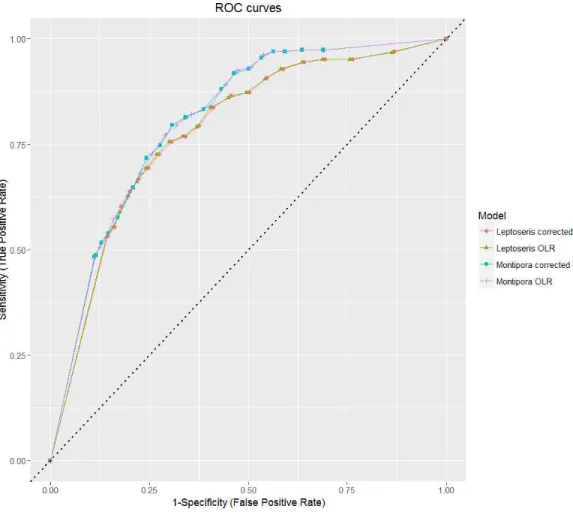
Overall prediction success is a measure of total correct classification of both present and absent observations. While this is a good final assessment of model classification error, consideration of the prediction success alone is not a viable evaluation method when binary data is highly imbalanced, as a value given by this method may primarily represent model success in identifying the most common observation type (Fielding & Bell,1997). We plot-ted our sensitivity and specificity values on a ROC curve to show how each model performed relative to chance (Fig. 4). All models fall in the range 0.7≤AUC < 0.9, which indicates good discrimination and reliability of model predictions (Hosmer & Lemeshow,2004).
We also created maps of individual and summed predicted occurrence probabilities of both coral genera across the main Hawaiian Islands and ran a hotspot analysis using the ArcGIS Getis-OrdG∗i Hotspot Analysis tool. We constructed a polygon fishnet composed of 1×1 km cells which encompassed all islands. We summed each 25×25 m raster cell value for probability ofLeptoserisoccurrence and probability ofMontiporaoccurrence. We performed a spatial join of raster cell values within each polygon for an average value of summed probabilities. The Getis-OrdG∗i statistic identifies clusters within these polygons that display values higher in magnitude than random chance would permit. The Getis-Ord local statistic is given as:
G∗i =
n
X
j=1
wi,jxj−X n
X
j=1
wi,j
S s
1 n−1
nPn
j=1wi2,j−
Pn
j=1wi,j
2
. (11)
Here, wi,j represents the spatial weights between features i and j; n represents the
total number of features;xj is the attribute value for feature j; X =n1 n
X
j=1
xj; and
S= v u u t 1 n n X
j=1
Figure 4 ROC curves for all models.AUC values for all models fall in between 0.7 and 0.9, which indi-cates predictive reliability. The dashed line from (0, 0) to (1, 1) indiindi-cates the null threshold at which model performance is considered unacceptable (<0.5).
RESULTS
Geary’sC test statistic is a measure of local (small-scale) spatial autocorrelation; in the absence of correlation, 1 is the expected value of Geary’s C. Moran’s I is a measure of global (large-scale) spatial autocorrelation; in the absence of correlation, a value of 0 is expected for the Moran’sI test statistic. For ourLeptoserisdataset, Geary’sC=0.990; for ourMontiporadataset, Geary’sC=0.996. For ourLeptoserisdataset, Moran’sI =0.006; for our Montiporadataset, Moran’sI =0.003. These values do not indicate any local clustering or global spatial autocorrelation within either dataset. We observed negligible levels of autocorrelation up to∼100 m forMontipora(Fig. 3). By ensuring that spatial autocorrelation is not present in our data, we do not violate the assumption that our response data are independently observed, which enables us to draw robust conclusions about the ecological factors influencing the distribution of these coral genera within the mesophotic zone across the main Hawaiian Islands.
The OLR covariate coefficients were modified using the rare events corrections proposed byKing & Zeng(2001), resulting in a change in predictive power (Table 4). Rare events
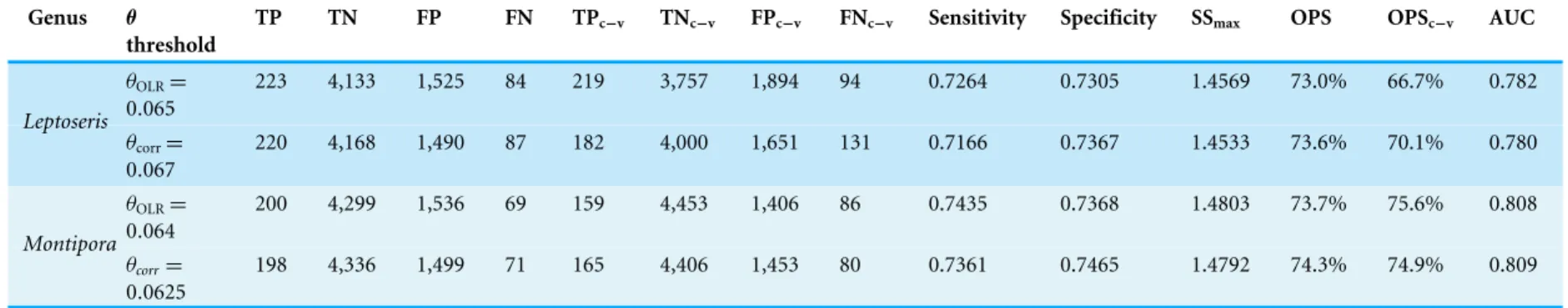
Table 4 Predictive models output.Results by genus: theta threshold subscripts indicate model type and training and validation (c-v) outputs. Sensitivity and specificity totals apply to training data only.
Genus θ
threshold
TP TN FP FN TPc−v TNc−v FPc−v FNc−v Sensitivity Specificity SSmax OPS OPSc−v AUC
θOLR=
0.065
223 4,133 1,525 84 219 3,757 1,894 94 0.7264 0.7305 1.4569 73.0% 66.7% 0.782
Leptoseris θcorr=
0.067
220 4,168 1,490 87 182 4,000 1,651 131 0.7166 0.7367 1.4533 73.6% 70.1% 0.780
θOLR=
0.064
200 4,299 1,536 69 159 4,453 1,406 86 0.7435 0.7368 1.4803 73.7% 75.6% 0.808
Montipora θcorr=
0.0625
198 4,336 1,499 71 165 4,406 1,453 80 0.7361 0.7465 1.4792 74.3% 74.9% 0.809
V
eaze
y
e
t
al.
(2016),
P
eerJ
,
DOI
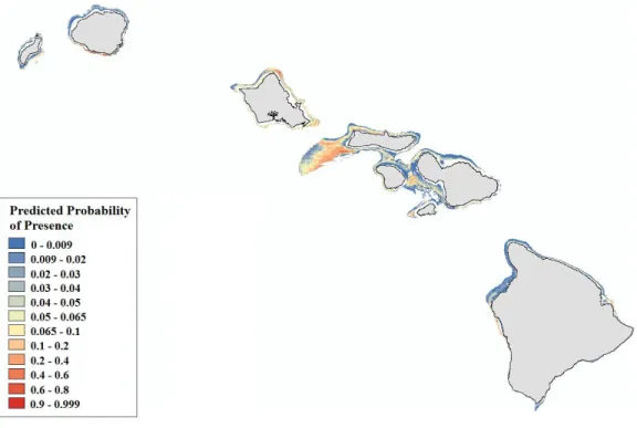
Figure 5 Modeled area of suitable habitat forLeptoseris. Probability of presence is depicted along a color gradient ranging from red (1; most suitable) to blue (0; least suitable).
corrected models usually performed better than the uncorrected models, in terms of improved specificity and prediction success. Our sensitivity values for both corrected models were slightly lower than the corresponding OLR sensitivities, but in each case, specificity and prediction success values were improved. Additionally, standard errors of the coefficient estimates were lower for corrected models than for uncorrected models (Tables S1–S4).
Leptoseriscorals inhabit mesophotic regions with high slope and rugosity values, high to moderate perennial current flow, and their occurrence peaks around 100 m (Table S3,
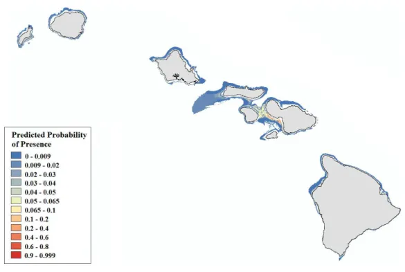
Figs. S6–S10).Montiporacorals peak in occurrence around 60 m and colonize regions less exposed to high energy winter swells (Table S4,Figs. S11–S12). Predicted presence probability values (θ) averaged 0.051 forLeptoserisand 0.040 forMontiporamodels in the validation data (Figs. 5–6). These values agree well with the actual presence frequencies in that data (0.052, 0.042). To better interpret these realistically low theta values, we chose a theta threshold to transform the probability estimates to presence/absence values. This is standard practice when examining the results of a rare events logistic regression, but less common when performing OLR (Liu et al.,2005). Objective selection of a theta threshold on a per-model basis is more scientifically sound than, for example, an arbitrary assignment of 0.5 (Cramer,2003). The transformed model is valid if a threshold value yields a high percentage of correctly classified observations and a low number of FP and FN observations (Gobin, Campling & Feyen,2001). We selected an appropriate threshold for each model (Table 4) in order to maximizeSSmax(Liu et al.,2005).
Figure 6 Modeled area of suitable habitat forMontipora. Probability of presence is depicted along a color gradient ranging from red (1; most suitable) to blue (0; least suitable).
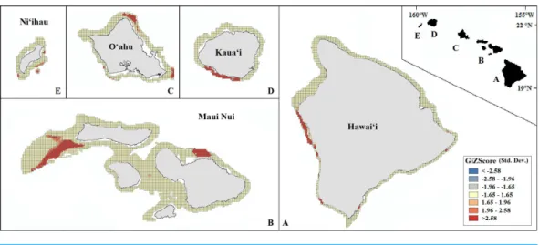
Our final hotspot maps show the results of our analysis forLeptoseris, Montipora,and both genera combined across all islands (Figs. 7–9). We show hotspots of habitat suitability for both coral genera in red for areas of highest suitability and blue for areas of lowest suitability. We identify a cell as a hotspot when the sum of its value and the values of its nearest neighbors is much higher or lower than the mean over all cells. When the local sum of a cluster is very different from the expected value, a statistically significant hotspot is identified (G∗i statistic≥1.96 orG∗i statistic≤ −1.96). Neither genus clearly dominated the summed probabilities hotspot identification across any of the islands. LargeLeptoseris
hotspots were identified in southwest Moloka‘i, northeast O‘ahu, west Hawai‘i, and the central ‘Au‘au Channel.Montipora hotspots were identified in east Ni‘ihau, southwest Kaua‘i, west and south O‘ahu, west Hawai‘i, and the central ‘Au‘au Channel.
DISCUSSION
In this study, we used logistic regression with rare events corrections to predict the habitat preferences of two dominant scleractinian coral genera across the entire mesophotic zone surrounding the main Hawaiian Islands. The habitat preferences of Montiporain the mesophotic zone appear distinct from those ofLeptoseris.Montiporaprefers the middle mesophotic zone (50–80 m) of reefs less exposed to high-energy winter swells.Leptoseris
Figure 7 Mapped result of our Getis-OrdG∗
i hotspot analysis performed for probability estimates
ofLeptoserisoccurrence. A significant hotspot is <−1.96 or >1.96; here, all hotspots are shown in red (>1.96) or blue (<−1.96).
Figure 8 Mapped result of our Getis-OrdG∗
i hotspot analysis performed for probability estimates
ofMontiporaoccurrence.A significant hotspot is <−1.96 or >1.96; here, all hotspots are shown in red (>1.96) or blue (<−1.96).
Important environmental covariates
PredictedMontiporapresence peaks at about 60 m (median occurrence probability=7.5%);
Leptoserispresence peaks at about 100 m (median occurrence probability=7.5%). These predictions are consistent with the inferences of Rooney et al.(2010), which separates mesophotic reefs into three distinct depth sections: upper (30–50 m), branching/plate dominated (50–80 m), andLeptoserisdominated (≥80 m). The depth at which suitability peaks forLeptoserisoccurs at a range where steep ridges and drop-offs are plentiful in our study region, and therefore the mean preferred depth may be prone to slight overestimation.
In addition to depth, four environmental covariates appeared to influence the distribution ofLeptoseris: rugosity, slope, summer mean current velocity (northward), and winter mean current velocity (eastward). Scleractinians easily colonize environments
Figure 9 Mapped result of our Getis-OrdG∗
i hotspot analysis performed for summed probability
estimates ofLeptoserisandMontiporaoccurrence. A significant hotspot is <−1.96 or >1.96; here, all hotspots are shown in red (>1.96).
that are relatively calm and rugose due to the larger amount of available surface area, and this positive correlation was reflected in our model.Leptoserishabitat preference was also positively associated with slope, which was not observed forMontipora.Corals that inhabit the upper mesophotic zone may be more susceptible to damage from debris displaced by high wave energy, and are therefore less likely to colonize steep slopes (e.g.,Harmelin-Vivien & Laboute,1986;Bridge & Guinotte,2013). The deeper distribution ofLeptoserismay protect it from damage related to wave intensity, allowing it to colonize slopes (e.g.,White et al., 2013). Another possibility is that the model is picking up drop-offs from masses accreted during the last glacial maximum. These steep drop-offs are present between 90–120 m in the
Leptoseris-dominated lower mesophotic zone (Yokoyama et al.,2001;Webster et al.,2004).
Leptoserisalso favors well-flushed areas exposed to year-round moderate current flow (i.e., up to 0.3 m/s). The plate-like morphology ofLeptoseriscorals effectively boosts sunlight capture by its symbiotic zooxanthellae and zooplankton capture by the corals themselves, but it also makes the coral vulnerable to smothering by sediment accumulation (Bak, Nieuwland & Meesters,2005;Bongaerts et al.,2010;Marcelino et al.,2013). The success of
Leptoseriscorals in areas of moderate current flow may be related to the improbability of sediment settlement and accumulation. While the model did not capture the same effect of current flow onMontipora distribution, we recognize that the morphology of someMontiporaspecies is extremely similar to that ofLeptoseris.We do not expect either genus to readily colonize highly turbid regions, especially given that certain species of heterotrophic Montipora are thought to exploit strong currents to meet their energy requirements (Grottoli, Rodrigues & Palardy,2006;Rooney et al.,2010).
well as across small rock fragments strewn across a sand flat, which would be obscured by the softness of the surrounding benthos. We can conclude that measurements of benthic hardness are not detailed enough for predictive modeling purposes at a 25×25 m resolution.
We emphasize that the purpose of this study was to build a pan-Hawai‘i predictive habitat map for two dominant coral genera within the mesophotic zone. Because the scope of this study included all main Hawaiian Islands, we were constrained by the coarseness of available full-coverage environmental data. As we build on this analysis, we plan to use our maps to identify areas of interest for further study at higher resolution and to include additional variables currently only available in certain regions, such as light intensity and temperature at depth. For example, our predictive and hotspot maps identify Penguin Bank (southwest Moloka‘i) as particularly suitable forLeptoseriscolonization, which has not been verified by video or photo records. High resolution backscatter data (1×1 m) exist for this region, and incorporation of these data into new analyses of subsets of our study area may refine our conclusions.
Error sources and model reliability
We examined two types of error (false negatives and false positives) and analyzed our models without giving preference to either one. This approach is widely accepted as the best method of overall error minimization (e.g.,Liu et al.,2005;Fielding & Bell,1997). Rare events corrected models for bothLeptoserisandMontipora achieved levels of specificity and sensitivity well above the null, indicating good predictive power. Additionally, both models attained about 74% overall prediction success. We assumed coral detectability was constant across the study region and that we can therefore consider the true absence observations to be reliable indicators of a potentially unsuitable habitat for corals. For each genus, the model tended to slightly over-predict presence observations; large numbers of false positives lowered sensitivity values. This is inevitable in the analysis of severely imbalanced or sparse binary data; the ongoing addition of presence observations to the dataset will improve overall model classification accuracy.
While the consistent identification of southern coastal areas as suitable is reliable, the comparatively infrequent selection of northern coasts is likely due to the source of the model-building observations. The vast majority of mesophotic exploration has been along southern coastlines, which is often where waters are calmest in Hawai‘i. It is speculated that because mesophotic corals are more shielded from winter long-period wave energy than their shallow water counterparts, they are able to flourish at depth along northern coastlines (Grigg,1998;Rooney et al.,2010). The addition of data sourced from northern expeditions would likely improve predictive power of the model across north-facing coastlines (Alin,2010).
We acknowledge that the original data were not collected in a standardized fashion (e.g., variation in vessel traveling speed or differences in data collection vessel and/or quality). Our careful exclusion of overlapping observation points within each 25×25 m rectified this sampling design flaw as much as possible and eliminated pseudoreplication.
Distinctions between coral genera
Our Montiporamodel was simpler than theLeptoserismodel in that the only variable included other than depth was winter significant wave height. Though uncertainty was highest at lower values of significant wave height,Montiporademonstrated a preference in colonizing habitats that experience lower significant wave height during winter. This preference contrasts withMontipora species in shallow waters that were more likely to be observed in higher wave height environments (Franklin, Jokiel & Donahue,2013). This likely influenced the inability of the model to identify any suitable habitat around Ni‘ihau, where the average winter significant wave height equaled 1.78 m, almost double the mean significant wave height of our model training data (0.91 m). Though mesophotic corals are generally thought to be exempt from the growth limitations faced by shallow water corals in regions of high wave energy, prolonged wave intensity has been shown to negatively affect the colonization of upper mesophotic scleractinians, especially in sloping areas prone to debris avalanches (Bridge & Guinotte,2013;Kahng, Copus & Wagner,2014). Continuation of this work might include a more in-depth examination of the relationship of this coral genus with the combined effects of slope of available substrate and exposure to wave energy.
We found no records ofMontiporapresence when processing our O‘ahu dataset, which probably contributed to the very low predicted mean probability ofMontiporaoccurrence there (0.1%). We believe this is due in part to the sampling pattern across south O‘ahu; we recorded 62.3% of all observations processed for this region at a depth of 75 m or greater.Montiporaprevalence is greater in the upper-to-middle mesophotic zone, and the relative deepness of the O‘ahu dives likely influenced their nonappearance in this portion of the dataset. We emphasize that the dearth ofMontiporaobservations around O‘ahu is an artifact of the dataset we used to construct our model;Montiporacorals have been observed in mesophotic depths across O‘ahu (e.g.,Fig. 4B,Rooney et al.,2010). The mean significant wave height across the mesophotic zone was lower across the southern and western coasts (1.50 m) than that observed across the northern and eastern coasts (2.37 m) of the island. As at Ni‘ihau, we assume that this high northern and eastern average height, coupled with the absence ofMontiporapresences in O‘ahu in the training dataset, greatly impacted our model’s ability to detect areas of suitable habitat around the island. The results of our Getis–OrdG∗
i Hotspot Analysis corroborate the findings ofCosta et al.(2015), who used
Maximum Entropy software to predict the highest occurrence probability ofLeptoserisand
drivers influence the distributions of shallow corals, the occurrence patterns of mesophotic corals may reflect a more stable environment with an increased influence of biotic factors such as interspecific competition in a habitat zone with limited light and space resources available.
CONCLUSIONS
We implemented a rare events corrected logistic regression to determine the most influential environmental predictors ofMontiporaandLeptoseriscolonization in the mesophotic zone. Habitat preference differences between these genera appear distinct and multi-faceted.
Montipora thrives in the middle mesophotic zone in areas sheltered from high intensity winter swells, whileLeptoseristends to colonize steep, rugose, well-flushed areas in the lower mesophotic zone. Improved understanding of the distribution of mesophotic corals will enable resource managers to propose the construction of seafloor power cables and other offshore infrastructure in areas less likely to contain coral communities. Results will likewise facilitate efforts to protect these communities by supplementing scientific dive planning and strategies for conservation, such as marine spatial planning.
ACKNOWLEDGEMENTS
Authors thank the many staff members of HURL, PIFSC, and SOEST who helped acquire and process our data. L.V. thanks Dr. David Hondula (Researcher at Arizona State University) for his dedicated GIS instruction. We dedicate this manuscript to the memory of our coauthor, Dr. John Rooney.A hui hou, John. This manuscript is HIMB contribution #1662 and SOEST contribution #1947.
ADDITIONAL INFORMATION AND DECLARATIONS
Funding
Funding for this research was provided by the NOAA Coral Reef Conservation Program grant no. NA14NOS4820092. The funders had no role in study design, data collection and analysis, decision to publish, or preparation of the manuscript.
Grant Disclosures
The following grant information was disclosed by the authors: NOAA Coral Reef Conservation Program: NA14NOS4820092.
Competing Interests
Robert Toonen is as an Academic Editor for PeerJ.
Author Contributions
• Lindsay M. Veazey conceived and designed the experiments, performed the experiments, analyzed the data, contributed reagents/materials/analysis tools, wrote the paper, prepared figures and/or tables, reviewed drafts of the paper.
• Erik C. Franklin conceived and designed the experiments, analyzed the data, contributed reagents/materials/analysis tools, reviewed drafts of the paper.
• Christopher Kelley, John Rooney and Robert J. Toonen contributed reagents/material-s/analysis tools, reviewed drafts of the paper.
• L. Neil Frazer conceived and designed the experiments, contributed reagents/material-s/analysis tools, reviewed drafts of the paper.
Data Deposition
The following information was supplied regarding data availability:
The data sets and raw code are included in theSupplemental Information.
Supplemental Information
Supplemental information for this article can be found online athttp://dx.doi.org/10.7717/ peerj.2189#supplemental-information.
REFERENCES
Alin A. 2010.Multicollinearity.Wiley Interdisciplinary Reviews: Computational Statistics 2:370–374DOI 10.1002/wics.84.
Allison PD. 2001.Logistic regression using the SAS system: theory and application. New York: Wiley Interscience, 288 pp.
Bak RPM, Nieuwland G, Meesters EH. 2005.Coral reef crisis indeep and shallow reefs: 30 years of constancy and change in reefs ofcuracao and bonaire.Coral Reefs 24:475–479DOI 10.1007/s00338-005-0009-1.
Bongaerts P, Ridgway T, Sampayo EM, Hoegh-Guldberg O. 2010.Assessing the ’deep reef refugia’ hypothesis: focus on caribbean reefs.Coral Reefs29:309–327
DOI 10.1007/s00338-009-0581-x.
Bridge T, Guinotte J. 2013.Mesophotic coral reef ecosystems inthe great barrier reef world heritage area: their potential distribution and possible role as refugia from disturbance. Research Publication no. 109. Townsville: Great Barrier Reef Marine Park Authority.
Calcagno V, Mazancourt, Claire D. 2010.glmulti: an R package foreasy automated model selection with (generalized) linear models.The Journal of Statistical Software 34:1–29DOI 10.18637/jss.v034.i12.
Cantor SB, Sun CC, Torturer-Luna G, Richards-Koru R, Follen M. 1999.A comparison of C/B ratios from studies using receiver operating characteristic curve analysis.
Journal of Clinical Epidemiology52:885–892DOI 10.1016/S0895-4356(99)00075-X.
Carpenter KE, Abrar M, Aeby G, Aronson RB, Banks S, Bruckner A, Chiriboga A, Cortés J, Delbeek JC, DeVantier L, Edgar GJ. 2008.One-third of reef-building corals face elevated extinction risk from climate change and local impacts.Science 321(5888):560–563DOI 10.1126/science.1159196.
Choirat C, Honaker J, Imai K, King G, Lau O. 2015.Zelig: everyone’s statistical software, Version 5.0–3.Available athttp:// ZeligProject.org.
channel, Hawai‘i. NOAA Technical Memorandum NOS NCCOS 149. NOAA/Na-tional Centers for Coastal Ocean Science, Silver Spring, 1–44.
Costa B, Kendall MS, Parrish FA, Rooney J, Boland RC, Chow M, Lecky J, Montgomery A, Spalding H. 2015.Identifying suitable locations for mesophotic hard corals offshore of Maui, Hawai‘i.PLoS ONE10(7):e0130285
DOI 10.1371/journal.pone.0130285.
Cramer JS. 2003.Logit models: from economics and other fields. Cambridge University Press, 66–67.
Cramer W, Bondeau A, Woodward FI, Prentice IC, Betts RA, Brovkin V, Cox PM, Fisher V, Foley JA, Friend AD, Kucharik C, Lomas MR, Ramankutty N, Sitch S, Smith B, White A, Young-Molling C. 2001.Global response of ter-restrial ecosystem structure and function to CO2and climate change:
results-from six dynamic global vegetation models.Global Change Biology7:357–373
DOI 10.1046/j.1365-2486.2001.00383.x.
Crowder L, Norse E. 2008.Essential ecological insights for marine ecosystem-based management and marine spatial planning.Marine Policy32:772–778
DOI 10.1016/j.marpol.2008.03.012.
Dancey C, Reidy J. 2004.Statistics Without Maths for Psychology. New York: Pearson Education Limited.
Dolan M, Grehan A, Gunhan J, Brown C. 2008.Modelling the local distribution of cold-water corals in relation to bathymetric variables: adding spatial context to deep-sea video data.Deep Sea Research Part I: Oceanographic Research Papers56:1564–1579
DOI 10.1016/j.dsr.2008.06.010.
Dollar SJ. 1982.Wave stress and coral community structure in Hawaii.Coral Reefs 1:71–81DOI 10.1007/BF00301688.
Douvere F. 2008.The importance of marine spatial planning in advancing ecosystem-based sea use management.Marine Policy32:762–771
DOI 10.1016/j.marpol.2008.03.021.
Fielding AH, Bell JF. 1997.A review of methods for the assessment of prediction errors in conservation presence/absence models.Environmental Conservation24:38–49
DOI 10.1017/S0376892997000088.
Foley M, Halpern B, Fiorenza M, Armsby M, Caldwell M, Crain C, Prahler E, Rohr N, Sivas D, Beck M, Carr M, Crowder L, Duffy J, Hacker S, McLeod K, Palumbi S, Peterson C, Regan H, Ruckelshaus M, Sandifer P, Steneck R. 2010. Guidinge-cological principles for marine spatial planning.Marine Policy34:955–966
DOI 10.1016/j.marpol.2010.02.001.
Forsman ZH, Concepcion GT, Haverkort RD, Shaw RW, Maragos JE, Toonen RJ. 2010.
Ecomorph or endangered coral? DNA and microstructure reveal Hawaiian species complexes: montipora dilatata/flabellata/turgescens and m. patula/verrilli.PLoS ONE 5(12):e15021DOI 10.1371/journal.pone.0015021.
Franklin EC, Jokiel PL, Donahue MJ. 2013.Predictive modeling of coral distribution and abundance in the Hawaiian islands.Marine Ecology Progress Series481:121–132
DOI 10.3354/meps10252.
Fricke HW, Vareschi E, Schlichter D. 1987.Photoecology of the coralLeptoseris fragilis
in the red sea twilight zone (an experimental study by submersible).Oecologia 73:371–381DOI 10.1007/BF00385253.
Geary R. 1954.The contiguity ratio and statistical mapping.The Incorporated Statistician 5:115–146DOI 10.2307/2986645.
Gobin A, Campling P, Feyen J. 2001.Logistic modelling toidentify and monitor local land management systems.Agricultural Systems67:1–20
DOI 10.1016/S0308-521X(00)00043-3.
Goreau T, Goreau N. 1973.The ecology of jamaican coral reefs II. Geomorphology, zonation, and sedimentary phases.Marine Science Bulletin23:399–464.
Grigg RW. 1981. Coral reef development at high latitudes in Hawai‘i. In:Proceedings of the 4th international coral reef symposium, 1, 687–693.
Grigg RW. 1983.Community structure, succession, and development of coral reefs in Hawaii.Marine Ecology Progress Series11:1–14DOI 10.3354/meps011001.
Grigg RW. 1998.Holocene coral reef accretion in Hawai‘i: a function of wave exposure and sea level history.Coral Reefs17:263–272DOI 10.1007/s003380050127.
Grigg RW. 2006.Depth limit for reef building corals in the au‘au channel, S.E. Hawaii.
Coral Reefs25:77–84DOI 10.1007/s00338-005-0073-6.
Grottoli AG, Rodrigues LJ, Palardy JE. 2006.Heterotrophic plasticity and resilience in bleached corals.Nature440:1186–1189DOI 10.1038/nature04565.
Hadley J, McNeil B. 1982.The meaning and use of the area under a receiver operating characteristic (roc) curve.Radiology143:29–36
DOI 10.1148/radiology.143.1.7063747.
Harmelin-Vivien ML, Laboute P. 1986. Catastrophic impact of hurricanes on atoll outer reef slopes in the Tuamotu (French Polynesia).Coral Reefs5:55–62
DOI 10.1007/BF00270353.
Hayward MW, Tores PJD, Dillon MJ, Banks PB. 2007.Predicting the occurrence of the quokka, setonixbrachyurus(Macropodidae: Marsupialia), in Western Australia’s Northern Jarrah forest.Wildlife Research34:194–199DOI 10.1071/WR06161.
Hosmer D, Hosmer T, Cessie S, Lemeshow S. 1997.A comparison of goodness-of-fit tests for the logistic regression model.Statistics in Medicine16:965–980
DOI 10.1002/(SICI)1097-0258(19970515)16:9<965::AID-SIM509>3.0.CO;2-O.
Hosmer D, Lemeshow S. 2004.Applied logistic regression. Hoboken: John Wiley and Sons, Inc.
Hurley KKC, Timmers MA, Godwin LS, Copus JM, Skillings DJ, Toonen RJ. 2016.
An assessment of shallow and mesophotic reef brachyuran crab assemblages on the south shore of O‘ahu, Hawai‘i.Coral Reefs35(1):103–112
DOI 10.1007/s00338-015-1382-z.
Hurvich CM, Tsai CL. 1989.Regression and time series model selection in small samples.
Biometrika76:297–307 DOI 10.1093/biomet/76.2.297.
Imai K, King G, Lau O. 2008.Toward a common framework for statistical analysis and development.Journal of Computationaland Graphical Statistics17:892–913
Jackson L, Trebitz A, Cottingham K. 2000.An introduction to the practice of ecological modeling.BioScience8:694–706
DOI 10.1641/0006-3568(2000)050[0694:aittpo]2.0.co;2.
Jian X, Olea RA, Yu YS. 1996.Semivariogram modeling by weighted least squares.
Computers and Geosciences22:387–397DOI 10.1016/0098-3004(95)00095-X.
Jokiel PL, Brown EK, Friedlander A, Rodgers SK, Smith WR. 2004.Hawai‘i coral reef assessment and monitoring program: spatial patterns and temporal dynamics in reef coral communities.Pacific Science58(2):159–174.
Jokiel PL, Coles SL. 1977.Effects of temperature on the mortality and growth of Hawaiian reef corals.Marine Biology 43:201–208DOI 10.1007/BF00402312.
Kahng SE, Copus JM, Wagner D. 2014.Recent advances in the ecology of mesophotic coral ecosystems (mces).Current Opinion in Environmental Sustainability7:72–81
DOI 10.1016/j.cosust.2013.11.019.
Kahng SE, Garcia-Sais JR, Spalding HL, Brokovich E, Wagner D, Weil E, Hinderstein L, Toonen RJ. 2010.Community ecology of mesophotic coral reef ecosystems.Coral Reefs29:255–275DOI 10.1007/s00338-010-0593-6.
Kahng SE, Hochberg EJ, Apprill A, Wagner D, Luck DG, Perez D, Bidigare RR. 2012.
Efficient light harvesting indeep-water zooxanthellate corals.Marine Ecology Progress Series455:65–77DOI 10.3354/meps09657.
Kahng SE, Kelley CD. 2007.Vertical zonation of megabenthic taxa on a deep photo-synthetic reef (50–140 m) in the au‘au channel, Hawai‘i.Coral Reefs26:679–687
DOI 10.1007/s00338-007-0253-7.
Kane C, Kosaki R, Wagner D. 2014.High levels of mesophotic reef fish endemism in the northwestern Hawaiian islands.Bulletin of Marine Science90:693–703
DOI 10.5343/bms.2013.1053.
Kay EA. 1994.A natural history of the Hawaiian Islands: selected readings II. Honolulu, Hawai‘i: University of Hawai‘i Press.
Kendall MS, Jensen OP, Alexander C, Field D, McFall G, Bohne R, Monaco ME. 2005.
Benthic mapping using sonar, video transects, and an innovative approach to accuracy assessment: a characterization of bottom features in the georgia bight.
Journal of Coastal Research21:1154–1165.
King G, Zeng L. 2001.Logistic regression in rare events data.Political Analysis9:137–163
DOI 10.1093/oxfordjournals.pan.a004868.
Kohler KE, Gill SM. 2006.Coral point count with excel extensions (cpce): a visual basic program for the determination of coral and substrate coverage using random point count methodology.Computers and Geosciences32:1259–1269
DOI 10.1016/j.cageo.2005.11.009.
Lambert P, Sutton A, Burton P, Abrams K, Jones D. 2005.How vague is vague? A simulation study of the impact of the use of vagueprior distributions in MCMC using WinBUGS.Statistics in Medicine24:2401–2428DOI 10.1002/sim.2112.
Larsen P, Barker S, Wright J, Erickson C. 2004.Use of cost effective remote sens-ing to map and measure marine intertidal habitatsin support of ecosystem
modeling efforts: Cobscook bay, maine.Northeastern Naturalist11:225–242
DOI 10.1656/1092-6194(2004)11[225:UOCERS]2.0.CO;2.
Lesser M, Slattery M, Leichter J. 2009.Ecology of mesophotic coral reefs.Journal of Experimental Marine Biology and Ecology375:1–8DOI 10.1016/j.jembe.2009.05.009.
Lesser M, Slattery M, Stat M, Ojimi M, Gates R, Grottoli A. 2010.Photoacclimatization by the coral montastraea cavernosa in the mesophotic zone: light, food, and genetics.
Ecology 91:990–1003DOI 10.1890/09-0313.1.
Liu C, Berry P, Dawson T, Pearson R. 2005.Selecting thresholds of occurrence in the prediction of speciesdistributions.Ecography28:385–393
DOI 10.1111/j.0906-7590.2005.03957.x.
Luck DG, Forsman ZH, Toonen RJ, Leicht SJ, Kahng SE. 2013.Polyphyly and hidden species among Hawai‘i’s dominant mesophotic coral genera, leptoseris and pavona (Scleractinia: Agariciidae).PeerJ1:e132DOI 10.7717/peerj.132.
Marcelino LA, Westneat MW, Stoyneva V, Henss J, Rogers JD, Radosevich A, Turzhit-sky V, Siple M, Fang A, Swain TD, Fung J, Backman V. 2013.Modulation of light-enhancement to symbiotic algae by light scattering in corals and evolutionary trends in bleaching.PLoS ONE8:e61492DOI 10.1371/journal.pone.0061492.
McLeod K, Lubchenco J, Palumbi S, Rosenberg A. 2005.Scientific consensus statement on marine ecosystem-based management: communication partnership for science and the sea.Available athttp:// compassonline.org/ marinescience/ solutions_ecosystem.
asp.
Menard S. 2000.Coefficients for determination in multiple logistic regression analysis.
The American Statistician54:17–24DOI 10.2307/2685605.
Moran PAP. 1950.Notes on continuous stochastic phenomena.Biometrika37:17–23.
Morel A, Huot Y, Gentili B, Werdell PJ, Hooker SB, Franz BA. 2007.Examining the consistency of products derived from various ocean color sensors in open ocean (Case 1) waters in the perspective of a multi-sensor approach.Remote Sensing of Environment 111(1):69–88DOI 10.1016/j.rse.2007.03.012.
Nyström M, Folke C, Moberg F. 2000.Coral reef disturbance and resilience in a human–dominated environment.Trends in Ecology and Evolution15:413–417
DOI 10.1016/S0169-5347(00)01948-0.
Pacific Islands Benthic Habitat Monitoring Center (PIBHMC). 2015.Optical anal-ysis overview.Available atftp:// ftp.soest.Hawaii.edu/ pibhmc/ website/ webdocs/
documentation/ Optical-Proc-Overview.pdf.
Peng C, Lee K, Ingersoll G. 2002.An introduction to logistic regression analysis and reporting.The Journal of Educational Research96:3–14
DOI 10.1080/00220670209598786.
Sponsored Coastal Ocean Research, and Office of Ocean Exploration and Research, NOAA Undersea Research Program.
Pyle RL. 2000.Assessing undiscovered fish biodiversity on deep coral reefs using advanced self-contained diving technology.Marine Technology Society Journal 34(4):82–91.
Rogers CS. 1990.Responses of coral reefs and reef organisms to sedimentation.Marine Ecology Progress Series. Oldendorf 62:185–202DOI 10.3354/meps062185.
Rooney J, Donham E, Montgomery A, Spalding H, Parrish F, Boland R, Fenner D, Gove J, Vetter O. 2010.Mesophotic coral ecosystems in the Hawaiian Archipelago.Coral Reefs29:361–367DOI 10.1007/s00338-010-0596-3.
Sokal RR, Oden NL. 1978.Spatial autocorrelation in biology.Biological Journal of the Linnean Society10:199–228 DOI 10.1111/j.1095-8312.1978.tb00013.x.
Tabachnick BG, Fidell LS. 1996.Using multivariate statistics. 3rd edition. New York: HarperCollins.
Tomz M, King G, Zeng L. 2003.Relogit: rare events logistic regression.Journal of Statistical Software8(i02)DOI 10.18637/jss.v008.i02.
Tyedmers P, Watson R, Pauly D. 2005.Fueling global fishing fleets.AMBIO34:635–638
DOI 10.1579/0044-7447-34.8.635.
Van Den Eeckhaut M, Vanwalleghem T, Poesen J, Govers G, Verstraeten G, Van-dekerckhove L. 2006.Prediction of landslide susceptibility using rare events logistic regression: a case-study inthe flemish ardennes (Belgium).Geomorphology 76:392–410DOI 10.1016/j.geomorph.2005.12.003.
Webster JM, Clague DA, Riker-Coleman K, Gallup C, Braga JC, Potts D, Moore JG, Winterer EL, Paull CK. 2004.Drowning of the 150 m reef off Hawaii: a casualty of global meltwater pulse 1A?Geology32:249–252DOI 10.1130/G20170.1.
White KN, Ohara T, Fujii T, Kawamura I, Mizuyama M, Montenegro J, Shikiba H, Naruse T, McClelland TY, Denis V, Reimer JD. 2013.Typhoon damage on a shallow mesophotic reef in okinawa.PeerJ 1:e151DOI 10.7717/peerj.151.
Wright DJ, Pendleton M, Boulware J, Walbridge S, Gerlt B, Eslinger D, Sampson D, Huntley E. 2012.ArcGIS Benthic Terrain Modeler (BTM). v. 3.0. Environmental Systems Research Institute, NOAA Coastal Services Center, Massachusetts Office of Coastal Zone Management.Available athttp:// www.esriurl.com/ 5754.
Yokoyama Y, Purcell A, Lambeck K, Johnston P. 2001.Shore-line reconstruction around Australia during the last glacial maximum and late glacial stage.Quaternary International83:9–18DOI 10.1016/S1040-6182(01)00028-3.