A Biologically Constrained, Mathematical
Model of Cortical Wave Propagation
Preceding Seizure Termination
Laura R. González-Ramírez1, Omar J. Ahmed2,3, Sydney S. Cash2,3, C. Eugene Wayne1, Mark A. Kramer1
*
1Department of Mathematics and Statistics, Boston University, Boston, Massachusetts, United States of America,2Department of Neurology, Massachusetts General Hospital, Boston, Massachusetts, United States of America,3Harvard Medical School, Boston, Massachusetts, United States of America *[email protected]
Abstract
Epilepsy—the condition of recurrent, unprovoked seizures—manifests in brain voltage ac-tivity with characteristic spatiotemporal patterns. These patterns include stereotyped semi-rhythmic activity produced by aggregate neuronal populations, and organized spatiotempo-ral phenomena, including waves. To assess these spatiotempospatiotempo-ral patterns, we develop a mathematical model consistent with the observed neuronal population activity and deter-mine analytically the parameter configurations that support traveling wave solutions. We then utilize high-density local field potential data recordedin vivofrom human cortex preceding seizure termination from three patients to constrain the model parameters, and propose basic mechanisms that contribute to the observed traveling waves. We conclude that a relatively simple and abstract mathematical model consisting of localized interactions between excitatory cells with slow adaptation captures the quantitative features of wave propagation observed in the human local field potential preceding seizure termination.
Author Summary
Nearly 50 million people worldwide suffer from epilepsy, a chronic neurological condition characterized by recurrent, unprovoked seizures. Although some clinical and biological principles of seizures are known, many aspects of spontaneous human seizures remain poorly understood. Recordings from electrodes placed directly on and within the brain provide a unique view of seizure activity, and have revealed specific brain voltage patterns associated with this pathological state. In particular, there is evidence that organized waves of activity propagate over the brain during a seizure. However, quantitatively characteriz-ing and understandcharacteriz-ing the mechanisms that support these waves remains an open chal-lenge. The goal of this work is to address this challenge through a combination of mathematical modeling and clinical recordings. Through this interdisciplinary approach, we seek to understand general features that support the spatiotemporal patterns of seizure termination. We propose that a relatively simple and abstract mathematical model
a11111
OPEN ACCESS
Citation:González-Ramírez LR, Ahmed OJ, Cash SS, Wayne CE, Kramer MA (2015) A Biologically Constrained, Mathematical Model of Cortical Wave Propagation Preceding Seizure Termination. PLoS Comput Biol 11(2): e1004065. doi:10.1371/journal. pcbi.1004065
Editor:Christopher J Honey, University of Toronto, CANADA
Received:March 20, 2014 Accepted:November 29, 2014 Published:February 17, 2015
Copyright:© 2015 González-Ramírez et al. This is an open access article distributed under the terms of theCreative Commons Attribution License, which permits unrestricted use, distribution, and reproduc-tion in any medium, provided the original author and source are credited.
Data Availability Statement:Researchers who would like to obtain components of the human subject data used in this study must enter a Data Use Agree-ment (DUA) with Partner’s Health Care (contact
consisting of localized interactions of closely neighboring excitatory cells with slow adap-tation can support the propagation of the waves found in clinical recordings. Improved understanding of the mechanisms supporting seizure activity promises novel develop-ments in treatment strategies tailored to the observed activity of individual patients.
Introduction
Epilepsy is a dynamical disease [1] that manifests in many ways, including as organized pat-terns of brain voltage activity during a seizure. In general, a patient’s epilepsy may be classified through established clinical and imaging procedures and, based on the classification, a treat-ment strategy may be developed [2]. Although pharmacological and surgical treattreat-ment of epi-lepsy often succeeds, the exact mechanisms that lead to different kinds of epiepi-lepsy and produce a seizure are still largely unknown; common proposed biological mechanisms include altered interactions between excitatory and inhibitory neurons [3,4] and hyperexcitation [5]. Al-though the underlying mechanisms that initiate and support the seizure may widely vary [6], some manifestations of the seizure remain stereotyped, including clinical symptoms and volt-age dynamics [2]. For human patients, one of the most common observations of brain activity during seizure consists of chronic voltage recordings. These invasive or noninvasive observa-tions provide detailed spatiotemporal information about thein vivovoltage dynamics of spon-taneous seizures. Invasive local field potential (LFP) recordings provide fine spatial resolution of brain voltage activity during seizure, and have recently led to new insights [7–9].
LFP recordings are thought to represent the active ionic and synaptic currents within a vol-ume of cortical tissue; in this way, the LFP captures the aggregate activity of large neuronal populations [10–12]. In healthy and diseased brain tissue, wave-like spatiotemporal activity has been observed in the field activity of many systems including the olfactory system of inver-tebrates [13] and verinver-tebrates [14,15], turtle visual cortex [16–20], rat visual cortex [21–23], rat hippocampus [24], rat somatosensory cortex [25], monkey motor cortex [26], human motor cortex [27], and human retina [28].
Coordinated spatiotemporal activity is thought to serve a functional role in computation and communication between subsystems of the brain. For example, waves are thought to sup-port synaptic modification during development, as observed in the visual system (e.g., [28, 29]). Although seizure activity is characterized by stereotyped voltage rhythms [30,31] and coupling between rhythms across space [7,32], the role of spatiotemporal patterns (e.g., waves [21]) remains an active research area [33,34]. Moreover, the biological mechanisms that sup-port these manifestations of seizure remain incompletely understood; further understanding these features promises improved therapies for epilepsy, in addition to a deeper understanding of organized neuronal population activity in brain function and dysfunction.
In addition to clinical and experimental recordings, computational models provide an alter-native, powerful approach to investigate the biological mechanisms that support observed brain voltage activity. In general, the combination of experimental data and mathematical modeling has proved useful in understanding propagation dynamics in the brain. For example, experimental observations made in a cultured one-dimensional slice agree with a theoretical framework based on an integrate-and-fire model [35,36], and the compression and reflection of visually evoked cortical waves [37] has been modeled in [38]. Both animal models (e.g., [39]) and computational models (e.g., [6,40]) permit controlled, detailed observations of a given sei-zure process, and the ability to accurately manipulate this process. Importantly, unlike typical observations from clinical recordings, models permit a detailed accounting of the biological LRGR and CEW were supported by the National
Sci-ence Foundation DMS-1311553; OJA was supported by the National Institutes of Health F32-NS083208. The funders had no role in study design, data collec-tion and analysis, decision to publish, or preparacollec-tion of the manuscript.
mechanisms that support the observed activity. However, the starting assumptions of a model oversimplify the biological processes of thein vivobrain (e.g., removal of a brain region from the surrounding network, or omission of some cell types). An exact relationship between these models and human epilepsy is often difficult to determine. Clinical observations and models therefore provide different insights into seizure activity. Clinical recordings provide accuratein vivoobservations of spontaneous seizures from human patients, yet the biological mechanisms that support this activity remain predominantly unknown. Models provide detailed control and manipulations of candidate biological mechanisms, but the relationship to spontaneous seizures in humans remains unknown. Ideally, a unified procedure would exploit the advan-tages of each approach and mitigate the disadvanadvan-tages. Implementing this type of procedure linking human clinical recordings to mechanisms in an abstract and simple mathematical model is one goal of this paper.
We propose to characterize invasive clinical voltage recordings from small regions of human cortex preceding seizure termination through comparison with a mathematical model. To do so, we simulate the cooperative synaptic transmembrane current found in clinical LFP recordings using a relatively simple and abstract mathematical mean field model. Mean field neural models, or neural fields, are used to represent coarse-grained variables in space, consist-ing of thousands of interconnected neurons (i.e., spannconsist-ing approximately a few hundred mi-crometers) [41,42]. Models of neural fields have a long history in computational neuroscience [21,43–45], and have been successfully employed in many areas, including the study of spatio-temporal dynamics [46–51], with features such as periodic patterns [52], bumps and multi-bumps [53,54], and waves [37,44,55–57]. Because these models are expressed as differential-integral equations, mathematical theory exists to rigorously analyze the model behavior. Here we undertake a mathematical analysis of a mean field model consistent with the observed LFP data to obtain the exact solution for traveling wave dynamics, and deduce parameter relation-ships that support wave propagation. We then constrain the model solutions using features of LFP recordings of traveling wave dynamics preceding seizure termination observed in a popu-lation of human subjects during seizure. In particular, by using the observed width and speed of the LFP waves we obtain parameter estimates consistent with known biological features of cortex, namely timescales and the synaptic connectivity profile. We show that a relatively sim-ple mathematical model consisting of a population of excitatory neurons with localized interac-tions and an adaptation term is sufficient to mimic the observed LFP waves preceding seizure termination. In this way, the proposed framework links clinical recordings with mathematical models to propose candidate mechanisms supporting a poorly understood aspect of seizure ac-tivity: the spatiotemporal dynamics preceding seizure termination in a small patch of human cortex.
Results
Analysis of
in vivo
LFP data during seizure reveals traveling wave
dynamics
Description of clinical data
LFP data were collected from three patients: (Patient 1) a 32 year old male with cortical dyspla-sia and medyspla-sial temporal sclerosis, (Patient 2) a 45 year old male with unknown etiology, and (Patient 3) a 21 year old male with a dysplastic lesion. The data were recorded using the Neuro-Port array (Blackrock Microsystems, Salt Lake City, UT) which, as in previous studies [7,8], consisted of a 4 mm by 4 mm microelectrode array composed of 100 platinum-tipped silicon probes (either 1.0 or 1.5 mm long shanks). In each subject, the array was placed in an area of cortex which was expected to be resected at the time of definitive surgery, 1–3 cm outside of the nominal seizure focus as determined from electrocorticography, but well within an area to which the seizure rapidly spread. Recordings were made from 96 active electrodes and data were sampled at 30 kHz (0.3–7 kHz bandwidth). LFP data were extracted by bandpass filtering the original recordings from 2–50 Hz (fourth-order Butterworth, zero-phase digital filtering) and downsampling to 5000 Hz. All patients were enrolled after informed consent was obtained and approval was granted for these studies by local Institutional Review Boards.
Illustration of traveling waves during seizure
We analyzed the LFP data recorded during three seizures from Patient 1; we labeled these“ Sei-zure 1”,“Seizure 2”and“Seizure 3”. From Patient 2 we analyzed two seizures, labeled“ Sei-zure 4”and“Seizure 5”; and from Patient 3 we analyzed three seizures labeled“Seizure 6”,
“Seizure 7”and“Seizure 8”. In all cases, we focused on LFP data recorded near seizure termina-tion; the data for Seizure 1, Seizure 2 and Seizure 3 began approximately 31 s, 47 s and 43 s, re-spectively, before seizure termination and lasted 18 s. Within this time interval, we observed numerous traveling waves, which consisted of transient, large amplitude organized patterns of LFP activity that propagated across the microelectrode array (two example wave events are shown inFig. 1). Within Seizures 1, 2, and 3, we observed 40, 41, and 59 waves events, respec-tively. The data for Seizure 4 and Seizure 5 began approximately 44 s and 43 s respectively be-fore seizure termination and lasted 20 s and 18 s, respectively. Within Seizures 4 and 5, we observed 33 and 52 traveling waves, respectively. The data for Seizure 6, Seizure 7, and Seizure 8 began approximately 21 s, 19 s, and 27 s, respectively, before seizure termination and
Figure 1. Illustrations of one-dimensional wave propagation. (a)Example of the 4 mm by 4 mm microelectrode array (black, in center of figure) implanted in human cortex.(b)Each subfigure displays the spatial pattern of the LFP activity recorded from a 10-by-10 microelectrode array at different times. Warm (cool) colors indicate high (low) voltage values (standardized) for two instances of wave propagation in the top and bottom rows. For each wave different one-dimensional paths (black lines in leftmost columns) beginning at the filled circles capture the wave propagation across the microelectrode array.(Top row) Visual inspection suggests a wave of organized activity during Seizure 2 (Patient 1) that propagates from the lower right corner of the microelectrode array to the upper left corner.(Bottom row)A wave of organized activity during Seizure 1 (Patient 1) that propagates from the lower part of the microelectrode array to the upper part.
lasted 12 s, 18 s, and 26 s, respectively. Within Seizures 6, 7, and 8, we observed 49, 53, and 61 traveling waves, respectively. Traveling waves of increased LFP activity were observed in all re-cordings (seeMethods). Visual inspection of these waves (Fig. 1) suggested that propagation was dominated by movement in one spatial direction, and that this dominant movement ap-peared at each wave event. An algorithm was constructed to estimate the one-dimensional path of propagation for each wave across the microelectrode array (seeMethods). The one-di-mensional motion of each wave, as illustrated inFig. 1, formed the basis for subsequent analy-sis. Other types of propagation were also found in the clinical recordings but not included in the following analysis (for details, seeMethods).
Estimation of wave features
We focused our analysis on two fundamental features of the one-dimensional wave propaga-tion: speed and width. The speed was computed by determining the evolution in time of a point with large voltage amplitude across ten different electrodes along the one-dimensional path of the wave through the micro electrode array. Width was computed by estimating the spatial extent (i.e., the number of electrodes) exceeding a fixed, large amplitude (seeMethods). In addition to these two fundamental wave features, we also determined the time interval be-tween the initial, large amplitude wave propagation across the microelectrode array and a sub-sequent, smaller amplitude fluctuation or“reverberation”(examples inFig. 2), we label this the
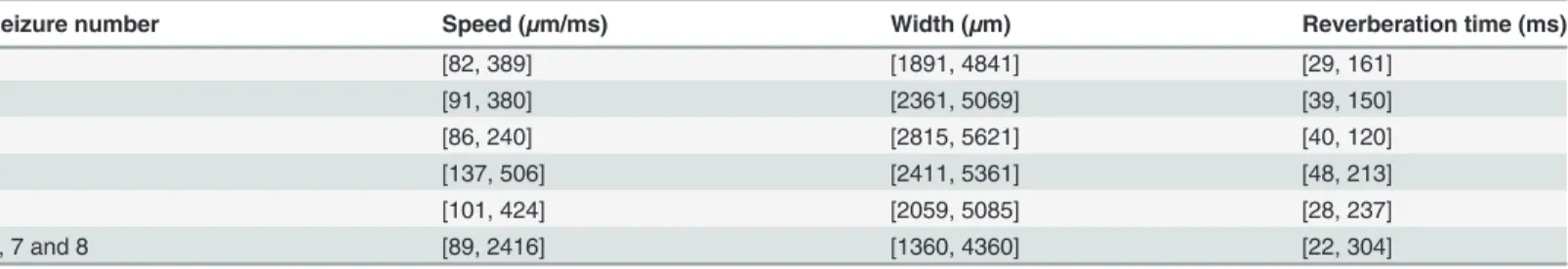
“reverberation time”(seeMethods). We show the results for the wave speeds and widths of all the analyzed waves inFig. 3, and the reverberation times histograms inFig. 4. These results are summarized for each seizure inTable 1where we show the mean speeds, mean widths, and mean reverberation times for the waves analyzed in each seizure. For each wave, we computed the mean values of the quantity of interest (speed, width, or reverberation time) over the differ-ent one-dimensional paths. The minimum/maximum values correspond to the minimum/ maximum obtained for the mean values of the quantity over the total of number of waves ana-lyzed for a given seizure. We note that for Patient 3 the data analysis was restricted due to the quality of the recordings (seeMethods).
For the three seizures of Patient 1 we observed consistent ranges of speed (≈80–380mm/ms), width (≈1900–5600mm), and reverberation times (≈30–150 ms). This suggests that similar, one-dimensional wave propagation patterns occur in the three seizures from this patient. For the two seizures of Patient 2, we also observed consistent ranges of speed (≈100–500mm/ms), width (≈2000–5300mm), and reverberation times (≈30–230 ms). Finally, for the three seizures of Pa-tient 3, we observed broader ranges of speed (≈90–2400mm/ms), width (≈1300–4300mms),
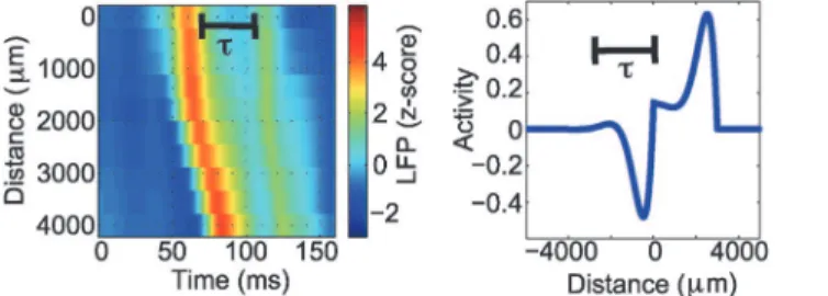
Figure 2. Illustration of two large amplitude waves followed by a reverberation of activity.The waves are plotted in one-dimensional space (vertical axis) as a function of time. The one-dimensional path extends across the two-dimensional microelectrode array (examples inFig. 1). This large amplitude wave is followed by a subsequent“reverberation”- a smaller amplitude wave (yellow or green in color). The horizontal black line indicates the reverberation time (τ). Warm (cool) colors indicate high (low) voltage values; scale bar at right.
Figure 3. Width versus speed of the traveling wave activity for the three patients.Each subplot shows the mean width and mean speed of each wave (red dots) together with a 90% confidence interval for both width and speed for each wave (vertical and horizontal blue lines). The confidence intervals are computed for each wave over the replicates of dimensional paths established for each wave (Fig. 1). In some cases, the existence of different one-dimensional paths produces a broad confidence interval for the estimate of the speed and width. In other cases, the existence of a unique one-one-dimensional path, or the estimation of the same quantity from the different one-dimensional paths, produces a narrow confidence interval.
doi:10.1371/journal.pcbi.1004065.g003
Figure 4. Reverberation time histograms of the seizure activity for the three patients.Each subplot shows the number of occurrences (or“counts”) of each reverberation time. For Seizures 1, 2 and 3 the maximum number of counts is between 60 to 70 ms; for Seizure 4, the values are broadly distributed between 100 and 200 ms; for Seizure 5 between 70 to 100 ms; and for Seizure 5, 6 and 7 between 40 to 70 ms.
and reverberation times (≈20–300 ms). These characterizations of thein vivowave dynamics provide information about the clinical observations, however an important question remains: what biological mechanisms support this traveling wave activity preceding seizure termination in the LFP? We propose to begin addressing this question in the next section through the inclusion of a mathematical model.
A mathematical model of traveling wave dynamics in LFP recordings
The mechanisms that produce organized neuronal population activity are extremely complex [58]. In an effort to characterize and understand the neuronal population activity observed in the clinical recordings preceding seizure termination, we implement here a relatively simple neural field model [59]. The biophysical basis for these types of models are understood by con-sidering the interaction of a finite number of synaptically coupled neurons. Many different for-mulations for neural fields exist [60], with implications for the interpretation of the model variables and parameters. These different mathematical formulations of neural field models can be broadly separated into two categories: voltage-based formulations, and activity-based formulations [59]. In a voltage-based model, the time scale of the dynamics is related to the membrane properties of the post-synaptic cells, while in an activity-based-model, the time scale of the dynamics is related to the synaptic decay [59]. We choose the latter formulation here. In its simplest form, the activity-based model is one of the most basic models to arise in mathematical neuroscience [61]. Beyond this simple form, activity-based models have been ex-tended to include additional features (e.g., absolute refractoriness [41,62]). In addition, the activity-based model is consistent with the notion that the LFP dynamics are dominated by the time scale of synaptic effects [10,63], and activity-based models have been proposed as more realistic than voltage-based models [64,65]. We note that most mathematical analysis of neural field models utilizes the voltage-based formulation [44,65,66]. In particular, in [67] the au-thors performed a complete analysis of the existence and stability of traveling wave solutions in the voltage-based formulation. To the best of our knowledge, a mathematical analysis of travel-ing wave existence and stability in an activity-based model with adaption has not beenperformed.
We now develop a one-dimensional model to describe important features of the neuronal population activity observedin vivo. The choice of a one-dimensional model is motivated by the observation that a majority of traveling waves observed in the LFP recordings travel in ap-proximately one-dimension, with features as described in the previous section. To simplify the model, we consider only a single population of excitatory neurons. In doing so, we will show that—in the mathematical model—inhibitory neurons are not required to mimic features of the observed LFP data immediately preceding seizure termination. To prevent the activity Table 1. Mean speeds, mean widths, and mean reverberation times for the waves analyzed in each seizure.
Seizure number Speed (μm/ms) Width (μm) Reverberation time (ms)
1 [82, 389] [1891, 4841] [29, 161]
2 [91, 380] [2361, 5069] [39, 150]
3 [86, 240] [2815, 5621] [40, 120]
4 [137, 506] [2411, 5361] [48, 213]
5 [101, 424] [2059, 5085] [28, 237]
6, 7 and 8 [89, 2416] [1360, 4360] [22, 304]
In this table, [a,b] indicate the minimum (a) and the maximum (b) of the corresponding measurement over the total number of waves analyzed for a given seizure.
from remaining in a permanent excited state, which will give rise to a front solution (see Meth-ods), we include an adaptation term that directly regulates the activity. This adaptation ac-counts for a natural process that will drive the population activity back to a rest state. From the mathematical point of view, adding this adaptation term permits traveling pulse solutions in the model consistent with key features of the clinical recordings. As we describe, using this rela-tively abstract and simple activity-based model with an adaptation term, we are able to replicate the reverberation observed in the LFP recordings.
The specific neural field model we employ is
utðx;tÞ ¼ auðx;tÞ þaH
1
2s
Z þ1
1
e jx ysjuðy;tÞdyþPðx;tÞ k
ab0qðx;tÞ
qtðx;tÞ ¼duðx;tÞ dqðx;tÞ;
ð1Þ
whereu(x,t) is the mean synaptic activity,q(x,t) is the adaptation, andP(x,t) is an external input, all evaluated at positionxand timet. In particular, we consider thatu(x,t) represents the activity of a cortical column with extent less than 20mm situated at positionxand timet. We interpretu(x,t), a dimensionless quantity, as the deviation from a baseline of activity. Therefore,u(x,t) = 0 represents a resting state of activity, and negative values represent a de-pression of resting activity [41]. We note that“negative activity”(i.e., a reduction in activity below the baseline rate) in one region reduces the input received in neighboring regions. In this formulation, we interpret the adaption term,q(x,t), as representing a local homeostatic regula-tion mechanism that evolves on a slower timescale thanu(x,t) and acts to maintain the activity near a target baseline. When the activityu(x,t) falls below the baseline value (i.e.,u(x,t)<0), the adaptionq(x,t) decreases which acts to increaseu(x,t). Conversely, when the activity in-creases above baseline (i.e.,u(x,t)>0), the adaptionq(x,t) increases and acts to decrease
u(x,t). We note that homeostatic regulation mechanisms act on a variety of timescales, includ-ing relatively short timescales (on the order of seconds) [68].His the Heaviside function, which becomes non-zero when the synaptic input exceeds a synaptic thresholdk:
Hðx kÞ ¼
1 ifxk
0 ifx<k:
(
We note that the adaptation term in (1) is located outside of the Heaviside function. In this phenomenological model with a simple adaptive scheme, the adaptation term acts as a local feedback mechanism to depress the synaptic drive. This model is motivated by the linear nega-tive feedback proposed in [44]. We note that, in voltage-based models, different formulations for adaption exist; these include negative feedback both inside the threshold function [44,51, 69] and outside of the threshold function [49,53]. We show inS1 Textof Supporting Informa-tion that the model (1) updated to include the adapInforma-tion term inside of the Heaviside funcInforma-tion does not produce damped oscillations; instead, the traveling wave solution returns monotoni-cally to rest after excitation. This monotonic evolution is inconsistent with the reverberation observed in the LFP data of interest here (examples inFig. 2).
There are 5 parameters in the model (1). Each possesses a biological interpretation:αis the decay rate parameter for the synaptic activity term,δis the decay rate parameter for the adapta-tion term,sis the spatial rate of decay of connectivity,kis the synaptic input threshold, andβ0
accounts for the strength of the adaptation term on the synaptic dynamics. For simplicity we setβ=αβ0. Both time and space units were scaled to represent milliseconds and microns,
Our goal is to identify the parameter configurations that support traveling waves in this model consistent with the observed LFP activity. In particular, we are interested in solutions that support only one extremum of high amplitude activity, so called pulses, as these have been characterized using the LFP data. To that end, we first determine under what parameter config-urations traveling waves of high amplitude activity exist in the model. To do so, we rewrite the equations in a moving coordinate framez=x−ct; this frame is moving with a constant speedc. By identifying the stationary solutions of this system, we determine solutions that move with a constant speedc, and a constant widthw, without changing their shape: so called traveling waves. Depending on the model parameters, we find that the linearization of the associated system in the moving coordinate frame consists of either purely real or complex eigenvalues. The explicit traveling wave solutions for both the real and imaginary case are now considered. We state the solutions here; detailed analysis may be found in Methods.
Traveling Wave Solution: Real Eigenvalues Case
We begin by considering the case in which the eigenvalues of the associated linear system of (1) are purely real. This occurs whenb<ða dÞ2
4d (seeMethods), and the traveling wave solution
of the activity of widthwand speedcin the moving coordinate framez=x–ctis:
uðzÞ ¼
0 ifzw
a
dðaþbÞðlþ l Þðl e
lþðz wÞðd cl
þÞ lþe
l ðz wÞðd cl Þ þdðl
þ l ÞÞ
if0<z<w a
dðaþbÞðlþ l Þðl ðe
wlþ 1
Þðd clþÞelþzþl
þð1 e
wl
Þðd cl Þel zÞ
ifz0;
8
> > > > > > > > > <
> > > > > > > > > :
wherel¼1
2cðaþd
ffiffiffiffiffiffiffiffiffiffiffiffiffiffiffiffiffiffiffiffiffiffiffiffiffiffiffiffiffiffiffiffiffiffiffiffiffiffiffiffiffiffi ðaþdÞ2
4dðaþbÞ
q
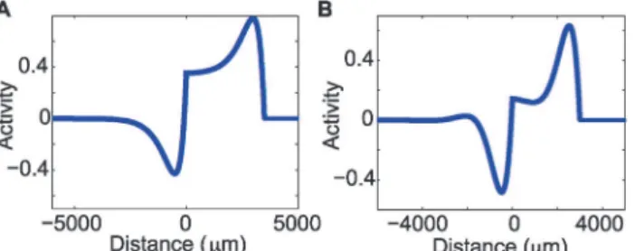
Þ. In this traveling wave solution (Fig. 5a), a pulse is followed by a depression of activity; this depression is due to the adaptation term. The activity then returns to a rest state after this depression in a monotonic fashion.
Figure 5. Analytic solution for the traveling pulse in the real and complex eigenvalue case. (a)The onset of the pulse consists of a rapid increase in activity, followed by a rapid decrease due to adaptation, and then a monotonic return to rest (zero activity). In this figureα= 20/s,δ= 2/s,β= 1.5,σ= 200μm,c= 180μm/ ms andw= 3500μm.(b)In the complex eigenvalue case there is a pulse followed by a depression of activity due to the adaptation term. Unlike the solution in the real eigenvalue case, damped oscillations follow this depression as activity returns to the rest state. In this figureα= 20/s,δ= 2/s,β= 4.6,σ= 160μm,c= 250μm/ ms andw= 3000μm.
Traveling Wave Solution: Complex Eigenvalues Case
We now consider the case in whichb>ða dÞ2
4d . In this scenario, the linearization of the
associat-ed system of (1) contains imaginary eigenvalues, and the traveling wave solution of the activity of widthwand speedcin the moving coordinate framez=x–ctis:
uðzÞ ¼
0 ifzw
a aþbþ
2a ffiffiffi
b
p
eð Þa2þcd ðz wÞ ffiffiffiffiffiffiffiffiffiffiffiffiffiffiffiffiffiffiffiffiffiffiffiffiffiffiffiffiffiffiffiffiffiffiffiffiffiffiffiffiffiffiffiffiffiffiffiffi ðaþbÞð4bd ðd aÞ2Þ
q sin
ffiffiffiffiffiffiffiffiffiffiffiffiffiffiffiffiffiffiffiffiffiffiffiffiffiffiffiffiffiffi
4db ða dÞ2
q
2c zþj1
0
@
1
A if0<z<w
2a ffiffiffi
b
p
eð Þa2þcdðzÞ ffiffiffiffiffiffiffiffiffiffiffiffiffiffiffiffiffiffiffiffiffiffiffiffiffiffiffiffiffiffiffiffiffiffiffiffiffiffiffiffiffiffiffiffiffiffiffiffi ðaþbÞð4bd ðd aÞ2Þ
q Dcos
ffiffiffiffiffiffiffiffiffiffiffiffiffiffiffiffiffiffiffiffiffiffiffiffiffiffiffiffiffiffi
4db ða dÞ2
q
2c zþj2
0
@
1
A ifz0;
8 > > > > > > > > > > > < > > > > > > > > > > > : where D¼ ffiffiffiffiffiffiffiffiffiffiffiffiffiffiffiffiffiffiffiffiffiffiffiffiffiffiffiffiffiffiffiffiffiffiffiffiffiffiffiffiffiffiffiffiffiffiffiffiffiffiffiffiffiffiffiffiffiffiffiffiffiffiffiffiffiffiffiffiffiffiffiffiffiffiffiffiffiffiffiffiffiffiffiffiffi
1 2e wðaþ2cdÞcos
ffiffiffiffiffiffiffiffiffiffiffiffiffiffiffiffiffiffi
4db ða dÞ2
p
2c w
þe wðaþd
cÞ
s
j1¼tan 1
ðA1 A2Þ þ
p ifA1 <0 0 ifA1 >0
;j2¼tan 1 A3
A4
þ
p ifA4 <0
0 ifA4 >0
( (
A1¼ ð2bþa dÞsin
ffiffiffiffiffiffiffiffiffiffiffiffiffiffiffiffiffiffi
4db ða dÞ2 p
2c w
ffiffiffiffiffiffiffiffiffiffiffiffiffiffiffiffiffiffiffiffiffiffiffiffiffiffiffiffiffiffi
4db ðd aÞ2
q
cos
ffiffiffiffiffiffiffiffiffiffiffiffiffiffiffiffiffiffi
4db ða dÞ2 p
2c w
A2¼ ð2bþa dÞcos
ffiffiffiffiffiffiffiffiffiffiffiffiffiffiffiffiffiffi
4db ða dÞ2 p
2c w
ffiffiffiffiffiffiffiffiffiffiffiffiffiffiffiffiffiffiffiffiffiffiffiffiffiffiffiffiffiffi
4db ðd aÞ2
q
sin
ffiffiffiffiffiffiffiffiffiffiffiffiffiffiffiffiffiffi
4db ða dÞ2 p
2c w
A3¼
ffiffiffiffiffiffiffiffiffiffiffiffiffiffiffiffiffiffiffiffiffiffiffiffiffiffiffiffiffiffi
4db ða dÞ2
q
þe a2þcdwA1
A4¼ ð2bþa dÞ þe aþd
2cwA2:
The solution for the complex eigenvalue case results in a pulse followed by a depression of ac-tivity due to the adaptation term. Unlike the solution in the real eigenvalue case, damped oscil-lations follow this depression as activity returns to the rest state (example inFig. 5b). We note that the damped oscillations are dominated by a single positive deviation above rest, following the depression. This positive deviation is similar to the reverberation of activity following the traveling wave observed in the LFP (Fig. 2). We note (seeS1 Textof the Supporting Informa-tion) that a different model with the adaption term included inside of the Heaviside function in (1) is unable to reproduce the damped oscillations observed in the LFP data.
Solution curves from matching conditions
The interactions of neighboring cells affect the activity at a pointx. In the presence of a pulse of high activity, such interactions reach the synaptic thresholdkat exactly two points, sayx0
andx1. The distance betweenx0andx1is the width of the wavewand the pointsxcontained
within (x0,x1) satisfy 1 2s
Z þ1
1
e jx ysjuðy;tÞdy>k. At bothx
0andx1, this inequality becomes an
equality, i.e., the interaction term equals the synaptic thresholdk. Equating the interaction terms atx0andx1defines the matching conditions. To simplify the analysis, and without loss
of generality, we considerx0= 0 andx1=w. By fixing the parametersα,δ,sandβand by
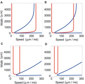
c-wplane, the intersection of these curves determines the existence of traveling wave solutions to the model (1). Depending on the choice of parameters, there may exist no traveling waves, one traveling wave, or two traveling waves (examples inFig. 6). We find that, for a solution with two traveling waves, one of the waves is slow and narrow, and the other wave is fast and wide (Fig. 6b).
If we consider instead fixed values ofc,w,α,δand solve the matching conditions, we obtain a solution curve in theβ-splane that determines, if they exist, parametersβandsfor which we have
a pulse with given speedcand widthw. Moreover, by consideringk¼ 1 2s
Z þ1
1
e jsyjuðy;tÞdyor
k¼ 1 2s
Z þ1
1
e jw ysjuðy;tÞdy, we can solve for the thresholdkcorresponding to the choice ofsand
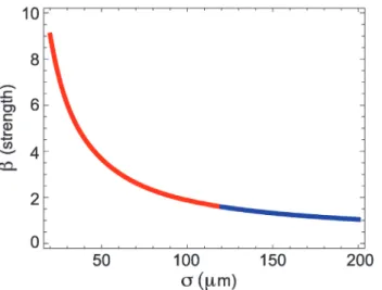
β(for more details, seeMethods). To illustrate the application of the matching conditions, we con-sider one typical traveling wave observed in the LFP recording with speedc= 179mm/ms and widthw= 3500mm. For this example, we fixα= 20/s andδ= 2/s, and find a solution curve for the wave of the specified speed and width as a function of the two parametersβands. The solution curve consists of both real and imaginary parts (blue and red, respectively, inFig. 7), corresponding to the real and complex eigenvalue cases of traveling wave solutions of the model (1). We note that all of the points along the solution curve satisfy the constraints of speed and width; additional con-straints are required to select a single point on this curve.
Figure 6. Width versus speed in the mathematical model for different values of the thresholdk.The four subplots show the existence of waves given by the points of intersection of the matching conditions. The blue and red curves indicate the matching conditions at the points 0 andw, respectively. We fixα= 25/s,δ= 2.5/s,σ= 120μm,β= 2.05, and by varyingkwe obtain the existence of no waves (d), one wave (a,c), or two waves (b).(a)The two curves intersect at a single point to specify a wave with speed 30μm/ms and width 112μm.(b)The two curves intersect at two points, resulting in a wave with speed 33μm/ms and width 164μm, and a wave with speed 220μm/ms and width 2679μm/ms.(c)The two curves intersect at a single point to specify a wave with speed 71μm/ms and width 350μm.(d)The two curves do not intersect, and therefore no wave solutions exist.
The period of the reverberation fixes the model parameterβ
The mathematical model (1) contains five free parameters:α,δ,s,βandk. In the previous sec-tion, we began restricting these parameters by establishing relationships between parameters that support traveling wave solutions. In particular, by fixing the time scalesαandδ, together with a choice of speedcand widthwdeduced directly from the LFP data and hence constrained by the clinical observations, we may solve for the remaining parametersβ,s, andk. The match-ing conditions establish a relationship betweensandβ(example inFig. 7), and by choosingβ
andswe can solve for the correspondingk, as described in the previous section. We now pro-ceed to use the“reverberation”observed in the clinical data (examples inFig. 2) to estimate the parameterβfor each wave. In doing so, we will have used the clinical data and biophysical intu-ition to constrain further the model parameters.
Visual analysis of thein vivoLFP data shows that high amplitude pulses are followed by a reverberation, i.e., a secondary, smaller amplitude increase in activity (for more details, see Methods). Due to the nature of the traveling wave solutions, this feature is only present in the complex eigenvalue solution, i.e., when damped oscillations follow the pulse of high amplitude activity (example inFig. 5b); we propose that the damped oscillations following the main pulse of the traveling wave mimic the reverberations observed in the LFP recordings. Hence, we re-strict the following analysis to the complex eigenvalue case. We use the reverberation times es-timated from the LFP data to fix the parameterβfor each wave; we label these estimates
βempirical. To do so, we set the periodic portion of the complex eigenvalue solution to possess a period consistent with the observed reverberation: given a reverberation timet(example in Fig. 8), thenbempirical¼ðd a4dÞ2þ
4p2
dt2(seeMethods). In this way we constrain the model to
repli-cate the period of the secondary bump (i.e., reverberation) present in the data (Fig. 8). Having done so, the model parametersβ,s, andkare now directly determined for each observed LFP wave.
Figure 7. Solution curve in theσ-βplane obtained from the matching conditions in the mathematical model.We show the complex eigenvalues case (red) and the real eigenvalues case (blue). The parameters arec= 179μm/ms,w= 3500μm,α= 20/s,δ= 2/s. The curve shows pairs ofβandσfor which a wave of speedcand widthwexist. By using the matching conditions we can determine the parameterk
Restriction of the ratio between activity and adaptation timescales
In the previous sections, we used features of the traveling wave data (the speed, width, and re-verberation time) to constrain three model parameters:β,s, andk. Two model parameters -α
andδ- remain unconstrained. We now consider how different choices of the model timescales
αandδimpact the existence of traveling wave solutions consistent with the LFP data. To do so we focus on two different orders of magnitude between the timescales and considerα/δ= 10 andα/δ= 100. These equations and the model (1) are consistent with the notion that adapta-tion (with timescale determined byδ) occurs more slowly than synaptic activity (with timescale determined byα). Moreover, once we fix the ratioδ=α/10 (orδ=α/100) we can estimatec,w
andβfrom the clinical recordings and obtainsandkfrom the matching conditions. Therefore, only a single free parameter remains:α. The rest of the parameters are constrained by either the clinical data or the matching conditions of the mathematical model.
To characterize the impact of different choices ofα, and the ratioα/δ, we fix both parame-ters in the model and determine whether the model supports wave activity consistent with the observed data and physical assumptions in the model. We therefore exclude solutions in which the matching conditions specify a connectivity extent (s) of less than 20mm; these solutions are too small and inconsistent with the notion that the model (1) represents the activityuof coupled cortical columns. InFig. 9we show the percentage of waves for each seizure with a physically reasonable value ofs>20mm for different choices ofαand ratiosα/δ. For all of the seizures from all three patients, we find that the model successfully reproduces the observed waves, and remains physically reasonable (s>20mm), for intermediate values ofαandδ=
α/10 (Fig. 9a–c). For a smaller value ofδ=α/100, the model performs more poorly; i.e., the model produces more physically unreasonable solutions (Fig. 9d–f). We note that, for Patient 3, the waves are more difficult to reproduce compared to the other two patients. We conclude that the model best replicates the observed traveling waves in the LFP data preceding seizure termination whenδ=α/10. At this ratio, a broad range of values inαexist that support physically reasonable solutions.
Relationship between adaptation timescale and model parametersβ0,kandσ
With the ratioδ=α/10 now fixed, we proceed to analyze the relationship betweenαand three other model parameters:β0,kands. We recall thatβ0is the strength of the adaptation and
β0=β/α. InFig. 10andTable 2we summarize the results of these relationships for the three
pa-tients. Based on the analysis shown inFig. 9, we examineαbetween 12/s and 75/s, for which the model tends to successfully reproduce the observed waves for all three patients. In particu-lar, above 90% of the analyzed waves are replicated in this range ofαfor all seizures. We find Figure 8. Illustration of the parameterβin the mathematical model estimated from the LFP data.Given a wave with a reverberation time ofτ= 45 ms (left figure) and the approximate period of the complex eigenvalue pulse solution (right figure) we obtain a correspondingbempirical¼1
dð 4p2
t2 þð
for Patients 1 and 2 that the values of the parametersβ0,s, andktend to remain consistent from seizure to seizure as a function ofα. We also note that, forαsufficiently large (i.e.,α>
25/s), the variability of these estimates across the traveling wave events is relatively small (Fig. 10). Moreover, the parameter estimates produce similar values, both within each patient and between the two patients (Fig. 10andTable 2). For Patient 3, we find that the parameter estimates exhibit more dependence onαand are more variable. However, even these estimates remain consistent with the other patients and seizures.
We note that, for large values ofα, the estimates ofβ0tend to converge to similar values
(Fig. 10). To understand this, we use the explicit formula forβempiricalin terms of the reverbera-tion time:bempirical¼ðd aÞ2
4d þ
4p2
t2d¼bmaxþ 4p2
t2d. Substitutingδ=α/10 we then obtain
bempirical¼81 40aþ
40p2
t2a. This implies that smaller values ofαand the reverberationthave bigger
impacts on the value ofβempirical. Due to the small values oftobtained from Patient 3 (see Table 2), larger variability in the values ofβ0appears at smallα(Fig. 10). Moreover, since
b0 ¼
bempirical
a ¼
81 40þ
40p2
t2a2, we obtain that asαincreasesβ0converges to 81
40(this limit is determined
by the specific choiceδ=α/10), explaining the convergence seen inFig. 10to a specific value of
β0. Similar trends appear in the other parameter estimates (Fig. 10) and the implicit equations
of the matching conditions determine these trends. To illustrate, we observe inFig. 7that asβ
increases (andβ0decreases),sdecreases, explaining the convergence ofsasαincreases
(Fig. 10, middle row).
Figure 9. The percentage of waves from each seizure for which it is possible to find a physically reasonable solution (σ>20μm) as the parameter
αis varied.In the first row we fixδ=α/10, a difference of one order of magnitude between the timescales. In the second row we fixδ=α/100.(a)We note that for the three seizures of Patient 1 a value ofαbetween 15/s and 53/s produces physically reasonable solutions for all analyzed waves.(b)For the two seizures of Patient 2 a value of between 15/s and 75/s produces physically reasonable solutions for 90% of the analyzed waves.(c)For all seizures of Patient 3, givenαbetween 25/s and 150/s produces physically reasonable solutions for 90% of the analyzed waves.(d-f)At the ratioδ=α/100, the model solutions tend to be unphysical (i.e.,σbecomes too small) forα>12/s. This analysis suggest that the model best replicates the observed LFP data whenδ= α/10.
Figure 10. Relationships between the timescale parameter and other model parameters suggest similar features across all patients and seizures. The subplots show the relationship betweenαandβ0(row 1),αandσ(row 2), andαandk(row 3). Patient 1 is in column 1, Patient 2 in column 2, and Patient 3 in column 3. For Patient 1,β0is between 2 and 3,σis between 40 and 250μm/ms, andkis between 0.15 and 0.17. For Patient 2,β0is between 2 and 3,σis between 40 and 1000μm/ms, andkis between 0.15 and 0.17. For Patient 3, for 25/s<α<75/s,β0is between 2 and 10:σis between 60 to 4000μm/ms andkis between 0.1 to 0.2.
doi:10.1371/journal.pcbi.1004065.g010
Table 2. Range of parameters supporting wave propagation,fixingδ=α/10.
Seizure number α(1/s) β0(strength) σ(μm) k(synaptic threshold)
1 15–53 2–2.5 50–250 0.15–0.17
2 15–58 2–2.3 40–180 0.16–0.17
3 15–55 2–2.3 40–130 0.15–0.17
4 15–78 2–2.2 40–600 0.16–0.18
5 15–150 2–2.3 20–300 0.16–0.17
6,7, and 8 25–150 2–4 60–4000 0.12–0.2
Seizures 1, 2 and 3 correspond to Patient, 1, Seizures 4 and 5 correspond to Patient 2 and Seizures 6, 7 and 8 correspond to Patient 3. We note that consistent parameter ranges forβ0,σandkappear in seizures of the same patient. We also note in comparison with Patient 1, the parameters forσ include larger values for Patient 2 and Patient 3.
Numerical simulations of the model produce one-dimensional waves
consistent with the LFP data
As a final illustration of the suitability of the model, we consider an example numerical simula-tion of the model (1) (seeMethods). To do so, we choose a particular wave from the LFP data of Seizure 1, estimatecandwdirectly from the data, and fixα= 7.5/s, as for this value ofα
non-trivial parameters from both the real and complex eigenvalue solutions can be obtained from the matching conditions. Following an initial stimulus (5 ms initial input at position 0mm) the model produces a traveling pulse that is followed by a smaller amplitude reverbera-tion. A comparison of a wave from the clinical recordings with the real and complex eigenval-ues case is shown inFig. 11. We note that both simulations accurately replicate features of the observed LFP wave (namely, the speed and width), but that the complex eigenvalue case solu-tion also produces a secondary bump of activity consistent with the reverberasolu-tion in the ob-served LFP wave. We also note that, in the model, the activity decreases below 0 between the mean crest of the traveling wave and the subsequent reverberation of activity inFig. 11(c). A decrease in activity also appears in thein vivodata between the crest of the traveling wave and the reverberation (example inFig. 11(a)); however, this decrease is smaller in magnitude than that produced in the model. An updated model that includes inhibition helps reduce this dis-crepancy, as illustrated in the next subsection.
Numerical simulations of a model with inhibition produce additional
consistency with the LFP data
The original model formulation (1) is analytically tractable and capable of reproducing impor-tant features of the observed traveling wave dynamics. However, as expected, this relatively simple model exhibits some inconsistencies with thein vivodata, for example the large negativ-ity following the traveling wave crest.
Increasing the complexity of the model through the addition of more biological features may help reduce these inconsistencies. To that end, we consider an updated model that in-cludes an inhibitory population. In particular, we implement the following system:
utðx;tÞ ¼ aeuðx;tÞ þaeHðgeeuðxÞ gievðxÞ þPðx;tÞ keÞ ab0qðx;tÞ
qtðx;tÞ ¼duðx;tÞ dqðx;tÞ
vtðx;tÞ ¼ aivðx;tÞ þaiHðgeiuðxÞ giivðxÞ þQðx;tÞ kiÞ;
ð2Þ
Figure 11. The simulated and observed data are consistent. (a)A wave from Seizure 1 with speedc= 179μm/ms and widthw= 3535μm.
(b)Parameters obtained from the real eigenvalue solution,α= 7.5/s,β0= 2.9,σ= 100μm. The wave has a speed ofc= 178μm/ms and widthw= 3698μm. (c)Parameters obtained from the complex eigenvalue solution,α= 7.5/s,β0= 2.5,σ= 160μm. The wave has a speed ofc= 178μm/ms and widthw= 3698 μm. The positive activity reverberation in yellow is visible following the main wave in red and blue. The color scale is chosen to allow visualization of the smaller amplitude reverberation.
whereu(x,t) is the mean synaptic activity of the excitatory population,v(x,t) is the mean syn-aptic activity of the inhibitory population,q(x,t) is the adaptation term in the excitatory popu-lation, andP(x,t) andQ(x,t) are external inputs to the excitatory and inhibitory populations, respectively. The convolutions account for the spatial extent of the synaptic connectivities,
gjkwðxÞ ¼gjk
1
2s
jk Z þ1
1
e j x yj sjk
wðy;tÞdy;
wherej= {e,i},k= {e,i}, andg
jk¼ f0;1g.His the Heaviside function, which becomes
non-zero when the total input exceeds the thresholdkj.
To characterize the behavior of this model, we perform numerical simulations. We set the parameters to match the wave speed and width used for the original model (1) inFig. 5b, and fixαi= 2.5/s,ki= 1,sei= 20mm,sie= 20mm, andsii= 0. We first consider the casegei¼0,
gie¼0andgii¼0so that the excitatory and inhibitory populations do not interact. The
result-ing wave profile (Fig. 12a) reveals a large amplitude pulse, followed by a deep depression of ac-tivity, and then a smaller amplitude reverberation, as expected for the original model
formulation (1). Then, using the same parameter settings, we activate interactions between the excitatory and inhibitory populations (g
ei¼1,gie¼1,gii¼1). The resulting wave profile
(Fig. 12b,c) exhibits qualitative differences from those in the original model; by including inhi-bition, the wave profile becomes smoother and thinner, and the depression of activity following the large amplitude pulse is shallower. These results suggest that a neural field model with ad-aptation and inhibition produces wave profiles with additional features consistent with thein vivodata, including a smoother wave profile and a shallower depression of activity following the main pulse. We conclude that the original model (1), even in the absence of inhibition, sup-ports wave propagation as observed in the clinical recordings. However, incorporating addi-tional biological features in the model - such as inhibition - may improve fidelity with the clinical data.
Discussion
In this paper, we considered invasive local field potential (LFP) recordings from a population of human patients during seizures. We showed that, in the late stages of seizures, spatiotempo-ral patterns of activity propagate across a small patch of cortex. These patterns can be well ap-proximated as one-dimensional plane waves, and we characterized important features of these waves (i.e., the speeds and widths). We found traveling wave speeds of≈80–380mm/ms, con-sistent with the propagating velocity of a pulse when GABAergic local inhibition is blocked Figure 12. A model that includes inhibition produces additional features consistent with thein vivodata. (a)Wave profile obtained from the original model without inhibition ( g
ei¼0, gie¼0 and gii¼0). The parameters used areαe= 25/s,δ= 2.5/s,β= 5,σee= 52μm andke= 0.14. The depression of activity reaches approximately -0.5 and is followed by a small reverberation of activity.(b)Wave profile obtained in the updated model that includes inhibition ( g
ei¼1, gie¼1, gii¼1). The wave has a smoother profile and the depression of activity does not reach -0.5. The width of the wave is reduced to around
(e.g., 60–90mm/ms in [70], 70mm/ms in [71], 130–190mm/ms in [25], and 120–150mm/ms in [72]). In addition, we examined the features of small amplitude“reverberations”in the voltage activity following each wave.
To further characterize the observed LFP waves, we implemented a relatively simple neural field model consisting of an excitatory population of cells with adaptation. This abstract mathe-matical model is flexible enough to replicate important features of wave propagation near sei-zure termination for the population of patients and seisei-zures. Moreover, the relative simplicity of the model permits analytic solutions; we showed here, for the first time, that traveling wave solutions exist and are stable in this activity-based model formulation with adaptation. In addi-tion, the model parameters permit biophysical interpretation (e.g., as the extent of synaptic connectivity). By combining analytic model solutions with features of the observed waves -such as the speed and width - we estimated parameters in the model. The estimated parameters included the timescales of activity and adaptation, and the spatial extent of the connectivity. We find that the timescale of the model consistent with the observed LFP data is biologically reasonable: the adaption is an order of magnitude slower than the activity. Measures of synap-tic connectivity in a local neighborhood of corsynap-tical tissue have been reported to range from 40mm to 2 mm [12,41,63,73–75]. For the deduced range of parameters obtained in this study, we find that the extent of connectivity,s, for Patients 1 and 2 coincides with this estab-lished range. For Patient 3, we obtain connectivities between 60mm to 4 mm, which is larger, but not wholly inconsistent with existing estimates. We find for all three patients that the pa-rameterβ0, which is the strength of the adaptation, is between 2 and 4; and the parameter k,
which accounts for the synaptic threshold, is between 0.12 and 0.2. The variability in the esti-mates ofs,β0andkmay reflect changing biophysical features during seizure (e.g., progressive
changes in synaptic efficacy or changes in the extracellular environment) as well as the variabil-ity inherent in measuring a noisy biological system. We also note that for the three patients, as the timescale of the activity increases, the extent of the connectivity decreases (Fig. 10) suggest-ing that faster activities (largeα) require less distant connectivity. Finally, we note that the pa-rameter estimates are consistent both within individual patients, and across the population of patients and seizures. We conclude from these results the following hypothesis: plane waves observedin vivolate in human seizure can be supported in a relatively simple mathematical model without inhibition, consistent within vitroslice and theoretical work (e.g., [25,36,70–
72,76–78]). However, we note that inclusion of inhibition may improve features of the model (e.g., may better mimic aspects of the wave profile, seeFig. 12andS2 Textin Supporting Infor-mation for additional illustrations).
The analysis and modeling focused on an interval preceding seizure termination, in which the data have transitioned to large amplitude spike-and-wave (or spike-and-polywave) oscilla-tions. A goal of this modeling study was to simulate some of the spatiotemporal aspects of this wave activity. Animal studies suggest the mechanisms that support this spike-and-wave activity are complex. Some studies have suggested that the“wave”component of the spike-and-wave oscillation reflects inhibitory GABAergic processes [79–81]. However, other animal studies instead propose that slow intrinsic currents (e.g., a calcium-activated potassium current) support the“wave”component of the spike-and-wave oscillation [82–87], andin vitro
inhibitory mechanisms may engage in the generation of the depolarizing component of spike-and-wave oscillation.
Here we have implemented a mathematical model with a tight focus on one aspect of the late seizure interval: the (approximately) one-dimensional traveling waves that appear in spike-and-wave oscillations near seizure termination. In doing so, we have presented a modeling for-mulation more consistent with the proposed intrinsic current mechanisms of spike-and-wave oscillations. Nevertheless, we suspect that inhibition plays a fundamental role in seizure, for ex-ample at seizure onset [90,91] when fast-spiking interneurons are highly active. We expect that the addition of more biophysical features to the model (including inhibition) will permit a better match to thein vivoLFP data (seeFig. 12andS2 Textof Supporting Information), at the cost of increased model complexity and reduced analytic tractability.
In this work we implemented a relatively simple one-dimensional neural population model, consisting of a synaptic activity variable and an adaptation variable. The simplicity of the model allows rigorous mathematical analysis, although the biophysical mechanisms re-main relatively abstract. The validity of the model is based on the reproduction of wave fea-tures present near seizure termination, and parameter estimates consistent with known physiology (i.e., estimates of synaptic connectivity and difference in timescales). The purpose of this model is not to capture the detailed biophysical mechanisms of seizure, as in more re-alistic computational models [92,93]. However, we may use the mathematical model to make the following prediction: the traveling waves near seizure termination represent relatively
“simple”brain phenomena. Consistent with this notion, we hypothesize that the diversity of complex components that support normal cortical function (e.g., the diversity of inhibitory neuronal populations [94,95]) have shut down, and allowed these simple dynamics to domi-nate. Restoration of this diversity and complexity (e.g., activation of silenced inhibitory neu-ronal populations) would then help disrupt these pathologically organized and simple traveling waves.
To further validate the model results,in vitroexperiments that reproduce important features of the humanin vivodata (e.g., the spectrographic properties [90,96]) would allow detailed pharmacological exploration of the proposed biophysical mechanism of this model. In particu-lar, the more abstract model parameters (likeβ0, the strength of the adaptation) may be better understood in terms of specific neuronal mechanisms through experiments in controlled bio-logical systems. These experiments may in turn motivate future work developing more biologi-cally detailed models to provide additional insight into the spatiotemporal dynamics of seizure activity. One important future modeling direction is the further analysis and inclusion of inhib-itory populations in this activity-based formulation. Such inclusions may further illuminate the mechanisms of wave propagation, and might help to explain differences in waves seen during the initial and terminal stages of human seizure.
Materials and Methods
Ethics Statement
All patients were enrolled after informed consent was obtained and approval was granted for these studies by local Institutional Review Boards.
Data Analysis
For each patient and seizure, we analyzed a subset of the diverse spatiotemporal patterns ob-served approaching seizure termination. We focus here on the analysis of one-dimensional plane waves of activity, which were the most common type of wave we observed in Patients 1 and 2 (Seizure 1, 36 out of 40 waves; Seizure 2, 36 out of 41; Seizure 3, 39 out of 59; Seizure 4, 26 out of 33; Seizure 5, 35 out of 52). Upon visual inspection, the excluded waves exhibited dif-ferent spatiotemporal patterns, including disorganized waves of high activity, and
two-dimensional patterns, such as waves that initiated at the center of the microelectrode array, and spiral waves. Again, we focus here only on the one-dimensional plane waves and estimates of the model parameters from these waves. For Patient 3, we focused on a contiguous half (2 mm by 4 mm) subsection of the entire (4 mm by 4 mm) microelectrode array. For this patient, we were able to detect waves moving closer to the horizontal direction (from−45° to 45° and from 135° to 225°). Having selected these one-dimensional waves from the three patients, all waves were analyzed using the same set of data analysis algorithms described below. Components of these data may be made available by request to the corresponding author.
The purposes of the data analysis were: i) To obtain a time interval for the propagation of each planar wave; ii) To obtain the direction of wave propagation; iii) To obtain the different one-dimensional paths through the two-dimensional microelectrode array for a given direc-tion; iv) To obtain the speed, width, and reverberation time along each one-dimensional path; and v) To obtain the mean speed, mean width and mean reverberation time for each wave across different paths. To determine the time interval for the propagation of each planar wave, we computed the gradient of the LFP activity at each moment in time. The gradient assigns to each spatial location a vector specifying the direction and magnitude of maximal increase in ac-tivity (Fig. 13a). To compute the gradient, we analyzed voltage differences between adjacent electrodes. A histogram of the angles of the gradient at each position, weighted by the magni-tude of the gradient, was then constructed for each moment in time (Fig. 13b). We labelt0the
Figure 13. Example of LFP data analysis procedure. (a)Example of a vector field before a wave enters the microelectrode array. For each of the interior electrodes, an angle is assigned according to the gradient.(b)Example weighted angle distribution for the time interval (t0−14 ms,t0+ 100 ms) for a single wave during a seizure. In this example,tinitial= 14 ms andtfinal= 100 ms. The peak of the distribution occurs at angleθ0.(c)Illustration of the different computed quantities:θ0is the peak of the distribution;θ1=θ0+180c, wherec=1 (depending on the value ofθ0);tinitialis the time at which the phase interval
(θ0-20,θ0+20) acquires non-zero counts;t0is the time at which the LFP z-scored signal at the center of the microelectrode array exceeds a threshold; and
time at which the LFP z-scored signal at the center of the microelectrode array exceeded a threshold of 2.5. We then determined the peak of the unimodal angle distribution at timet0,
which we labeledy0. We considered angles betweeny0−20 andy0+20 degrees and analyzed the
proportion of angles within the interval (y0−20,y0+20), forward and backwards in time
start-ing att0. The timetinitialdenotes the first time at which the number of counts in the angular
in-terval becomes non-zero. The timetfinalis the last time at which counts appear in the angular
interval. In this way, each wave is assigned a time interval (tinitial,tfinal) for which angles appear
in the interval (y0−20,y0+20). In this time interval, the weighted histograms of the angles
showed a clear organization of the gradient directions and appearance of two peaks in the his-togram distributions (Fig. 13b). These two peaks account for the preferred angle before the wave enters the microelectrode array and after the wave exits the microelectrode array. To de-termine the direction of each wave we focused on the first peak (Fig. 13b). This peak typically occurs in the time interval (tinitial,t0). In addition, we visually inspected each peak and verified
that the associated angle accurately described the direction of propagation for each wave. The notions oft0,tinitial,tfinalandy0are illustrated inFig. 13c.
Having determined the angle at which LFP activity propagated, we then constructed one-dimensional paths spanning the microelectrode array. Each path consisted of 10 adjacent elec-trodes and ran parallel to the direction of the observed wave. Along each such path we deter-mined the speed and width of the wave. For each path, we deterdeter-mined the time at which the activity at each electrode exceeded a threshold of one standard deviation above the mean LFP computed for the entire duration of seizure termination investigated. In this way, every elec-trode along a path was assigned a time of wave onset, which was used to compute the speed. We used all possible combinations of the 10 electrodes along each one-dimensional path to compute the speed, resulting in a total of 45 estimates of speed. To mitigate the impact of outli-ers, the speed for each one-dimensional path was then calculated as the median of the 45 speed estimates. We then estimated the speed for each wave as the mean speed among the different one-dimensional paths. Depending on the direction of the wave, from the 10 electrodes that form a one-dimensional path, there is one electrode at which the large amplitude activity of the wave reaches last, and we label this the“last electrode”(example inFig. 14). To measure the wave width, for each one-dimensional path we computed the time at which the activity at the last electrode exceeded a threshold of 2.5 of the LFP z-scored signal. At that instant in time, the
activity of the other electrodes along the path was also determined. The location at which the activity transitioned from above the threshold (of 2.5 of the LFP z-scored signal) to below the threshold was determined. The spatial extent from the last electrode to this transition point on the one-dimensional path defined the width of the wave. An illustration of the wave width determination is shown inFig. 14. We note that if no electrode along the one-dimensional path transitioned to below the threshold, then the wave covered the entire spatial extent of the path, and the width of the wave indicates a lower bound. For each wave, the width refers to the mean widths obtained from all one-dimensional paths. To obtain the reverberation time we first de-termined the time at which the large amplitude wave of activity fell below a threshold of 0.5 of the LFP z-scored signal; we consider this time as the“end”of the primary traveling wave. Start-ing from this time point, we then determined the time for the activity to first exceed a reverber-ation threshold, defined as 0.5 of the LFP z-scored signal, and then for the activity to decrease again below this threshold. This decrease below the reverberation threshold defined the rever-beration time. For an illustration of the reverrever-beration time, seeFig. 15. We computed the rever-beration time for each electrode along the one-dimensional path. The mean among the different one-dimensional paths gave the reverberation time of each wave. Using a t-test for
Figure 15. Illustration of the measurement of the“reverberation”time. (a)For each electrode along a one-dimensional path we compute the time at which the activity decreases below an activity threshold (marked in the LFP colorbar) after a wave of large amplitude activity.(b)A depression of activity follows a wave of high activity.(c)A reverberation of activity follows the depressed state.(d)We compute the reverberation time as the duration between the activity at the center of the path decreasing below an activity threshold (a), and then the activity first increasing above - and then receding below - a
small samples we computed a 90% confidence interval for the mean speed and mean width of each wave (Fig. 3), where the number of samples was given by the number of one-dimensional paths existent for each wave.
Mathematical Model
In the section, we describe in detail the mathematical analysis of the model (1). We note that the model (1) supports traveling front solutions when the adaptation term is removed. Howev-er, these front solutions are not consistent with observed LFP activity, and therefore not exam-ined here.
As mentioned in Results, we use the moving framez=x–ctand identify stationary solutions in this frame. These solutions will be of the formu(x,t) =u(x–ct,t) =u(z,t) andq(x,t) =
q(x–ct,t) =q(z,t), such thatut(z,t) = 0 andqt(z,t) = 0. We use the connectivity function wðzÞ ¼ 1
2se
jzj
s. By making this change of variables, we obtain the system of differential-integral equations
cu0ðzÞ ¼ auðzÞ þaH
Z 1
1
wðz zÞuðzÞdz k
bqðzÞ
cq0ðzÞ ¼ duðzÞ dqðzÞ;
which can be rewritten in the form
u0ðzÞ
q0ðzÞ
!
¼ a=c b=c
d=c d=c !
uðzÞ
qðzÞ !
þ
a
cH
Z 1
1
wðz zÞuðzÞdz k
0
0
B @
1
C
A: ð3Þ
We assumec>0 which corresponds to a rightward moving wave. An analogous consider-ation holds for leftward moving waves (c<0). We note that the nonlinear part of system (3) will be either zero or nonzero depending on the Heaviside function. For that reason the system can be analyzed by considering when the Heaviside function is zero (Case 1), and when the Heaviside function is non-zero (Case 2). We consider both cases below.
Case 1. Heaviside function is zero
This occurs when
Z 1
1
wðz zÞuðzÞdz <k. In this case we obtain the following linear system:
u0ðzÞ
q0ðzÞ
!
¼ a=c b=c
d=c d=c !
uðzÞ
qðzÞ !
: ð4Þ
Depending on the parameters of the model, we will obtain real eigenvalues or complex eigen-values for the system (4). We consider each scenario in turn:
Real eigenvalues when the Heaviside function is zero
This scenario occurs whenb<ðd aÞ2
4d . Solving for the eigenvalues of system (4) we find,
l¼21
c ðdþaÞ
ffiffiffiffiffiffiffiffiffiffiffiffiffiffiffiffiffiffiffiffiffiffiffiffiffiffiffiffiffiffiffiffiffiffiffiffiffiffiffiffiffiffi ðdþaÞ2
4dðaþbÞ
q