Study of the Depuration Capacity of a River, Considering the
Propagation of a Dynamic Wave
Chagas, Patrícia
1Department of Environmental and Hydraulics Engineering, Federal University of Ceará
Souza, Raimundo
1Department of Environmental and Hydraulics Engineering, Federal University of Ceará
Abstract – This paper intends to evaluate the capacity of self-purification of a river, on the influence of a dynamic wave. Therefore, it was developed a mathematical modeling, where it were used Hydrodynamic Equations, combined with the Advective - Diffusive Equation, to describe the behavior of the transport processes in urban rivers. The results showed that the hydraulic parameters play an important game in the behavior of the concentration of these bodies of water.
Keywords – Water Conservation, Water Quality Model, Pollutant Transport
IOGRÁ
1. Introduction
The industrialization and urbanization of the cities have been bringing prosperity but, at the same time, they have resulted in many environmental problems. The quality of the superficial waters has been seriously committed by the release of industrial dejections, of domestic sewers and of the agricultural activities. More and more the water is used by the society producing wastewater that is thrown, preferentially, in rivers and aquifers. With this, there is a continuity alteration in the water quality aspects, which brings the risk of the water systems, do not be enough or appropriate for the supplying the necessities of the societies around the world.
This research pretends to develop a methodology to allow evaluating the capacity of self-depuration of a river, as function of the variation of the hydraulics parameters of the channel. Thus, it was developed a mathematical model that calculate the flow field resulting from the propagation of a dynamic wave and, then, it verifies the influence of that hydrodynamic field in the process of the transport of pollutant, in function of the bed slope and roughness of the rives.
2. Methodology
As the objective of this work is to develop studies for a better understanding of the behavior of the transport processes in urban rivers, subject to the propagation of a dynamic wave, a mathematical model was formulated based on the hydrodynamic equations, combined with the transport equation. Therefore, the formulations of the model are defined below.
1
Saint Venant Equations
The flow field in rivers can be described using the continuity and momentum equations. Those equations are known as the equations of Saint-Venant and they are capable to simulate the dynamic movement of the waters in rivers. In that context, through those equations, it is possible to study the behavior of the flow, speed and depth fields, in function of the space coordinates and the time, and, finally, to determine every structure of the fluvial mechanics of this body of water. Thus, the model equation could be defined by:
Continuity Equation
0
= ∂ ∂ + ∂ ∂
t A x Q
(1)
Momentum Equation
(
/)
( ) 00 2
= +
− ∂ ∂ + ∂ ∂ + ∂ ∂
f
gAS S
x y gA x
A Q t
Q
(2)
Where x is the longitudinal distance along the channel (m), t is the time (s),
A is the cross section area of the flow (m2), y is the surface level of the water
in the channel (m), S0 is the slope of bottom of the channel, Sf is the slope of
energy grade line, B is the width of the channel (m), and g is the acceleration
of the gravity (m.s-2).
In order to calculate Sf, the Manning formulation will be used. Thus,
2 / 1 3 / 2
1
f
S R n
V = (3)
Where V is the mean velocity (m/s), R is the hydraulic radius (m) e n is the roughness coefficient.
Operating algebraically (1), (2) and (3), Keskin (1997), one can find,
0
= + ∂ ∂ + ∂
∂
α
β
x Q t
Q
(4)
Where,
⎟ ⎠ ⎞ ⎜
⎝ ⎛ −
− +
=
B R A
Q
A Q B gA
A Q
3 4 3 5
2 2
2
α (5)
)
(S S0
gA f −
=
β
(6)In this hydrodynamic model it will certain two dependent variables. The first refers to the cross section area A(x,t), along the channel, for each interval of time. The second one refers to the flow field Q(x,t) along the channel, for the same previous conditions. As the investigation demands the knowledge of two dependent variables, there is the necessity of two differential equations: the equation (1) and the equation (4) will compose the model.
Initial Conditions:
Q(x,0)=Q0 (7)
A(x,0)=A0 (8)
Where Q0 is the steady state flow of the channel, and the A0 is the cross section
area for the steady state conditions.
Boundary Conditions:
)) 2 sin( . 1 ( ) , 0
( 0
T t a
Q t
Q = +
π
, for 0<t<tb (9)) ( ) , 0
( t h t
Q = , for t>tb (10)
Where a represents the wave amplitude; and T represents the flood wave
period; and tb is the maximum time required for the entrance of the wave into
the channel.
2.2. Pollutant Transport Process
After having calculated the flows along the channel it is possible to verify the influence of that hydrodynamic field in the transport process of pollutant. The theory of the transport of pollutant has as fundamental base the combination of Fick’s Law, with the theory of masses conservation. That combination allows that a detailed analysis, of the behavior of a pollutant, in the flow field, could be done.
To evaluate the behavior of a concentration field, in the channel, the equation of the advective-diffusive is used. This equation is a mathematical representation that describes the process of mass transport in the water moving under the action of the velocity field. This equation can be written in the form:
KC x
C E x u C x C t
C
− ∂ ∂ = ∂ ∂ + ∂ ∂ + ∂ ∂
2 2
Where, C is the Concentration; E is the longitudinal coefficient dispersion; K is the decay rate; x is the longitudinal distance; t is the time; A is the cross
section area of the channel; and ψ is a function defined for,
⎥⎦ ⎤ ⎢⎣
⎡
∂ ∂ − ∂ ∂ − =
x E x A A E u
ψ
(12)3. Results
After the development of the computational program, several simulations were accomplished to evaluate the capacity of self-depuration of the river. The model was running for different values of the roughness coefficient, n, and of
the bed slope, S0, being verified the behavior of the flow distribution, along the
channel. Since then, the concentration field was calculated, along of the channel.
n=0.01 S0=0.001
0 50 100 150 200
0 10000 20000 30000 40000
x (m )
Q (
m
3/s
) t=1h
t=2hs
t=4hs
t=6hs
n=0.1 S0=0.001
0 50 100 150 200
0 10000 20000 30000 40000
x (m )
Q (
m
3/s
) t=1h
t=2hs
t=4hs
t=6hs
Figure 1. Propagation of the dynamic wave, for different roughness.
The figure 1 shows the propagation of a dynamic wave for different intervals of time, considering the bed slope of the channel equal to 0.001, and different roughness coefficient n=0.01 and 0.1. It is observed that as larger the roughness is, the celerity of the wave becomes slow.
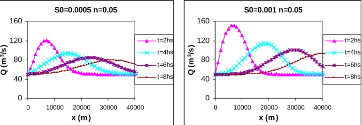
S0=0.0005 n=0.05
0 40 80 120 160
0 10000 20000 30000 40000
x (m )
Q (
m
3/s
) t=2hs
t=4hs
t=6hs
t=8hs
S0=0.001 n=0.05
0 40 80 120 160
0 10000 20000 30000 40000
x (m )
Q (
m
3/s
) t=2hs
t=4hs
t=6hs
t=8hs
Figure 2. Propagation of the dynamic wave, for different bed slopes.
values equal to 0.0005 and 0.001. It is observed that as larger the bed slope is, the large will be the pick flow and the fast will be the wave propagation.
These results show that the hydraulic parameters related with the roughness and with the bed slope of the channel play an important control on the process of the dynamic wave propagation.
n=0.01 S0=0.001
0 2 4 6 8 10 12
0 10000 20000 30000 40000
x (m )
C (
m
g
/l
)
t=1h
t=2hs t=4hs t=6hs
t=8hs
n=0.1 S0=0.001
0 2 4 6 8 10 12
0 10000 20000 30000 40000
x (m )
C (
m
g
/l
) t=2hs
t=4hs
t=6hs
t=8hs
Figure 3. Behavior of concentration field for different roughness.
The figure 3 shows the effect of a dynamic wave on the process of transport of a pollutant substance, in a natural channel. Simulations were accomplished with different roughness n=0.01 and n=0.1, considering a same
bed slope S0=0.01. It is noticed that as larger the roughness is, the smaller will
be the celerity of the dilution wave.
Through the figure it can be noticed that with the propagation of the flood wave, a dilution wave propagates with the same frequency and with, approximately, the same velocity.
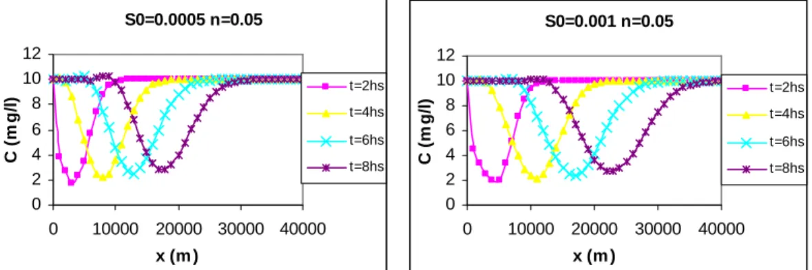
S0=0.0005 n=0.05
0 2 4 6 8 10 12
0 10000 20000 30000 40000
x (m )
C (
m
g
/l
) t=2hs
t=4hs
t=6hs
t=8hs
S0=0.001 n=0.05
0 2 4 6 8 10 12
0 10000 20000 30000 40000
x (m )
C (
m
g
/l
) t=2hs
t=4hs
t=6hs
t=8hs
Figure 4. Behavior of the concentration field for different bed slope.
In the simulations of the figure 4 it was considered just one value for n and
different S0. It is verified that the behavior of the dilution wave also
corresponds the propagation of the dynamic wave. The graph shows that the behavior of this dilution wave is, directly, related with the hydraulic characteristics of the natural river.
previously and they show that as bigger n the bigger will be the dilution pick. Thus, it is ended that the dilution capacity, in the point of view of intensity, is proportional to the resistance caused by the friction in the wall of the channel.
t = 2 hs
0 2 4 6 8 10 12
0 10000 20000 30000 40000
x (m )
C (
m
g
/l
)
n=0.01
n=0.05
n=0.1
t = 4 hs
0 2 4 6 8 10 12
0 10000 20000 30000 40000
x (m )
C (
m
g
/l
) n=0.01
n=0.05
n=0.1
Figure 5. Behavior of the concentration field for different roughness.
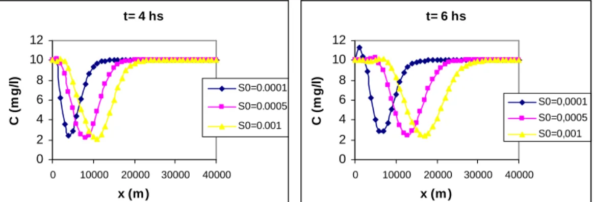
t= 4 hs
0 2 4 6 8 10 12
0 10000 20000 30000 40000
x (m )
C (
m
g
/l
)
S0=0.0001
S0=0.0005
S0=0.001
t= 6 hs
0 2 4 6 8 10 12
0 10000 20000 30000 40000
x (m )
C (
m
g
/l
)
S0=0,0001 S0=0,0005
S0=0,001
Figure 6. Behavior of concentration field for different bed slope and time.
The figure 6 shows the results obtained through the simulations for different values of the bed slope in the times of four six hours. The results show that this parameter plays an opposite way that carried out by the roughness coefficient. In this case, as bigger the bed slope is, the larger will be the celerity of the dilution wave.
Another aspect that should be observed in the figure 6 is that as bigger the bed slope is, the larger will be the dilution pick. However, comparing the graphs of those figures, it is noticed that there is no dissipation of energy and the dilution capacity stays along the time. In other words, for 4 hours and 6 hours of propagation, the dilution picks continue very close.
4. Conclusions
capacity to present results, as well as in the capacity to answer, efficiently, to different sceneries of studies.
The presented results allow concluding that the bed slope and the roughness coefficient play important game in the dispersion process of pollutant in rivers. Through the graphs it is noticed that the effect of the roughness is more intense than the effect of the bed slope.
In the case of the roughness as bigger are their values, the larger will be the dilution pick. Therefore, it is ended that the dilution capacity, in the point view of intensity, is proportional to the resistance to the flow in the channel. On the other hand, for the bed slope, as larger is its value, the bigger will be the capacity of dilution of the rivers, in spite of this variation not be so significant.
References
Bajracharya, K. Barry, D.A. (1999). Accuracy Criteria for Linearised Diffusion Wave Flood Routing, Journal of Hydrology, 195, p. 200-217, Elsevier.
Barry, D.A., Bajracharya, K. (1995). On the Muskingum-Cunge Flood Routing Method. Environmental International, vol. 21, n. 5, p. 485-490, Elsevier.
Branco, S. M. (1991). Hidrologia Ambiental, vol. 3, Edusp, ABRH.
CHAPRA, S. C.; RECKHOW, K. H., (1983). Engineering Approaches for Lake Management, Vol. 2: Mechanistic Modeling, Butterworth Publishers.
Chapra, S. C. (1997). Surface Water-quality Modeling, McGraw-Hill. Chow, V. T. (1988).Applied Hydrology, New York: McGraw-Hill, 572p.
Fischer, H. B. (1979). Mixing in Inland and Coastal Water, Academic Press, Inc.. JAMES, A. (1978). Mathematical Model in Water Pollution Control, John Wiley &
Sons.
Keskin, M. E. And Agiralioglu, N. (1997). A Simplified Dynamic Model for Flood Routing in Rectangular Channels, Journal of Hydrology, 202, p. 302-314, Elsevier.