A numerical model to investigate the polarisation azimuth of ULF waves through an ionosphere with oblique magnetic fields

SRef-ID: 1432-0576/ag/2005-23-3457 © European Geosciences Union 2005

Annales

Geophysicae

A numerical model to investigate the polarisation azimuth of ULF

waves through an ionosphere with oblique magnetic fields

M. D. Sciffer, C. L. Waters, and F. W. Menk

School of Mathematical and Physical Sciences and CRC for Satellite Systems, The University of Newcastle, New South Wales, Australia

Received: 27 May 2005 – Revised: 12 October 2005 – Accepted: 17 October 2005 – Published: 21 December 2005

Abstract. A one dimensional, computational model for the propagation of ultra low frequency (ULF; 1–100 mHz) wave fields from the Earth’s magnetosphere through the iono-sphere, atmosphere and into the ground is presented. The model is formulated to include solutions for high latitudes where the Earth’s magnetic field, (B0), is near vertical and

for oblique magnetic fields applicable at lower latitudes. The model is used to investigate the wave polarisation azimuth in the magnetosphere compared with the ground wave fields, as a function of the dip angle ofB0. We find that for typical

ULF wave scale sizes, a 90◦rotation of the wave polarisa-tion azimuth from the magnetosphere to the ground occurs at high latitudes. However, this effect does not necessarily occur at lower latitudes in all cases. We show that the de-gree to which the wave polarisation azimuth rotates critically depends on the properties of the compressional ULF wave mode.

Keywords. Ionosphere (Ionosphere-atmosphere inter-actions; Wave propagation) – Magnetospheric physics (Magnetosphere-ionosphere interactions)

1 Introduction

Ultra-low frequency (ULF) plasma waves in the 1–100 mHz range are ubiquitous in the Earth’s magnetosphere. Ground based sensors, such as sensitive magnetometers, detect these waves and the observations are used to deduce ULF wave generation and propagation mechanisms which in turn re-veal the dynamics of the magnetosphere. For detection at the ground, ULF wave energy must pass through the iono-sphere and atmoiono-sphere. A thorough understanding of ULF wave propagation through the ionosphere/atmosphere sys-tem is important for using ULF wave properties to remote sense the magnetosphere. Even though the wavelengths are much larger than the height of the ionosphere, there are Correspondence to:C. L. Waters

(colin.waters@newcastle.edu.au)

major alterations to the wave characteristics as they leave the highly ionoised medium in the magnetosphere and propagate through the neutral atmosphere to the ground.

The properties of ULF waves in the ionosphere and at-mosphere have been examined for both vertical (or near-vertical) and horizontal orientations of B0 (Hughes, 1974;

Hughes and Southwood, 1976; Zhang and Cole, 1994). A combined analytic and numerical study of ULF wave prop-agation from the magnetosphere through the ionosphere to the ground was given by Hughes (1974) who examined the problem using the Maxwell equations. The analytic solu-tions used height integrated conductivities and approximated the ionosphere as a thin current sheet. Ideal MHD conditions were used to describe the behaviour of the waves above the ionosphere current sheet. Hughes (1974) examined the ULF wave fields for vertical and oblique geomagnetic fields ap-propriate to high latitude regions, and showed how the wave fields may be “screened” by the ionosphere. In particular, for an incident shear Alfv´en mode ULF wave with the perturba-tion magnetic field in the east-west (y) direcperturba-tion in the mag-netosphere, (i.e.kx=0), the wave magnetic field at the ground was shown to be in the north–south (x) direction. One con-clusion of Hughes (1974) was that wave reflection at the top of the ionosphere was very efficient with a reflection coeffi-cient≈1. More recently, the ionosphere has been shown to behave more inductively for various frequencies, conductiv-ity profiles and wavenumbers (Yoshikawa et al., 2002; Sciffer et al., 2004) which lead to smaller reflection coefficients.

Hughes (1974) also developed a numerical model which examined the case where the geomagnetic field was oblique andkx6=0. However, the condition, _Vaω≪k⊥ was imposed and the polarisation of the shear Alfv´en wave had no de-pendence on the vertical wave number, kz, in the magne-tosphere/ionosphere boundary condition. This makes the solutions valid only for near vertical B0. For dip angles

of the geomagnetic field corresponding to lower latitudes, there is a contribution ofkxalong the direction ofB0which

may be greater than _Vω

wavenumber,k, was assumed to be<₁₀₀1 km−1and the inci-dent wave from the magnetosphere was limited to the shear Alfv´en mode. In the present paper we investigate the ULF wave solutions with detailed altitude information for mid to low latitude geomagnetic field dip angles and allow for an in-ductive ionosphere, small wave numbers and incident com-pressional mode energy.

Zhang and Cole (1994, 1995) presented a numerical model of ULF wave propagation through the ionosphere for verti-cal and horizontalB0 cases. They formulated the solution

as a one dimensional (1-D), electromagnetic wave propaga-tion model which was solved as a boundary value problem. Rather than impose ideal MHD conditions, the top boundary was assumed to be a uniform cold plasma with finite con-ductivity. This formulation allowed the incident wave mode mix to be specified in terms of the wave polarisation at the top boundary, with separation into upward and downward wave solutions calculated from constraints at the top bound-ary. Zhang and Cole (1995) examined the case whereB0was

horizontal, relating to equatorial regions where the formula-tion considered only the incident compressional mode wave. Zhang and Cole (1994) examined the case for a vertical geo-magnetic field while allowing for a mixture of incident ULF wave modes. The magnetosphere medium was described by resistive plasma equations with finite conductivity in the top-side region giving complex wave numbers and elliptically polarised waves. The effect of numerical swamping (e.g. Pit-teway, 1965) due to the compressional mode was avoided by Hughes (1974) by limitingk⊥≤₁₀₀1 km−1. This ensured the evancesent decay length was large so that the growing compressional mode solution (which is unphysical) did not dominate the numerical solution. This condition was sub-sequently removed in Hughes and Southwood (1976) where the two wave modes were kept orthogonal.

The extension of modeling ULF wave propagation through the ionosphere for any dip angle ofB0was presented as an

analytic formulation by Sciffer and Waters (2002). The aim of the present paper is to extended that work for obliqueB0to

include a realistic height dependent conductivity tensor. We keep the finite conductivity plasma condition in the magneto-sphere top boundary as described by Zhang and Cole (1994) and include non verticalB0. The effect of obliqueB0on the

well known 90◦rotation in polarisation azimuth of the ULF wave field between the magnetosphere and ground is exam-ined to determine if these effects remain valid for an oblique geomagnetic field geometry.

2 Mathematical formulation

A ULF wave incident from the magnetosphere may be de-scribed as an electromagnetic disturbance. We assume that the magnetosphere and ionosphere plasma is overall electri-cally neutral and that the zero order electric field,E0, is zero.

The relevant Maxwell equations are,

∇×E = −∂B

∂t (1)

∇×H =J+∂D

∂t (2)

where the current density,Jand magnetic flux density,Bare given by

J = ¯σE (3)

B=µH (4)

whereσ¯ is the conductivity tensor.

A Cartesian coordinate system is used whereXis north-ward,Y is westward andZis radially outward from the sur-face of the Earth. The geomagnetic field,B0, lies in theXZ

plane at an angle,I to the horizontal. The ULF wave electric and magnetic perturbation fields areeandbrespectively so that

B=B0+b=(B0cos(I ),0, B0sin(I ))+(bx, by, bz) (5) E=E0+e=(ex, ey, ez) (6) Fourier analysing in time and space with an ei(kxx+kyy−ωt )

dependence, the governing equations in component form be-come

0=ikyǫ13

ǫ33

bx−

_∂

∂z+ ikxǫ13

ǫ33

by−i

" k2_y

ω− ω c2

ǫ11−

ǫ31ǫ13

ǫ33

# ex

+i _k

xky

ω + ω c2

ǫ12−

ǫ32ǫ13

ǫ33

ey (7)

0=

_∂

∂z+ ikyǫ23

ǫ33

bx−

ikxǫ23

ǫ33

by+i

_k

xky

ω + ω

c2

ǫ21−

ǫ31ǫ23

ǫ33

ex

−i "

k_y2 ω−

ω c2

ǫ22−

ǫ32ǫ23

ǫ33

#

ey (8)

0= iω−c

2_k2 y

ωǫ33

!

bx+

ic2kxky

ωǫ33

!

by+

ikyǫ31

ǫ33

ex

−

_∂

∂z+ ikyǫ32

ǫ33

ey (9)

0=ic

2_k xky

ωǫ33

bx+ iω−

c2k_x2 ωǫ33

!

by−

_∂

∂z+ ikxǫ31

ǫ33

ex

+

_ik

xǫ32

ǫ33

ey. (10)

This is a system of four, first order differential equations in-volving the spatial derivatives in altitude,z. Theezandbz wave components are given by

ez =

−kyc2

ωǫ33

bx+

kxc2

ωǫ33

by−

ǫ31

ǫ33

ex−

ǫ32

ǫ33

ey (11)

bz =

ky

ωex− kx

Theǫij are theith row andjth column of the dielectric tensor,ǫ¯, which is related to the conductivity tensor by

¯

ǫ= ¯I− i

ǫ0ω

¯

σ (13)

whereI¯is the identity tensor.

In specifying the boundary conditions we assume that the plasma above the region where the equations are solved is cold and uniform but has finite conductivity. An examination of the wave modes which can propagate above the ionosphere and traverse the upper boundary is in order. The nature of the wave modes which can exist in a magnetised cold plasma has been examined by a number of authors (e.g. Stix, 1962; Pitteway, 1965; Zhang and Cole, 1994). Since our model assumes a resistive plasma, there are no pure shear Alfv´en (transverse) or pure fast (compressional) wave modes in the MHD sense. However, we will identify the wave mode that has the majority of its Poynting flux in the direction ofB0

as the “shear Alfv´en” mode and the wave with the majority of its Poynting flux in the direction ofkf as the “compres-sional” or fast mode.

Taking the curl of (1) and using (2), the matrix which de-fines the dispersion relation for the resistive plasma is

k·k−k2I¯+k₀2ǫ¯·E=0 (14) Alternatively, Eq. (14) may be written in terms of a matrix,

9(kz)as

9(kz)·E=0 (15)

where k=i(kx, ky, kz) and k0=ω(µ0ǫ0) 1

2_{, the free space} wavenumber.

Whenkxandkyare specified, the determinant of9may be written as a quartic inkz. For non-trivial solutions the deter-minant of9must be zero. The four roots of det(9)=0 rep-resent the vertical wavenumbers for each wave mode which may exist in the region above the computational domain. De-noting the direction set (incident or reflected) byd and the wave mode set (Alfve’n or fast) bym then for each root,

kd_z,m, we may solve for the electric field, expressed in unit vector form as described in the next section. The character-istic equation is

9(kd_z,m)·P =λP =0 (16) whereλis the eigenvalue of the matrix9 evaluated at each of the roots,kd_z,m. The unit magnitude eigenvector

∧ Pd_m as-sociated withλ=0 represents the polarisation of the electric field of the corresponding wave mode,m. We shall denote shear Alf´ven wave modes as

∧ Pra and

∧

Pia, where the i and

r indicate whether the vertical Poynting flux is towards or away from the surface of the earth. Similarly, an incident and reflected compressional wave mode are identified as

∧ Pi_f

and ∧ Pr

f, respectively.

The compressional wave mode solutions for det(9)=0 for a givenkx,ky and conductivity profile, are denoted askr_z,f and k_z,fi and are generally complex. The real part indi-cates the propagating nature of the mode while the imag-inary part indicates the spatial scale of the wave mode. For ideal MHD conditions, the compressional mode disper-sion relation gives vertical wavenumbers which are purely imaginary, an “evanescent” mode or purely real, a “prop-agating” mode. For complex kz, the waveform oscillates while diminishing with distance. In the following sections the wave frequencies are <100 mHz and we find that the solution of det(9)=0 for the compressional mode vertical wavenumber is similar to the ideal MHD case. Therefore, we use the ideal MHD terminology where the fast mode is ’propagating’ if|Re(kz,f)|≫|Im(kz,f)|and “evanescent” if

|Re(kz,f)|≪|Im(kz,f)|. Also, similiar to ideal MHD, for a fixedkx,ky and conductivity there is a “critical frequency” at which the vertical wavenumber of the fast mode transitions between “propagating” and “evanescent”.

The top boundary includes any mixture of shear Alfv´en and compressional mode disturbances. The total electric field Et, is comprised of both downward (incident) and upward (reflected) components of both wave modes so that the total electric field at the top of the computational domain is given by   ex ey ez 

=αr

∧ Pr_a+αi

∧ Pi_a+βr

∧ Pr_f +βi

∧

Pi_f (17)

Theαandβare amplitude factors for each of the wave modes entering or leaving the solution region. This superposition of the magnetosphere electric fields allows the wave fields and their derivatives to be expressed in terms of the composition of MHD wave modes present above the top boundary. The polarization of each wave mode is contained in theP∧.

Given that we have linearized the problem in the form

ei(kxx+kyy)_{, we may write the x and y components of the total} electric field and the derivatives as

Ex=αi ∧

P_x,ai +βi

∧

P_x,fi +αr

∧

P_x,ar +βr

∧

P_x,fr (18)

Ey=αi ∧

P_y,ai +βi

∧

P_y,fi +αr

∧

P_y,ar +βr

∧

P_y,fr (19)

∂Ex

∂z =ik

i z,aα

i _P∧i x,a +ik

i z,fβ

i _P∧i x,f

+ikr_z,aαr

∧

P_x,ar +ik_z,fr βr

∧

P_x,fr (20)

∂Ey

∂z =ik

i z,aαi

∧

P_y,ai +iki_z,fβi

∧

P_y,fi

+ikr_z,aαr

∧

P_y,ar +ik_z,fr βr

∧

The total electric field and its derivatives can now be written in terms of the matrix, where

    Ex Ey ∂Ex ∂z ∂Ey ∂z     =[]·     αi βi αr βr     =           ∧

P_x,ai

∧

P_x,fi

∧

P_x,ar

∧

P_x,fr

∧

P_y,ai

∧

P_y,fi

∧

P_y,ar

∧

P_y,fr

ik_z,ai

∧

P_x,ai ik_z,fi

∧

P_y,fi ik_z,ar

∧

P_x,ar ik_z,fr

∧

P_x,fr

ik_z,ai

∧

P_y,ai ik_z,fi

∧

P_y,fi ik_z,ar

∧

P_y,ar ik_z,fr

∧

P_y,fr               αi βi αr βr     (22)

To obtain the upward and downward components of the total wave electric field we need to invert the matrixso that

    αi βi αr βr    

=[]−1·

    Ex Ey ∂Ex ∂z ∂Ey ∂z     (23)

The incident wave amplitude (αi and βi) can now be ex-pressed in terms of the total electric field and used to specify the upper boundary conditions:

αi =da

Ex, Ey,

∂Ex ∂z , ∂Ey ∂z (24)

βi =df

Ex, Ey,

∂Ex ∂z , ∂Ey ∂z (25) whereda anddf are the corresponding rows of the ma-trix−1. This requires values for the incident amplitudes of both wave modes. In specifyingαi andβi we also spec-ify the mode mix of the incident disturbance. An advantage of this procedure is that the expression for the amplitude of the reflected modes at the top boundary,αr _andβr _{may be} calculated from Eq. (23) after the solution forEt has been obtained.

Since (7) to (10) describe a system of four equations, a further two boundary conditions are required. For these we assume the Earth is a uniform, homogeneous conductor with finite conductivity which implies

∂ex

∂z −γ σg, kx, ky, ω

ex=0 (26)

∂ey

∂z −γ σg, kx, ky, ω

ey=0 (27)

whereγ sets the ground to be a uniform, homogeneous con-ductor with conductivityσg. The solutions which satisfy this condition are imposed so that the ULF wave is attenuated beneath the surface of the Earth. For the results presented in this paper we have setσg=10−2Mho/m.

With these boundary conditions, and a second order fi-nite differencing scheme we solved the boundary value prob-lem using the Numerical Algorithms Group (NAG) package number FO4ADF. The computational domain was chosen

Fig. 1. The direct (solid), Pedersen (dotted)) and Hall (dashed) conductivities for solar minimum and maximum following Hughes (1974). An incident 16 mHz (ω=0.1) ULF wave was used.

to be 1000 km in altitude with a uniform grid spacing of 2 km. The composition of the atmosphere and ionosphere were calculated from the thermosphere model based on satel-lite mass spectrometer and ground-based incoherent scatter data (MSISE90), (Hedin, 1991) and the International Ref-erence Ionosphere (IRI-95) models. The International Ge-omagnetic Reference Field (IGRF-95) was used to provide values forB0. Data for the collision frequencies below 80 km

were extrapolated to the ground using the expressions in Ap-pendix A. The eigenvectors,P, in Eq. (16) were found using the NAG routine F02GBF, while the roots of Eq. (14) were computed using the NAG routine C02AFF.

3 ULF wave polarisation azimuth in the horizontal plane

Validation of the computations was achieved by compar-ing with published results and with the analytic solutions developed by Sciffer and Waters (2002) and Sciffer et al. (2004). In this section, results from a comparison with those of Hughes (1974) are presented, followed by a study of the horizontal polarisation of the magnetic perturbations of ULF waves through the ionosphere as a function of latitude.

maximum conditions, ULF wave frequency ofω=0.1 and a B0dip angle, I=70◦. For these conditions, the direct,

Peder-sen and Hall conductivities, including the kinetic terms are shown in Fig. 1. Above 200 km, the conductivity alongB0 (direct conductivity) is of order 1×107times larger than the Pedersen and Hall conductivities. However, the Pedersen and Hall terms give rise to the anisotropic ionosphere conductiv-ity, allowing conversion of the ULF modes. The conductivity has been “ramped” down so that it decreases with decreasing altitude in the atmosphere as described by Hughes (1974). The small but finite conductivity in the atmosphere is dis-cussed further in Sect. 4.

Figure 2 shows the electric and magnetic ULF wave fields for an incident shear Alfv´en-like wave mode. While the de-tails of the ionosphere used in Hughes (1974) are not pro-vided, the wave fields are very similar to his Fig. 4. Com-putation of our model using the same parameters as other examples presented in Hughes (1974) also agreed with their results. Results from our model were also compared with those in Zhang and Cole (1994), Hughes and Southwood (1976) and Poole et al. (1988) and found to reproduce the respective published plots. This shows that for the condition that specifies an incident shear Alfv´en mode only, there is lit-tle difference between assuming that the medium at the top boundary consists of a resistive plasma compared with ideal MHD conditions. This also implies that at these frequencies, the ideal MHD formulation in the analytic model of Sciffer and Waters (2002) is a reasonable approximation. For refer-ence, the electric fields of the ULF waves from Sciffer and Waters (2002) are

ef =β

−kysin(I ), kxsin(I )−kz,fcos(I ), kycos(I )(28) for the compressional mode and

ea=α(kxsin(I )−kz,acos(I ))sin(I ),

ky,−(kxsin(I )−kz,acos(I ))cos(I ) (29) for the shear Alfv´en mode. The 90-deg rotation (NDR) effect of wave polarisation azimuth described by Hughes (1974) can be seen in the azimuth angle shown in Fig. 2. Polarisation azimuth for a verticalB0

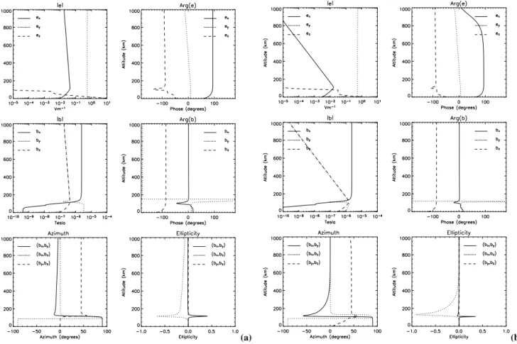
Figure 2 shows that the ULF magnetic wave fields change in amplitude and phase as a function of altitude. A well known property of ULF wave fields is the polarisa-tion azimuth in the horizontal plane, calculated using the wave polarisation parameters from bx and by. The sim-plest case is for vertical B0 and small kx. Figure 3a shows the classic case where an incident shear Alfv´en wave with kx=1×10−10m−1 and ky=1×10−6m−1 is modeled. The Alfv´en speed at 1000 km altitude is 2.8×106ms−1. This gives kz,a=ω/Va=3.6×10−8m−1 for the incident shear Alfv´en mode. From Eqn. (29), the incident shear Alfv´en mode has an electric field vector proportional to

ea=(kx, ky,0) with the larger ey clearly seen in Fig. 3a. Therefore, the magnetic perturbation associated with the shear Alfv´en mode is largely in thebx component and the compressional mode hasbyandbzcomponents.

Fig. 2. ULF wave fields and polarisation azimuth for

kx=10−10m−1,ky=10−6m−1andω=0.1 (f≈16 mHz). The dip angle is 70◦. Compare with Fig. 4. in Hughes (1974).

Comparing with Fig. 2, theex andey components of the electric field in Fig. 3a are similiar, while the vertical electric field differs due to the inclination of the background mag-netic field in Fig. 2. For verticalB0, ez≈0 since the field aligned component of the electric field is small where the direct conductivity is large. The ULF wave magnetic fields vary in a similar fashion compared with those in the oblique field in Fig. 2. This is due toez≈0 for the vertical field and some small differences in the phasing of the fields. The po-larisation azimuth rotation in thebx andby components in both Figs. 2 and 3a are very similiar. The explanation for this effect in terms of∇×bhas been given by Southwood and Hughes (1983). This polarisation rotation of the wave fields occurs over a narrow range in altitude near 120 km. The wave goes from linearly polarized to elliptically polarised in a right handed (clockwise) sense near 120 km altitude returning to linear polarisation in the atmosphere.

Figure 3b has an incident shear Alfven wave where

(a) (b)

Fig. 3. Polarisation azimuth computed frombxandbyfor a verticalB0. In(a)kx=10−10m−1andky=10−6m−1, similar to Fig. 2 while in(b)kx=10−10m−1andky =10−5m−1for frequency off =16 mHz at solar minimum withVa=2.8×106ms−1at 1000 km altitude. The wave fields are X (solid), Y (dotted) and Z (dashed).

ionosphere/atmosphere results in wave reflection and the re-sulting ionosphere current system gives rise to a compres-sional mode which forms a surface wave in this region (Yoshikawa and Itonaga, 2000; Sciffer and Waters, 2002). The evanescent nature of the compressional mode for the specified scale size is shown in the decay in amplitude with altitude. The wave field components of the shear Alfv´en mode and the phasing of the fields are not significantly al-tered. The polarisation azimuth rotation in the horizontal magnetic field components also shows a NDR. However, in this case the NDR develops over an altitude range starting at 500 km and reaching 90◦_{near 120 km, the ionospheric} E-region. Therefore, a straightforward rotation of ULF netic fields projected onto the ground, by rotating the mag-netic field through 90◦ may not be appropriate. This effect is particularly pertinent when using radar or low Earth or-bit satellite data where measurements in space may be lo-cated within the region where the NDR has partially begun. The ellipticity is not significantly altered by the more gradual change in polarisation azimuth with altitude in Fig. 3b.

Figure 3 has shown that the ULF wavenumber affects the altitude range over which the NDR occurs. The polarisa-tion azimuth computed from thebxandbyULF wave fields

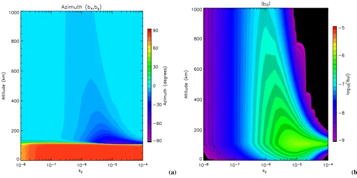
as a function of both altitude and wavenumber in a vertical B0is shown in Fig. 4a for solar maximum conditions where Va=6.5×105ms−1at 1000 km altitude. The incident shear Alfv´en like wave has a dominantbx component. The ma-jor axis of the horizontal polarisation ellipse changes as a function of altitude and wavenumber above the ionosphere E-region. Below this, the orientation of the major axis is rotated into the positiveydirection (west). Askyincreases the ver-tical nature of the compressional mode changes from propa-gating to evanescent. From Eq. (14) the vertical wavenumber of the compressional mode at 1000 km, in this case, is pre-dominately propagating forky≤1.5×10−7m−1.

(a) (b)

Fig. 4. (a)The polarisation azimuth computed frombx andby, for a frequency of 16 mHz and dip angle ofI=90◦at solar maximum. The wavenumbers arekx=10−10m−1andkyvarying between 10−8and 10−4m−1.(b)The amplitude of the field aligned (compressional) component of the ULF wave magnetic field (bzin the case of a vertical field) for the parameters used in (a).

In order to see this effect, Fig. 4b shows the field aligned component of the ULF wave magnetic field, which isbzfor a verticalB0. Thebzcomponent is a good indicator of how much compressional mode is present at a given altitude. The region where the compressional mode is generated can be seen to be near the ionosphere E-region where the Pedersen and Hall conductivities are large. As the wave number in-creases, the amplitude of the compressional magnetic field at 120 km altitude increases until it achieves a maximum value atky≈1×10−5m−1. The amount of compressional mode as a function of altitude depends on the conversion coefficient,

|AF|(Sciffer and Waters, 2002) of the wave modes and the efolding distance of the vertically evanescant compressional mode. Figure 4b shows this behavior as a reduction in am-plitude ofbzabove (and below) the ionosphere E-region for the larger values of the horizontal wavenumber. The impor-tant factors are the amount of converted compressional mode and thee folding distance of the mode that determine the height at which the NDR will start, as well as the altitude dependence of the polarisation ellipse major axis rotation for the ULF wave. Since the rotation depends on the conversion between the ULF wave modes, parameters such as the iono-sphere conductivities, wave frequencies and dip angle play an important part in determining these factors, as discussed in Sciffer et al. (2004).

4 Polarisation azimuth for ObliqueB0

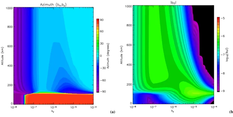
The effect of a non verticalB0on the ULF wave polarisation

azimuth for solar maximum ionosphere conditions is shown

in Fig. 5a. The parameters are the same as those for Fig. 4a except that the inclination ofB0is now 70◦. The change in

azimuth with altitude and wavenumber has features in com-mon with Fig. 4a, particularly for wavenumbers greater than

ky≈2×10−7m−1. The slight differences are due to the de-pendence of the wave mode conversion coefficients on theB0

dip angle as explained by Sciffer and Waters (2002). How-ever, for small wavenumbers, we have the possibility that the NDR does not occur. For the parameters chosen, this is for horizontal wavenumbers,ky<2×10−7m−1, where the com-pressional mode is propagating. The polarisation azimuth does not change with altitude above the ionosphere E-region, as the by wave component does not decrease in amplitude with height.

Below 120 km, we need to address the NDR effect as ex-plained in Southwood and Hughes (1983). Basically, the rea-soning considered ∇×b=0 in the neutral atmosphere com-pared with ∇×b6=0 in the magnetosphere. The change in

∇×bfrom the magnetosphere through to the atmosphere is manifested by a rotation of the wave fields by 90◦_{. The curl} of the horizontal magnetic wave fields is

(∇ ×b)_z=µ0jz−i

ω

c2ez (30)

(a) (b)

Fig. 5. Polarisation azimuth between the ULF wavebxandbycomponents for a frequency of 16 mHz, dip angle ofI=70◦and solar max-imum ionosphere conditions.(a)Wavenumbers arekx=10−10m−1andkyvarying between 10−8m−1and 10−4m−1. (b)The amplitude of the field aligned (compressional) component of the ULF wave magnetic field for the parameters in (a).

shown in Fig. 1. To remedy this situation, the conductivities were ramped down more steeply than those in Hughes (1974) in the lower regions (≤60 km) of the atmosphere. This re-duced the conduction current prore-duced by the ULF wave in the atmosphere and the NDR was restored for the small wavenumbers in Fig. 5.

Figure 5b shows the amplitude of the ULF wave magnetic field component that is aligned alongB0. Compared to the

vertical case shown in Fig. 4b, more compressional mode appears for the smaller wavenumbers. Since the compres-sional mode at these wavenumbers is propagating, or has a large efolding distance, there is a greater proportion of compressional mode energy from 120 km altitude and higher for non vertical dip angles. As the wavenumber increases the evanescent nature of the mode becomes important and the amplitude of the field aligned ULF wave magnetic field decreases exponentially, similar to the verticalB0case. Polarisation azimuth rotation for constant azimuthal wavenumber

A common parameter used to describe the propagation prop-erties of ULF waves is the azimuthal wavenumber, also known as themnumber. From Olson and Rostoker (1978),

ky=

m

2π REcos(θg)

(31) where Re is the Earth radius and θg is the geographic lat-itude. For example, for m=3 at mid latitudes (θg≈50◦),

ky≈1×10−7m−1while theB0dip angle, I≈80◦. In order

to gain some insight into the latitudinal dependence of the

ULF wave polarisation azimuth, the polarisation azimuth ro-tation was calculated as a function of altitude and geographic latitude for a constant wave frequency and constantm. The ionosphere conductivities were calculated at each latitude us-ing the IRI-95 model for 10:00 LT on 28 September 2000 along the 150◦geographic longitude.

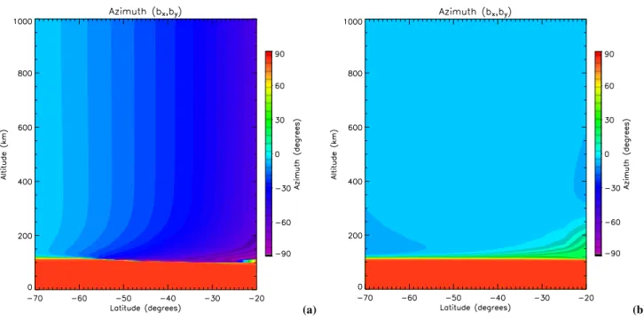
Figure 6a shows the results forf=25 mHz and m=3. The ULF wave polarisation azimuth rotation depends on geo-graphic latitude, over the –70◦ _{to –20}◦ _{latitude range, k}

y varies from 2×10−7to 8×10−8m−1 at the lowest latitude. The conductivities were similar across all latitudes. The crit-ical frequency at which the compressional mode starts to propagate for these latitudes is≈20 mHz. The non-NDR ef-fect at low latitudes depends on the conversion coefficients of the wave modes, a feature that is discussed later. If the ULF wave frequency is below the critical frequency, the ULF wave undergoes a NDR at all latitudes. Figure 6b shows the results form=12. The critical frequency is now shifted up to

≈80 mHz. This gives the usual NDR effect at all latitudes with a sharp change near the ionosphere E-region since the compressional wave mode is highly evanescent for these pa-rameters.

(a) (b)

Fig. 6. ULF wave polarisation azimuth computed from thebxandbycomponents for a frequency of 25 mHz. The IRI-95 model parameters were chosen for conditions on 28 September 2000 for the 160◦geographic longitude at 10:00 LT. The geographic latitudes vary between 70◦ and 20◦south. The north-south wavenumber iskx=10−10m−1. The azimuthal wavenumber,(a)m=3,(b)m=12.

maximum conditions, the results for solar minimum condi-tions were also computed and show similar features. Es-sentially, the reduced conductivities for solar minumum and the larger Alfven speeds shift the features described above to smaller values of k⊥. For example, the most gradual change in the polarisation azimuth with altitude in Fig. 4a is for ky≈1×10−6m−1. For solar minimum, the figure appears essentially the same except that the correspond-ing change in the polarisation azimuth with altitude occurs aroundky≈1×10−7.

5 Discussion

In order to further explore wave polaristaion azimuth rota-tion for obliqueB0, we can compare the results with the

an-alytic model described in Sciffer et al. (2004). The numer-ical model described in the present paper derives the ULF wave fields in a different and therefore independent manner to the analytic formulation presented by Sciffer et al. (2004). The analytic model may be used to verify the results of the numerical model, provide insights into the reflection prop-erties of the ionosphere and examine the ULF wave fields in more detail. The analytic model was formulated to allow the separation of incident and reflected components of the shear Alfv´en and compressional mode waves. It uses height integrated conductivities, replacing the ionosphere by a cur-rent sheet, so we expect the details around the ionosphere E-region to be different compared with the numerical calcula-tions. However, due to the wavelengths involved the analytic and numerical model results should be similar away from the

ionosphere E-region. One further difference between the an-alytic compared with the numerical formulation concerns the frequency. For Pc1 studies (>0.2 Hz), the slab construction of the analytic model does not describe features that occur due to the variation of the topside ionosphere with altitude. However, such details can be described using the numerical model presented in this paper.

Taking the obliqueB0case presented in Fig. 5, the

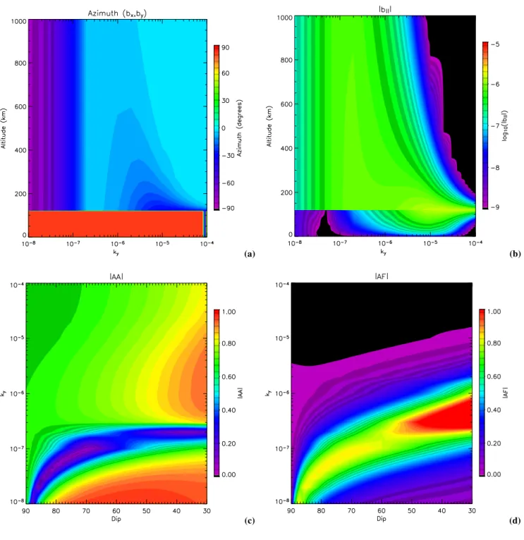
corre-sponding results from the analytic model are shown in Fig. 7. The parameters were chosen to closely represent those used in Fig. 5. The current sheet was placed at d=120 km, a height corresponding to the ionosphere E-region and the ULF wave frequency is 16 mHz. The height integrated conductivities are6d=106S,6P=6.2 S and6H=7.6 S, which correspond with solar maximum conditions for the data in Fig. 5. A change in polarisation azimuth from the magnetosphere to the atmosphere is seen for all wavenumbers in Fig. 7 as the analytic model specifies an atmosphere with zero conduction current. The variation of polarisation azimuth and the field aligned component of the ULF wave with wavenumber and altitude for the numerical model (Fig. 5a) and the analytic model (Fig. 7) are similar. This confirms that the analytic model is a good approximation to the numerical model for these frequencies.

(a) (b)

(c) (d)

Fig. 7. Results from the analytical model of Sciffer et al. (2004). The parameters used were:Va= 6.4×105ms−1,kx=1×10−10m−1and

kyvarying between 10−8m−1and 10−4m−1. The current sheet altitude was d=120 km and the frequency, 16 mHz. The height integrated conductivities were60=106S,6p=6.2 S and6h=7.6 S.(a)Polarisation azimuth rotation (bx,by) for dip,I=70◦. (b)Amplitude of the field aligned (compressional) component of the ULF wave for dip,I=70◦.(c)Absolute value of the reflection ratio,AAversuskyand dip angle.(d)Same as (c) but for the conversion coefficient,AF (shear Alfv´en to compressional wave mode).

Fig. 7b. Therefore, there will be little change in azimuth with altitude as seen in Fig. 6a. Figures 7c and 7d show the shear Alfv´en wave reflection coefficient, |AA| and the shear Alfv´en to compressional mode conversion coefficient,

|AF|coefficients from Sciffer and Waters (2002) as a func-tion ofkyand dip angle. At –20◦latitude, the dip is≈45◦. For 1×10−8≤ky≤2×10−7m−1, the conversion from shear

magnetosphere compared with the ground. In the case of a verticalB0 the conversion coeffecient, |AF| is very small

and hence there is very little compressional component for smallkyin Fig. 4b.

The second region in Fig. 7 is for

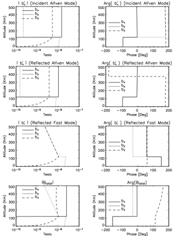
2×10−7≤ky≤2×10−5m−1. The effect on the ULF wave polarisation azimuth depends on the relative magni-tudes of each ULF wave mode. Forkx≈0 the shear Alfv´en mode appears mostly inbx while the compressional mode shows up in by andbz. Figure 8 shows in detail the ULF magnetic wave fields forky=4×10−6m−1where|AA|=0.7 and |AF|=0.6. For the polarisation azimuth computed from bx and by, we see that the shear Alfv´en mode (bx) is constant with altitude above the ionosphere while the compressional mode (by) decays exponentially upward. This is the reason for the more gradual change in polarisation azimuth with altitude seen in the second region of Figs. 7 and 3b. As ky increases the compressional mode decays more severely with altitude. In the third region of Fig. 7, where ky>2×10−5, the compressional mode decreases in magnitude in a short distance from the ionosphere E-layer and no longer influences the polarisation azimuth.

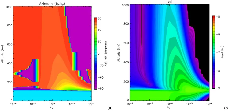
So far we have only considered varying the wavenumber in the east-west direction, holdingkx≈0. Figure 9 shows the effect on the polarisation azimuth for different values ofkx whileky ≈ 0, computed from the numerical model. Com-paring this with Fig. 5, the azimuth rotation is similar to the

ky dependent case. However, the amount of field aligned ULF wave magnetic perturbation,|b|||is quite different. For small wavenumbers,|b||| is significantly reduced above the ionosphere E-region, while in the atmosphere,|b|||is large. Using the analytic model, the conversion coefficient,|AF|

(shear Alfv’en to compressional mode) is 0.05, which ac-counts for the small compressional mode amplitude above the ionosphere E-region. The reflection coeffecient for the shear Alfv´en mode,|AA|=0.85. Therefore, the angle of ar-rival (changing the relative magnitudes ofkx andky) has a significant effect on the amount of compressional mode that appears just above the ionosphere. In the atmosphere, theb|| signal comes from the magnetospherebxcontribution due to the obliqueB0. This may be understood from Fig. 8 where

the fields are shown for the case wherekx≈0. Forky≈0, the

bx andbz components of the shear Alfv´en mode reduce in magnitude to theby level in Fig. 8 while theby component increases to the magnitude ofbxin Fig. 8. The shear Alfv´en mode has most of its amplitude inby forky≈0. Therefore, the compressional mode that appears has similar magnitude inbzbutbxis large forky≈0 whilebyis large forkx≈0. The projection of the largebx onto theB0direction forky≈0 is the source of the larger field aligned component in the atmo-sphere.

Polarisation azimuth rotation for ULF waves that en-counter the ionosphere has historically addressed the shear Alfv´en mode with its associated field aligned current. Both wave modes are usually involved when computing the polari-sation azimuth frombxandbynear the ionosphere. Does the compressional mode exhibit similar behavior? The structure

Fig. 8. Separation of the ULF magnetic wave fields using the analytical model of Sciffer et al. (2004). The parameters are the same as Fig. 7 but withky=4×10−6m−1. Left-hand-panels show the magnitude of the respective wave fields while the right-hand-panels show the phasing.

of the compressional mode for ideal MHD conditions is shown in Fig. 10 forky=0. The mode has perturbation cur-rent perpendicular to both band k, and parallel to e. For

ky≈0, the shear Alfv´en mode is confined tobyand the com-pressional mode tobx andbz. Hence we can see that for a compressional mode in the magnetosphere withky=0,∇×b is in the y direction. In the neutral atmosphere, the wave magnetic field must either be zero or aligned alongk, which is in thexzplane. If conversion to the shear Alfv´en mode is zero, the rotation of the magnetic wave field is confined to the xzplane. Therefore, there is no NDR for the com-pressional mode in thexyandyzplanes. The compressional mode reflection coefficient is ≈−1 so the incident and re-flectedbzcomponents cancel while the incident and reflected

(a) (b)

Fig. 9. The(a)polarisation azimuth computed from thebxandbyULF wave fields and(b)the field aligned component of the ULF wave field for a frequency of 16 mHz, dip angleI=70◦for solar maximum parameters. The east-west wavenumber,ky=1×10−10m−1.

x

z, B₀ v

j b

e

k _k

y=0

Fig. 10.The structure of a compressional ULF wave mode for ideal MHD andky=0 (Cross, 1988).

azimuth change in theyzplane. For a mix of incident, prop-agating wave modes,kz,f is larger thankxto ensure the com-pressional mode propagates and a NDR appears in the yz

plane.

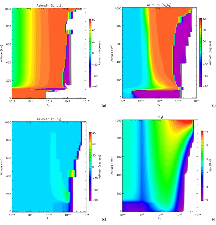
A polarisation azimuth rotation can appear for the incident compressional mode case ifkvaries in theydirection which is perpendicular to the plane ofB0. A representative example

is shown in Fig. 11 where the dip angle is 70◦_,k

x=1×10−10 for a wave frequency of 16 mHz. The polarisation azimuth in the atmosphere compared with that above the ionosphere E-region (120 km) changes in thexyandxzplanes for smallky. Forky=4×10−8m−1 the incident compressional mode has field perturbations in all three components withbx≈by and

bz≈0.1bx. The compressional mode reflection coefficient,

|F F|≈0.1 while the compressional to shear Alfv´en conver-sion,|F A|≈0.8. The resulting magnetic fields of the wave in the atmosphere are bx≈bz with by≈100bx. Therefore,

the reduction inbxamplitude from the magnetosphere to the atmosphere results in polaristion azimuth rotation in thexy

andxzplanes as seen in Fig. 11.

Compressional mode wave energy is generally thought to enter the magnetosphere from external sources such as the Kelvin-Helmholtz instability in the vicinity of the magne-topause (Southwood, 1968) or upstream ion-cyclotron wave generation (Yumoto, 1985). Propagation of compressional mode energy from the magnetosphere to the ionosphere and ground is hampered by wave propagation cutoffs in the mag-netosphere (Zhu and Kivelson, 1989). This does not neces-sarily preclude the existence of propagating compressional mode waves around 1000 km altitude. Compressional mode energy may “tunnel” and appear as a propagating mode in the inner magnetosphere (Allan et al., 1986; Waters et al., 2000). Furthermore, an incident shear Alfv´en wave that mode con-verts in the ionosphere may produce an upward propagating compressional mode as described in the context of Figs 4, 5, 7, and 9. If the compressional mode does not decay suffi-ciently with increasing altitude and appears in the top side ionosphere, then an azimuth rotation in the vertical plane does occur but is not necessarily 90◦_.

6 Conclusions

The polarisation azimuth rotation of ULF waves in the horizontal plane (bx,by) from the magnetosphere through to the atmosphere does occur for oblique B0. However,

(a) (b)

(c) (d)

Fig. 11. Polarisation azimuths for an incident compresional (fast) mode. The ULF frequency was 16 mHz, the dip angle,I=70◦and solar maximum conditions. Wavenumbers arekx=10−10m−1andkyvarying between 10−8m−1and 10−4m−1.(a)Polarisation azimuth forbx andby,(b)polarisation azimuth forbx andbz and(c)polarisation azimuth forbyandbz,(d) the amplitude of the field aligned (compressional) component of the ULF wave magnetic field.

small altitude range, close to the ionospheric E-region. If the compressional energy propagates or has a largeefolding distance, then the polarisation azimuth in the top side iono-sphere or magnetoiono-sphere compared with the atmoiono-sphere can be any value, as seen in the left portion of Fig. 7d. These conditions may be satisfied for low latitudes and small m

azimuth rotation effect but in the vertical plane, involving

bx,bzfor ky≈0. Forkx≈0, the compressional wave energy appears in all 3 spatial components. However, in all cases, as was pointed out by Southwood and Hughes (1983), the

∇×bchanges from non-zero in the magnetosphere to zero in the atmosphere. This may or may not be manifested as a rotation of polarisation azimuth computed from the wave magnetic field components.

The numerical model described in this paper assumes a 1-D, horizontally uniform ionosphere, an approximation used in previous studies. We have focussed on the effects introduced by different magnetic field dip angles with latitude. The effect of the dip angle is introduced into the model via the conductivity tensor, σ¯. Since ULF wave spatial scale sizes may be up to thousands of km, the as-sumption of horizontal uniformity inσ¯ over these distances is more reasonable for the azimuthal direction (provided the dawn and dusk longitudes are avoided) compared with the latitudinal direction. In order to fully quantify the validity of these assumptions, the results need to be compared with those from a higher dimensional model, a task presently underway.

Appendix

The direct, Pedersen and Hall conductivities of an ionised gas can be derived from equations of motion of the plasma. They may be expressed as,

σ0= 1

B0

X

i

nii

¯

vi

|qi| (A1)

σ1= 1

B0

X

i

ni2_ivi

¯

v2_i +2_i|qi| (A2) σ2= −

1

B0

X

i

2_iqi

¯

v_i2+2_i|qi| (A3)

whereni,i, andqi are the number density, gyrofrequency and charge of theith particle species.v¯i=vi−iωfor the col-lision frequency, vi, and the characteristic frequency, ω of the disturbance.B0is the magnitude of the background mag-netic field. The collision frequencies may be calculated from the number densities of the given species together with the temperature, mean molecular mass and density of the neutral components (Kelley, 1989). The values required for these calculations were obtained from the IRI95 and MSISE90 models. The IGRF model was used for magnetic field values as well as dip angle for a particular locality. The values for the conductivities were calculated in 2 km increments from 80 km to 1000 km.

The values below 80 km (or where the IRI and MSIS model had no data) were reduced with decreasing altitude, starting with the lowest altitude value. The direct and Pedersen conductivities were decreased using an efolding distance of 6 km in the original model of Hughes (1974).

In general, the direct and Pedersen conductivities were chosen to decrease with an e folding distance of 3 km which produced a smaller conductivity near the ground (≈2×10−14S/m). The Hall conductivity has an efolding distance set to 1 km (e.g. Zhang and Cole, 1994).

Acknowledgements. This work was supported by grants from the Australian Research Council, the University of Newcastle and the Cooperative Research Centre for Satellite Systems. The authors wish to thank P. Ponomarenko for helpful discussions.

Topical Editor M. Pinnock thanks W. J. Hughes and another referee for their help in evaluating this paper.

References

Allan, W., Poulter, E., and White, S.: Hydromagnetic wave cou-pling in the magnetosphere- Plasmapause effects on impulse-excited resonances, Planet. Space Sci., 34, 1189–1200, 1986. Cross, R.: An introduction to Alfv´en waves, Addison Wesley,

Mas-sachusetts, 1988.

Hedin, A. E.: A revised thermospheric model based on mass spec-trometer and incoherent scatter data: MSIS-83, J. Geophys. Res., 88, 10 170–10 188, 1991.

Hughes, W. J.: The effect of the atmosphere and ionosphere on long period magnetospheric micropulsations, Planet. Space Sci., 22, 1157–1172, 1974.

Hughes, W. J. and Southwood, D.: The screening of micropulsation signals by the atmosphere and ionosphere, J. Geophys. Res., 81, 3234–3240, 1976.

Kelley, M. C.: The Earth’s Ionosphere – Plasma Physics and Elec-trodynamics., Academic Press Inc., 1989.

Olson, J. V. and Rostoker, G.: Longitudional phase variation of Pc 4-5 micropulsations., J. Geophys. Res., 83, 2481–2488, 1978. Pitteway, M. L. V.: The numerical calculation of wave fields,

re-flection coefficients and polarizations for long radio waves in the lower ionosphere., Roy, Soc. Phil. Trans., 257, 219–239, 1965. Poole, A. W. V., Sutcliffe, P. R., and Walker, A. D. M.: The

rela-tionship between ULF geomagnetic pulsations and ionospheric doppler oscillations: Derivation of a model., J. Geophys. Res., 93, 14 656–14 664, 1988.

Sciffer, M. D. and Waters, C. L.: Propagation of ULF waves through the ionosphere: Analytic solutions for oblique magnetic fields, J. Geophys. Res., 107, 1297–1311, 2002.

Sciffer, M. D., Waters, C. L., and Menk, F. W.: Propagation of ULF waves through the ionosphere: Inductive effect for oblique magnetic fields, Ann. Geophys., 22, 1155–1169, 2004,

SRef-ID: 1432-0576/ag/2004-22-1155.

Southwood, D. J.: The hydromagnetic stability of the magneto-spheric boundary, Planet. Space Sci., 16, 587–605, 1968. Southwood, D. J. and Hughes, W. J.: Theory of hydromagnetic

waves in the magnetosphere, Space Sci. Rev., 35, 301–366, 1983. Stix, T. H.: The theory of plasma waves., McGraw-Hill, New York,

1962.

Waters, C. L., Harrold, B. G., Menk, F. W., Samson, J. C., and Fraser, B. J.: Field line resonances and waveguide modes at low latitudes: 2. A model, J. Geophys. Res., 105, 7763–7774, 2000. Yoshikawa, A. and Itonaga, M.: The nature of reflection and mode

Yoshikawa, A., Obana, Y., Shinohara, M., Itonaga, M., and Yumoto, K.: Hall-induced inductive shielding effect on geomagnetic pul-sations, Geophys. Res. Lett., 9, 8, doi:10.1029/2001GL013610, 2002.

Yumoto, K.: Low-Frequency upstream wave as a probable source of low-latitude Pc3-4 magnetic pulsations, Planet. Space Sci., 33, 239–249, 1985.

Zhang, D. Y. and Cole, K. D.: Some aspects of ULF electromag-netic wave relations in a stratified ionosphere by the method of boundary value problem., J. Atmos. Terr. Phys., 56, 681–690, 1994.

Zhang, D. Y. and Cole, K. D.: Formulation and computation of hydromagnetic wave penetration into the equatorial ionosphere and atmosphere, J. Atmos. Terr. Phys., 57, 813–819, 1995. Zhu, X. and Kivelson, M. G.: Global mode ULF pulsation in a