The Beta Truncated Pareto Distribution
Lourenzutti R.a
, Duarte D.a∗
, Castellares F.a
and Azevedo M.a
Universidade Federal de Minas Gerais,Belo Horizonte, MG, Brazil;
The Pareto distribution is widely used to modelling a diverse range of phenomena. Many transformations and generalization of the Pareto law distribution have been proposed in order to get more flexible models. In fact, these generalizations are very common in literature. Recently a new family of distribution, called Beta Generated distribution, was proposed. This family presents itself as a very flexible family, capable of modelling symmetric and skewed data. In this work we apply the beta transformation to the truncated Pareto distribution. We analyse some of its properties and apply it to real data. For estimation we the minimum distance method. This new distribution, called Beta truncated Pareto, proved to be a very flexible.
Keywords:power law; tuncated Pareto distribution; beta generated family; minimum distance method;
1. Introduction
In 1896, Vilfredo Pareto noticed that the income distribution "follows a power law
behavior", i.e., the pdf of income has the form f(x)∝x−α−1 [see 1]. Later, it was
found that the power law distribution is present in a diverse range of phenomena, as for instance, the sizes of earthquakes [2], solar flares [3][also, see 4], the frequency of use of words in any human language [5], the frequency of occurrence of personal names in most cultures [6], the numbers of papers that scientists write [7], the number of citations received by papers [8] and hydrological data [9]. Also, some recent works about the power law distribution (also known as Pareto distribution) corroborate with the hypothesis made by Pareto [see 10–12].
Many extensions of the Pareto distribution were proposed in literature. For ex-ample, the transformed Pareto distribution [13, p. 193], the truncated Pareto dis-tribution (TPD) [14, 15], the double Pareto disdis-tribution [16], the double Pareto-lognormal distribution [17] and the Generalized Pareto distribution (GPD) [see 18, 19]. The TPD and GPD are ones of the most important extensions of the Pareto distribution.
In [15], the Pareto and truncated Pareto distributions were applied to astro-physics data and they concluded that, in general, the truncated Pareto distribution performs better than the usual Pareto distribution. If the difference between the maximum and minimum values of the sample is high, then there is no real difference between the two distributions.
gener-alized family of distributions. Then, a statistical analysis of the parameters can indicate properly whether one of the simpler families is better fitted to the data or if the new proposed distribution provides a more appropriate solution.
Recently, a new family of distributions, generated from the Beta distribution has been proposed by [25]. In that proposal the Beta distribution was used to generalize the Normal family. Later, [26] proposed, in a general fashion, the Beta Generated family. The Pareto family was generalized through the same methodology by [27]. Many properties of the Beta Generated family are shown in [28]. It is becoming evident that the Beta Generated family is a very flexible family of distributions.
Motivated by the works of [14, 15] and [27], we propose the Beta truncated Pareto distribution. We explore some of its characteristics and we compare its performance to the Beta Pareto distribution and other distributions.
This paper is organized as follows. Section 2 introduces the Beta truncated Pareto distribution and presents some of its properties. Section 3 provides inferential re-sults. Section 4 shows an application of BTPD to a real data and Section 5 presents concluding remarks.
2. The Beta Generated Family and the Beta truncated Pareto
LetZ and Y be two random variables, where Z ∼Beta(α, β) and Y has cdf FY.
DefineX=FY−1(Z). Then, X has probability density function (pdf) given by
fX(x|α, β,p) = 1
B(α, β)fY(x) [FY(x)] α−1[1
−FY(x)]β−1 (1)
and cumulative distribution function (cdf) given by
FX(x|α, β,p) =
BFY(x)(α, β)
B(α, β) , (2)
whereB(a, b)is the beta function,pis a parameter vector associated withFY, and
Bx(a, b) =
Rx
0 ua
−1(1−u)b−1du, 0< x <1, is the incomplete beta function.
In this case, FX represents a beta generated distribution with parent
distribu-tion FY. Note that if α and β are integers then we have the distribution of order
statistics. Furthermore, if α = 1 and β = 1, the Equation 1 becomes the parent
density.
Now make Y ∼ T P(θ, λ, k), where T P means truncated Pareto distribution.
ThenY has cdf given by
FY(y) =
1−(θy)k
1−(θλ)k, 0< θ < λ,k >0and θ < y, < λ (3)
and pdf given by
fY(y) =
kθky−(k+1)
1−(λθ)k , 0< θ < λand θ < y < λ. (4)
Define a new variable X as X =F−1
Y (Z) = θ
n
1−Zh1−(θ/λ)kio−1/k. Then,
fX(x) = 1
B(α, β)
kθkx−(k+1)
1−(θλ)k
"
1−(θx)k 1−(λθ)k
#α−1"
1− 1−( θ x)k 1−(θλ)k
#β−1
, θ < x < λ. (5)
In this case, it can be said that X follows a Beta truncated Pareto
distribu-tion (BTPD) with parameters α, β, θ, λ and k, hereafter defined as X ∼
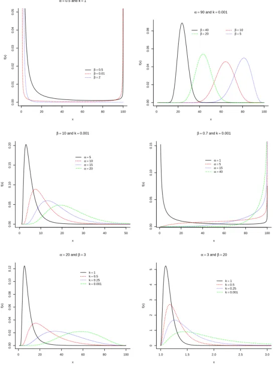
BT P(α, β, θ, λ, k). As shown in Figure 1, the α and β parameters are related to
the shape of the distribution whereas the parameterkis related to the scale of the
distribution, but also has effect on the shape.
The cdf of X is obtained directly from Equation 2, shown as follows,
FX(x) =
BFY(x)(α, β) B(α, β)
=I(x)(θ,λ)× 1
B(α, β) ∞
X
i=0
(1−β)i
i!(α+i)
"
1− xθk
1− λθk #α+i
+I(x)[λ,∞)
where(x)n=x(x+ 1)(x+ 2). . .(x+n−1).
Now consider the Pareto distribution. The pdf and cdf are given, respectively, by
h(y) = k
θ
θ y
k+1
and H(y) = 1−
θ y
k
, θ < y <∞.
Letc(k, θ, λ) :=c(k) =h1− λθki−1
. Then we can rewrite (3) and (4) as
fy(y) =c(k)h(y) and FY(y) =c(k)H(y), θ < y < λ.
By Equation 1, the BTPD density is
fX(x) = 1
B(α, β)fY(x) [FY(x)] α−1[1
−FY(x)]β−1
= 1
B(α, β)c
α(k)h(x) [H(x)]α−1[1
−c(k)H(x)]β−1.
As the term|c(k)H(x)|is strictly less than 1 in the intervalθ < x < λ, then
fX(x) = ∞
X
i=0
(−1)i β−1
i
B(α, β) [c(k)]
ButH(x) can be rewritten as H(x) =P∞
j=0(−1)j α+i
−1
j
θ
x
kj
. Therefrom
fX(x) = ∞
X
i=0
∞
X
j=0
(−1)i+j β−i1 α+i−1
j
B(α, β) [c(k)] α+ik
θ
θ x
k(j+1)+1
= ∞
X
i=0
∞
X
j=0
A(i, j)c(k(j+ 1))k(j+ 1)
θ
θ x
k(j+1)+1
where
A(i, j) = (−1)
i+j β−1
i
α+i−1
j
(j+ 1)B(α, β)
[c(k)]α+i
c(k(j+ 1)).
It shows that the Beta truncated Pareto distribution is an infinite linear
combina-tion of truncated Pareto distribucombina-tion with parametersk(j+ 1), θ and λand with
sum coefficientsA(i, j).
2.1. Special Cases
Three different families of distributions are identified as special cases from the BTPD. These families are already proposed in the literature and they are shown next.
(1) If α = 1 and β = 1 then the density shown in Equation 5 becomes the
density of a truncated Pareto random variable.
(2) The Beta Pareto family proposed by [27] is also a special case. In this case its density is given by
f(x) = k
θ·B(α, β)
"
1−
θ x
k#α−1
θ x
k·β+1
, wherex > θ, (α, β, θ, k)>0.
(6)
This density represents a limiting density of BTPD when λ→ ∞.
(3) If α = 1, β = 1 and λ→ ∞ then the Pareto family is a limiting family of
BTPD family.
2.2. Limit Behavior
The behavior of BTPD whenx→θandx→λchanges according to parametersα
andβ. The limits of BTPD in both cases are presented next.
Proposition 2.1:
lim
x→θfX(x) =
∞ , 0< α <1 βk
θh1−(θ λ)
ki , α= 1
0 , α >1
0 20 40 60 80 100
0.00
0.01
0.02
0.03
0.04
0.05
α =0.5 and k=1
x
f(x)
β =0.5
β =0.01
β =2
0 20 40 60 80 100
0.00
0.02
0.04
0.06
0.08
α =90 and k=0.001
x
f(x)
β =40
β =20
β =10
β =5
0 10 20 30 40 50
0.00
0.05
0.10
0.15
0.20
β =10 and k=0.001
x
f(x)
α =5
α =10
α =15
α =20
0 20 40 60 80 100
0.00
0.05
0.10
0.15
β =0.7 and k=0.001
x
f(x)
α =1
α =5
α =15
α =40
0 20 40 60 80 100
0.00
0.02
0.04
0.06
0.08
0.10
0.12
α =20 and β =3
x
f(x)
k=1 k=0.5 k=0.25 k=0.001
1.0 1.5 2.0 2.5 3.0
0
1
2
3
4
5
α =3 and β =20
x
f(x)
k=1 k=0.5 k=0.25 k=0.001
Figure 1. Density function forθ= 1,λ= 100and some values deα,βandk.
lim
x→λfX(x) =
∞ , 0< β <1 αkθk
λk+1h1−(θ λ)
ki , β= 1
0 , β >1
(8)
Proof : Obtained from the pdf presented in Equation 5
It is worth noting in Equation 7 that if x→ θthen the parameter α defines the
limit behavior of the density. If x → λ then the parameter β controls the limit
2.3. Moment Generating function of BTPD
In this section the Moment Generating function for the BTPD is presented. We will make use of the following result.
Lemma 2.2: The power serie P∞i=0 (r/ki!)iui
h
1− θλkii
, is uniformly convergent in the interval[0,1].
Proof : The radius of convergence, l, of a power serie,P
anxn, is given by
l−1= lim
i→∞sup√iai. In this case,
l−1 = lim
i→∞sup i
v u u
t(r/k)i
i! " 1− θ λ
k#i
= " 1− θ λ k# lim i→∞sup
i
r
(r/k)i
i!
But limi→∞sup
i
q
(r/k)i
i! is the radius of convergence of the well known power
serie P∞
i=0(−1)i r/ki
ui = (1 − u)r/k. Thus limi→∞sup
i
q
(r/k)i
i! = 1. Thereof
l = h1− θλki−1
. So, since l > 1, the closed interval [0,1] ⊂ (−l, l). Therefore
the serie is uniformly convergent in the interval[0,1].
The moments of BTPD are presented in the following proposition.
Proposition 2.3: The moments of the BTPD are given by
E[Xr] = θ r
B(α, β) ∞
X
i=0
(r/k)i
i! " 1− θ λ
k#i
B(α+i, β) (9)
Proof : : Using the transformation u=FY(x), it can be shown that
E[Xr] =
Z λ
θ 1
B(α, β)
"
1− θxk
1− θλk #α−1"
1−1− θ x
k
1− λθk #β−1
kθk xk+1−r
1− θλkdx
= θ r
B(α, β)
Z 1
0
uα−1(1−u)β−1
(
1−u
"
1−
θ λ
k#)−r/k
du
= θ r
B(α, β)
Z 1
0
uα−1(1−u)β−1
∞
X
i=0
(r/k)i
i! u i " 1− θ λ
k#i
du
= θ r
B(α, β) ∞
X
i=0
(r/k)i
i! " 1− θ λ
k#i
B(α+i, β)
Note that Rλ
θ xrf(x)dx ≤
Rλ
θ λrf(x)dx ≤λr. So all the moments of the BTPD
are finite.
Lemma 2.4: The moment generating function of BTPD is
M(t) = 1
B(α, β) ∞ X r=0 ∞ X j=0
(tθ)r
r!
(r/k)j
j! " 1− θ λ
k#j
B(α+j, β)
Proof : SinceP∞ r=0t
r
r!xrf(x)converges and each term is integrable for alltclose to
0, then we can rewrite the moment generating function asM(t) =P∞
r=0t
r
r!E[Xr].
By replacingE[Xr]by the right side of Equation 9 the desired result is obtained.
2.4. Mean Deviations
Consider the two following mean deviation:
i) Mean Deviation from the mean:D(µ) =E[|X−E(X)|].
ii) Mean Deviation from the median:D(M) =E[|X−M|], whereM is the median.
In general, the mean deviation from the mean is used for symmetric distributions while the mean deviation from the median is used for skewed distributions. For the BTPD density we have the following property.
Proposition 2.5: The mean deviation from the mean and the mean deviation
from the median for the Beta truncated Pareto density are given, respectively, by
i) D(µ) = 2µF(µ)−2B(α,βθ )P∞
i=0 (1/k)i
i!
h
1− θλkii
BFY(E[X])(α+i, β).
ii) D(M) =µ−2B(α,βθ )P∞
i=0 (1/k)i
i!
h
1− λθkii
BFY(M)(α+i, β).
Proof : Consider that
D(µ) =
Z λ
θ |
x−µ|f(x)dx
= 2
Z µ
θ
(µ−x)f(x)dx+
Z λ
θ
(x−µ)f(x)dx
= 2µF(µ)−2
Z µ
θ
xf(x)dx,
and, in a similar way,
D(M) =µ−2
Z M
θ
xf(x)dx.
Using the transformationu=FY(x) and Lemma 2.2, then
Z c
θ
xf(x)dx= θ
B(α, β)
Z FY(c)
0
uα−1(1−u)β−1
∞
X
i=0
(1/k)i
i! u i " 1− θ λ
k#i
du
= θ
B(α, β) ∞
X
i=0
(1/k)i
i! " 1− θ λ
k#iZ FY(c)
0
uα+i−1(1−u)β−1du
= θ
B(α, β) ∞
X
i=0
(1/k)i
i! " 1− θ λ
k#i
Assuming thatc=µ andc=M, the desired results are obtained.
2.5. Lorenz’s Curve
The Lorenz’s curve was proposed by [29] to study the distribution of income and wealth within the population. The Lorenz’s curve was used to describe the
propor-tion of populapropor-tion risk that falls below thep-th quantile of risk in [30].
The Lorenz’s curve is defined as,
L(p) = 1
E[X]
Z FX−1(p)
0
tf(t)dt, 0≤p≤1 (11)
In the BTPD case we have the following.
Lemma 2.6: The Lorenz’s curve for the BTPD is given by
L(p) = θ
E[X]B(α, β) ∞
X
i=0
(1/k)i
i!
"
1−
θ λ
k#i
BFY(FX−1(p))(α+i, β) (12)
Proof : Result obtained by making c=F−1
X (p) in Equation 10.
2.6. Entropies
In this section we present two entropy measures: the Renyi entropy and the Shan-non’s entropy.
2.6.1. Rényi’s entropy
Consider the Rényi’s entropy, defined as
IR(ǫ, f) = 1 1−ǫlog
Z
❘f
ǫ(x)dx
. (13)
then, for the BTPD, we have the following proposition
Proposition 2.7 Rényi’s entropy: The Rényi’s entropy for the BTPD is given by
IR(ǫ, f) = log
θ k
−1 ǫ
−ǫlogB(α, β) +
+ 1 1−ǫlog
∞
X
i=0
(ǫ−1)(k+1)
k
i
i!
"
1−
θ λ
k#i+1−ǫ
B(α1, β1)
(14)
Proof : Applying the transformation u=FY(x), it can be shown that
Z
❘f
ǫ(x)xdx=
Z λ
θ 1
Bǫ(α, β)
"
1− xθk
1− λθk
#ǫ(α−1)"
1−1− θ x
k
1− θλk
#ǫ(β−1)" kθk xk+1 1− θλk
#ǫ
dx
=
Z 1
0
1
Bǫ(α, β)u
ǫ(α−1)(1−u)ǫ(β−1)
" kθk xk+1 1− λθk
#ǫ−1
du
= k
ǫ−1θ1−ǫ
Bǫ(α, β)h1− θ λ
kiǫ−1 ×
×
Z 1
0
uǫ(α−1)(1−u)ǫ(β−1)
(
1−u
"
1−
θ λ
k#)(k+1)(ǫ−1)/k
du
= k
ǫ−1θ1−ǫ
Bǫ(α, β)h1− θ λ
kiǫ−1 ×
× ∞
X
i=0
(−1)i
(ǫ−1)(k+1)
k
i
"
1−
θ λ
k#i
B(α1, β1)
then applying Equation 13, Equation 14 is obtained. Note that we made use of the
Lemma 2.2 here.
2.6.2. Shannon’s entropy
The Shannon’s entropy [see 28, and references therein] is defined as
ISh(f) =−
Z
❘f(x) logf(x)dx.
Was proved by [28] that for the Beta generated family the Shannon’s entropy is given by
ISh(f) = logB(α, β)−(α−1) [ψ(α)−ψ(α+β)]−(β−1) [ψ(β)−ψ(α+β)]− −E
logfY FY−1(Z). (15)
We present the following result for BTPD.
Lemma 2.8: For the BTPD and following Equation 15, it can be shown that
E
logfY FY−1(Y)= log
k θ −log
h
1−(θ/λ)ki− ∞
X
i=1
h
1−(θ/λ)kii
iB(α, β) B(α+i, β).
Proof :
E
logfY FY−1(Y)= logk+klogθ−log
h
1−(θ/λ)ki−(k+ 1) logθ+
+k+ 1
k E
h
and
Ehlogn1−Y h1−(θ/λ)kioi=
Z 1
0
logn1−Y h1−(θ/λ)kio 1
B(α, β)y
α−1(1−y)β−1dy
=
Z 1
0
∞
X
i=1
yih1−(θ/λ)kii
i
1
B(α, β)y
α−1(1−y)β−1dy
=− ∞
X
i=1
h
1−(θ/λ)kii
iB(α, β) B(α+i, β)
2.7. Hazard Rate Function
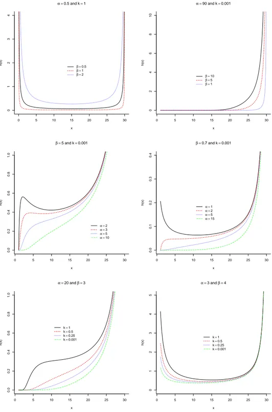
It was showed in Figure 1 some of different forms that the density of BTPD is capable to assume. It is not different for the Hazard Rate function as it is shown here.
Lemma 2.9: For BTPD, the Hazard Rate function has the form
h(x) = f(x) 1−F(x)
=
1−(θx) k
1−(θ λ)
k
α−1
1− 1−( θ x)
k
1−(θ λ)
k
β−1
kθk x−k−1 1−(θ
λ) k
B(α, β)−BFY(x)(α, β)
(16)
The limit of the Hazard Rate function is given by
lim
x→θh(x) =
∞ , 0< α <1 βk
θh1−(θλ)
ki , α= 1
0 , α >1
(17)
lim
x→λh(x) = ∞ (18)
Some forms of Hazard Rate function of BTPD are shown in Figure 2.
3. Inference Issues About the BTPD
The maximum likelihood method for point estimation is the most used method in literature. Alternatively, estimates for the parameters can be found using the method of moments. In this case, estimates are obtained by solving the following non-linear equations
1
n
n
X
i=1
Xr= θ
r
B(α, β) ∞
X
i=0
(r/k)i
i!
"
1−
θ λ
k#i
0 5 10 15 20 25 30
0
1
2
3
4
α =0.5 and k=1
x
h(x) β =
0.5
β =1
β =2
0 5 10 15 20 25 30
0
2
4
6
8
10
α =90 and k=0.001
x
h(x)
β =10
β =5
β =1
0 5 10 15 20 25 30
0.0
0.2
0.4
0.6
0.8
1.0
β =5 and k=0.001
x
h(x)
α =2
α =3
α =5
α =10
0 5 10 15 20 25 30
0.0
0.1
0.2
0.3
0.4
β =0.7 and k=0.001
x
h(x) α =
1
α =2
α =5
α =15
0 5 10 15 20 25 30
0.0
0.2
0.4
0.6
0.8
1.0
α =20 and β =3
x
h(x)
k=1 k=0.5 k=0.25 k=0.001
0 5 10 15 20 25 30
0
1
2
3
4
5
α =3 and β =4
x
h(x)
k=1 k=0.5 k=0.25 k=0.001
Figure 2. Hazard Hate function forθ= 0.01,λ= 30and some values deα,βandk.
A modified method of moments was proposed by [28]. Nevertheless, the method of moments is not a very reliable approach and it is usually used as initial estimative for the maximum likelihood approach. The main advantage of maximum likelihood estimators is that, under some regularity conditions, they have desirable properties. However, these conditions are not satisfied here.
behind the method is minimizing the distance between the empirical cdf and the theoritical cdf, this method was called estimation by the minimum distance method (MDM) [see 31, and references therein]. Also, [32] shows the consistency and found the asymptotic distribution of the estimator of minimum distance (MDE). Through a simulation study of many different MDM statistics, [33] analysed the perform of MDE for generalized Pareto distribution and concluded that MDE had a very good performance. Thus, we also apply this method to estimate the parameters of the BTPD.
The BTPD hasfX(x)>0, only ifθ < x < λ. Estimates forθandλare:θˆ=X(1)
and ˆλ = X(n), where X(1) is the first order statistic and X(n) is the last one.
The estimates for α, β and k are chosen so that the maximum distance between
the empirical cdf and the BTPD cdf (called by Kolmogorov distance in [33]) is minimized, i.e.,
( ˆα,β,ˆ kˆ) = arg min α,β,k1max≤i≤n
Fn(xi)−FX
xi
ˆ
θ,λˆ
(20)
whereFn(x) = n1Pin=1I(Xi≤x).
Proposition 3.1: The estimators θˆ=X(1) and λˆ=X(n) are consistent.
Proof : For any ǫ >0we have
Ph
ˆ
θ−θ
< ǫ
i
=P
θ−ǫ < X(1) < θ+ǫ
=FX(1)(θ+ǫ)−FX(1)(θ−ǫ)
= [1−FX(θ−ǫ)]n−[1−FX(θ+ǫ)]n
Since the support offX is in the interval(θ, λ), we have that FX(θ−ǫ) = 0 and
FX(θ+ǫ)>0. Thuslimn→∞P
h θˆ−θ
< ǫ
i
= 1. In an analogous way we have,
lim n→∞P
h ˆλ−λ
< ǫ
i
= lim
n→∞{[FX(λ+ǫ)] n
−[FX(λ−ǫ)]n} = 1
4. Applications
In order to illustrate the use and the performance of the BTPD proposal, we ap-plied the proposed distribution to real data and we compared the results with the following distributions:
(i) The truncated Pareto distribution (TPD).
The GP distribution has the following pdf
f(x) = 1
a
1−kx
a
(1−k)/k
0< xifk≤0
0< x < a/kif k >0
(iii) The Weibull distribution with three parameters (TPWD). The density of this distribution is given by
f(x) =γb−γ(x−a)−γ−1exp
−
x−a b
γ
, x > a γ, b >0.
(iv) The Beta Pareto distribution (BPD). The density of this distribution is presented in Equation 6.
In order to compare the models we will use the K-S statistic given by
KS(Fest) = max
1≤i≤n|Fn(xi)−Fest(xi)|, (21)
whereFest is the model’s c.d.f using the estimated parameters. We will also provide
the absolute mean distance statistic given by
D(Fest) = 1
n
n
X
i=1
|Fn(xi)−Fest(xi)| (22)
4.1. Castelo River
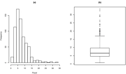
The data consist of 684 maximum values of monthly flood rates of the Castelo River, in Brazil, and it is available online (hidroweb.ana.gov.br). Table 1 shows summary statistics of the data. The Figure 3 shows the histogram and box plot of the data. It is worth noticing the strong asymmetry of the distribution of the data to the right. This behavior is quite common in hydrology data.
Table 1. Descriptive statistics of maximum monthly flood rate of Castelo River.
Min. 1st Qu. Median Mean 3rd Qu. Max. Std. Dev.
0.740 4.602 6.555 7.704 9.678 33.4 4.6178
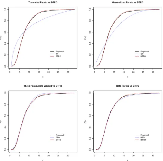
The Table 2 and Figure 4 present the results obtained by the MDE. The K-S and D statistics present very high values for TPD and GPD, suggesting a quite poor adjust to the data. Despite this improvement, the KS-statistic remained very high. The K-S test rejected both, TPD and GPD distributions, as appropriate models. For the TPWD, the D and K-S statistics are better than for the TPD and GPD. The K-S test now does not reject the TPWD as an appropriate model at 5% of significance.
(a)
Flood
Frequency
0 5 10 15 20 25 30 35
0
50
100
150 ●
●
● ● ● ●
● ● ● ● ● ● ●
● ● ● ● ●
● ●
● ● ● ● ● ● ●
0
5
10
15
20
25
30
(b)
Figure 3. Castelo River flood: (a) Histogram (b) Box-Plot.
Table 2. KS Estimative of parameters and KS and D statistics.
TPD GPD TPWD BPD BTPD
ˆ
k= 10312; ˆa= 12.0612; ˆa= 0.74; αˆ = 15.79; αˆ = 9.8228;
Estimatives ˆk= 0.3397; ˆb= 7.4360; βˆ= 64.14; βˆ= 3.9035;
ˆ
γ = 1.8658; ˆk= 0.1; ˆk= 0.347;
KS 0.3005 0.1586 0.0399 0.0276 0.0182
D 0.1438 0.0995 0.0207 0.0116 0.0082
5. Conclusion
In this work a new family of distribution called Beta truncated Pareto distribution was introduced and some of its properties were analysed. The BTPD proved to be a very flexible model with many different forms for its density (as it can be seen in Figure 1). Also, the BTPD includes some other families that were already proposed in literature. For the parameters estimation we used the minimum distance method. In order to evaluate the BTPD performance we applied the BTPD to real data. The TPD and GPD a very poor fit. The TPWD had a good fit was not rejected by the KS test. The BTPD and BPD have the best fit to the data with a small advantage for BTPD. They both followed the empirical distribution very closely when the MDE were applied.
Due to the fact that the BTPD has two more paramaters than the TPWD, one could be favorable to TPWD arguing that the difference between the adjust obtained by the TPWD and the adjust obtained by the BTPD is small. That is not so clear. Despite the KS test does not reject either, we have a sample size of
684 which makes the cost of the two additional parameters not so high. Beyond
that the K-S statistic for the BTPD is less than a half of the KS statistic for the TPWD.
References
[1] B. C. Arnold,Pareto Distribution, Fairland: International Co-operative Publishing House (1983). [2] B. Gutenberg and R. F. Richter,Frequency of earthquakes in california., Bulletin of the Seismological
Society of America (1944).
0 5 10 15 20 25 30
0.0
0.2
0.4
0.6
0.8
1.0
Truncated Pareto vs BTPD
x
F(x)
Empirical TP BTPD
0 5 10 15 20 25 30
0.0
0.2
0.4
0.6
0.8
1.0
Generalized Pareto vs BTPD
x
F(x)
Empirical GP BTPD
0 5 10 15 20 25 30
0.0
0.2
0.4
0.6
0.8
1.0
Three Parameters Weibull vs BTPD
x
F(x)
Empirical TPW BPTD
0 5 10 15 20 25 30
0.0
0.2
0.4
0.6
0.8
1.0
Beta Pareto vs BTPD
x
F(x)
Empirical BPD BTPD
Figure 4. Empirical cdf and fitted cdf for the truncated Pareto, Three Parameter Weibull, Generalized Pareto, Beta Pareto and BTPD distributions, for the Castelo River Data, using MDM
[4] M. S. Wheatland and P. A. Sturrock,Avalanche models of solar flares and the distribution of active regions., Astrophysical Journal (1991).
[5] G. K. Zipf,Human Behaviour and the Principle of Least Effort., Addison-Wesley, Cambridge (1949). [6] D. H. Zanette and S. C. Manrubia,Vertical transmission of culture and the distribution of family
names., Physic A (2001).
[7] A. J. Lotka,The frequency distribution of scientific production., J. Wash. Acad. Sci. (1926). [8] D. J. de S. Price,Networks of scientific papers., Science (1965).
[9] B. D. Malamud and D. L. Turcotte, The applicability of power-law frequency statistics to floods, Journal of Hydrology (2006).
[10] O. S. Klass, O. Biham, M. Levy, O. Malcai and S. Solomon,The Forbes 400 and the Pareto wealth distribution, Economics Letters (2006).
[11] A. Jayadev,A power law tail in India’s wealth distribution: Evidence from survey data, Physic A (2008).
[12] S. Sinha,Evidence for power-law tail of the wealth distribution in India, Physic A (2006).
[13] R. V. Hogg, J. W. Mckean and A. T. CraigIntroduction to Mathematical Statistics, 6th ed. Pearson Prentice-Hall, New Jersey (2005).
[14] I. B. Aban, M. M. Meerschaert and A. K. PanorskaParamete Estimation for the truncated Pareto Distribution, Jounal of the American Statistical Association (2006).
[15] L. Zaninetti and M. FerraroOn the truncated Pareto distribution with application, Central European Journal of Physics (2008).
[16] W. J. Reed,The Pareto, Zipf and other power laws, Economics Letter (2001).
[17] W. J. Reed,The Pareto law of incomes - an explanation and an extension, Physic A (2003). [18] J. R. M. Hosking and J. R. Wallis,Parameter and quantile estimation for the generalized Pareto
distribution.Technometrics (1987).
[19] S. D. Grimshaw,Computing maximum likelihood estimates for the generalized Pareto distribution., Technometrics (1993).
[20] R. A. Lockhart and M. A. StephensEstimation and Tests of Fit for the Three-parameter Weibull distribution, Journal of the Royal Statistical Society. B (1994).
[21] J. M. F. Carrasco, E. M. M. Ortega and G. M. CordeiroA generalized modified Weibull distribution for lifetime modeling, Computational Statistics and Data Analysis (2008).
of the three-parameter gamma distribution, Communications in Statistics - Simulation and Compu-tation (1982).
[23] R. D. Gupta and D. KunduExponentiated Exponential Family: An Alternative to Gamma and Weibull Distributions, Biometrical Journal (2001).
[24] W. Nelson,Applied Life Data Analysis, John Wiley and Sons Inc. (1982), New York.
[25] N. Eugene, C. Lee and F. Famoye,Beta-Normal Distributions and Its Applications, Communications in Statistics - Theory and Methods (2002), pp. 497–512
[26] M. C. Jones,Families of distributions arising from distributions of orders statistics, TEST vol. 13 (2004), pp. 1–43.
[27] A. Akinsete, F. Famoye and C. Lee,The beta-Pareto distribution, Statistcs (2008), pp. 547–563 [28] K. Zografos and N. Balakrishnan,On families of beta- and generalized gamma-generated distributions
and associated inference, Statistical Methodology (2009).
[29] M. O. LorenzMethods for measuring concentration of wealth., Journal of American Statistical Asso-ciation (1905).
[30] M. H. Gail and R. M. PfeifferOn criteria for evaluating models of absolute risk, Biostatistics (2005). [31] J. WolfowitzEstimation by the minimum distance method, Ann. Inst. Statist. Math (1953). [32] D. PollardThe minimum distance method of testing, Metrika (1980).