Statistics of the Pareto front in Multi-objective Optimization under
Uncertainties
Abstract
In this paper we address an innovative approach to determine the mean and a confidence interval for a set of objects analogous to curves and surfaces. The approach is based on the determination of the most representative member of the family by minimizing a Hausdorff distance. This method is applied to the analysis of uncertain Pareto frontiers in multi-objective opti-mization MOO . The determination of the Pareto front of deterministic MOO is carried by minimizing the hypervolume contained between the front and the utopia point. We give some examples and we apply the approach to a truss-like structure for which conflicting objective functions such as the structure mass and the maximum displacement are both to be minimized.
Keywords
Uncertainty, Multi-Objective Optimization, Pareto Front, Random system, Hypersurface, Hypervolume
1 INTRODUCTION
In real-life situations, it is frequent to consider contradictory objectives to be satisfied simultaneously in order to furnish an acceptable solution belonging to a set of possible choices. For instance, in Engineering, it is usual to look for solutions that maximize the performance while minimizing the cost – what is generally contradictory. A consumer chooses the best bundle of goods that he can afford but looks for the minimal expenses, while a producer maximizes his income and minimizes both production time and total cost Varian 2006, Varian 2009 and Mankiw 2011 . Traders seek for investments making the expected portfolio returns as high as possible with the lowest risk possible Hurson and Zopounidis 1997, Zopounidis 1999, Pätäri et al. 2018 and Craven and Islam 2005 . In such a situation, compromises must be determined between the objectives – it is usual to look for the Pareto frontier as-sociated to the multi-objective problem, which synthetizes the possible compromises and trade-offs between the objectives.
Multi-objective optimization MOO is deeply applied to furnish more realistic solutions to improve economic activity or industrial process Amodeo et al. 2007 and Ivanov and Ray 2014 . In addition, real problems are also characterized by uncertainty: in practice, parameters defining objectives and constraints may be subjected to vari-ability or simply badly known. Thus, considering uncertainty becomes essential and we may find in the literature many works devoted to uncertainties in multi-objective optimization. For instance, in the field of economics, sto-chastic dominance has been introduced Hadar and Russell 1969, Bawa 1975, Bawa and Goroff 1983 and is widely exploited in Economics, Finance and Social Sciences see, for instance, a few among many works: Ji and Lejeune 2018, Light 2018, Yager 2018 . Another approach often found in the literature concerns the determination of robust solutions, id est, solutions remaining stable for a given range or known scenarios of perturbation see, for instance, a few among many works: Navabi and Mirzaei 2017, Bachur et al. 2017, Xidonas et al. 2017, Moreira et al. 2016 .
The efforts to consider uncertainty in optimization have a long history Sahinidis 2004 , but it is rare to find works concerning statistics of the Pareto frontier, such as its mean, its variance or the determination of a confidence interval. Indeed, under uncertainty, Pareto frontier becomes uncertain and, when the uncertainties are modeled as
Mohamed Bassia
Eduardo Souza de Cursib* Emmanuel Pagnaccob Rachid Ellaiaa
a LERMA, Mohammed V University in Rabat, Mo-hammadia School of Engineers, Rabat, BP 765, Ibn Sina avenue, Agdal, Morocco. E-mail: [email protected], [email protected] b LMN, EA 3828, INSA de Rouen-Normandie, BP 8, 76801 Saint-Etienne du Rouvray, France. E-mail: [email protected], [email protected]
*Corresponding author
http://dx.doi.org/10.1590/1679-78255018
Received April 06, 2018
random variables, Pareto frontier becomes stochastic, so that we may look for its mean, variance and a confidence interval. Although natural, such an analysis appears as difficulty, since a Pareto frontier is an object belonging to an infinite dimensional vector space: for instance, when considering a bi-objective problem, the Pareto frontier is, in general, a curve in ℝ , which must be described by a vector map or an algebraic equation, id est, a vector function associating an interval I ⊂ ℝ to a set of points in ℝ I ∋ 𝑡 → 𝑥 𝑡 ∈ ℝ on an algebraic equation 𝜙 𝑥 0 , 𝑥 ∈ S . A first approximation may consider the Pareto frontier as a cloud of points, but even in this case, difficulties arise, since each point is a variate from a distribution dependent on a parameter 𝑡 ∈ 0,1 and the value of 𝑡 associated to each point is unknown – thus, the evaluation of statistics of the points request a previous procedure for the index-ation of the points by 𝑡, what remains arbitrary. In this paper, we address this difficulty by an alternative approach, by considering that the median object is the most representative one in the family. This approach allows consider-ing random objects that can be modeled by continuous geometric forms instead of a cloud of a data points. The approach is applied to Pareto frontiers, which are determined by the variational approach introduced in Zidani et al. 2013, Souza de Cursi 2015 to solve deterministic MOO problems and that leads to the determination of Pareto frontier by minimizing a hypervolume, but other methods of determination may be used instead.
In section 2, we illustrate the difficulty about the determination of statistics of families of curves and the pro-posed approach. The rest of the paper is organized as follows. In section 3, the mathematical model of deterministic multi-objective optimization problems is presented, and then uncertainties are introduced in section 4 for the MOO problems with constraints. In section 5 we explain the process we follow to quantify the uncertainties, and how the link is established between Statistics and Geometry. Three academic problems are solved in section 6 in both de-terministic and uncertain cases before to study a 5-bar truss structure problem in section 7. In these one two exog-enous variables are made random. At last, a summary concludes this paper in section 8.
2 STATISTICS OF CURVES
In this section we illustrate the difficulties in the determination of statistics of families of curves and the pro-posed approach. Analogous difficulties arise in higher dimensional situations.
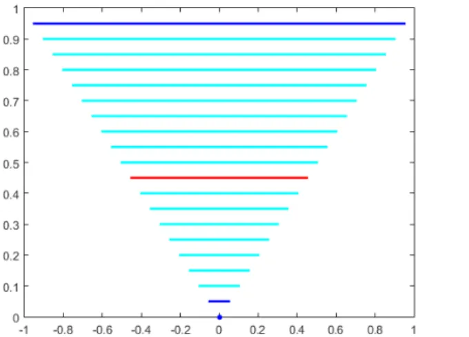
As previously observed, a curve in the plane is a set of points which may be described by an algebraic equation 𝜙 𝒙 0, 𝒙 ∈ 𝑆 or a map 𝒙: 𝐼 → ℝ , where 𝐼 𝑎, 𝑏 ⊂ ℝ. We are interested in the situation where the curve de-pends upon a random variable 𝒀 ∈ ℝ : the equation becomes 𝜙 𝒙|𝒀 𝒚 0 , 𝒙 ∈ 𝑆 𝒚 and the map reads as 𝒙 𝑡|𝒚 : 𝐼 𝒚 → ℝ𝟐. For instance, let us consider the family defined by:
𝜙 𝒙|𝑦 𝑥 𝑦 0, 𝑆 𝑦 𝑥: |𝑥 | 𝑦 1
We have:
𝒙 𝑡|𝑦 𝑡, 𝑦 , 𝑡 ∈ 𝑦, 𝑦 . 2
Assume that 𝑦 ∈ 0,1 is uniformly distributed. The mean value of the parameter is 𝐸 𝑦 1/2 and, for a given 𝑡, the mean value of 𝒙 𝑡|𝑦 is 𝐸 𝒙 𝑡|𝑦 𝑡, 1 |𝑡| /2 Notice that 𝑥 ∈ |𝑡|, 1 . As shown in Figure 1, the means evaluated by this way do not correspond to the family: in fact, they generate a curve similar to the envelope of the family.
As an alternative, we may adopt the standpoint presented in Croquet and Souza de Cursi 2010 : let us intro-duce a fixed interval 𝐽 𝛼, 𝛽 and take 𝑠 ∈ 𝐽 to describe all the curves of the family by using this variable. Here, 𝒙 𝑠|𝑦 2 𝑠 𝛼 𝛽 𝛼 𝑦/ 𝛽 𝛼 , 𝑦 , 𝑠 ∈ 𝛼, 𝛽 . Then, assuming regularity, we determine the expansion of 𝒙 𝑠|𝑦 in a convenient Hilbert basis and the mean of the coefficients:
𝒙 𝑠|𝑦 ∑ 𝒙 𝑦 𝜑 𝑠 ⇒ 𝐸 𝒙 𝑠|𝑦 ∑ 𝐸 𝒙 𝑦 𝜑 𝑠 . 3
In this simple example, we may use a polynomial basis and we obtain:
𝐸 𝒙 𝑠|𝑦 2 𝑠 𝛼 𝛽 𝛼 / 2 𝛽 𝛼 , 1/2 , 𝑠 ∈ 𝛼, 𝛽 4
so that the mean is a member of the family. Nevertheless, the approach introduced by Croquet and Souza de Cursi 2010 requests that the family is composed of parameterized curves. If the parameterization is missing, this method cannot be applied – it is necessary to determine a parameterization previously. In this work, we examine an alternative approach which may be applied without parameterization: we look for one of the elements of the family having a median position, id est, for a member of the family which occupies a central position and may be considered as a good representative of the family. In such a case, we look for the element of the family which is the nearest one for all the others. This is performed by minimizing the distance between nonparameterized curves – we use the Hausdorff distance HD defined in equation 17 . Figure 2 shows the obtained result when this method is applied to the previous example.
Figure 2: The median curve red and the curves defining the “confidence interval” cyan are members of the family Once the median curve is determined, we may look for a “confidence interval” by finding a region including the mean curve and containing a given percentage of the family: usually, confidence intervals use a parameter 𝜶 – the risk – and a confidence level 𝟏 𝜶. For instance, we may look for a “confidence interval” having a level 𝟗𝟎 % thus, 𝜶 𝟏𝟎 % by finding a region containing the 90% members of the family which are closer to the median curve, as shown in Figure 2. More generally, the difficulty exposed concerns the determination of the mean or the median of families of curves. Let us illustrate the situation by considering different families of random curves.
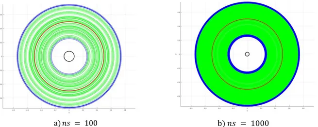
2.1 A family of random circles
Let us consider a family of circles having a random radius and a random initial phase: 𝑥 𝑡 𝑟 ∗ cos 𝑡 𝛼
𝑦 𝑡 𝑟 ∗ sin 𝑡 𝛼 5
Figure 3: The pointwise mean circle in black in near the origin, the median generated by examining the Hausdorff dis-tances in red is central. green circles correspond to the confidence interval
2.2 A family of random arcs of circles
Let us consider a family of random arcs of circles generated as follows: 𝑥 𝑡 𝑎 cos 𝑡 𝛼
𝑦 𝑡 𝑏 sin 𝑡 𝛼 6
where 𝑡 ∈ 0 , 𝜋/4 , 𝛼 is uniformly distributed on 0,2𝜋 , 𝑎 and 𝑏 are uniformly distributed on 1,1 . For independent variables, 𝐸 𝑥 𝑡 𝐸 𝑦 𝑡 0.
As previously done with circles, we consider samples of 𝑛𝑠 100 at left in Figure 4 and 𝑛𝑠 1000 at right in Figure 4 . Green arcs lay in the confidence interval with a risk 𝛼 10%. Blue segments are outside this confi-dence interval – as expected these are the outermost ones. As in the preceding example, the blue curves represent 10% of the sample and the pointwise mean furnishes a small curve near the origin, that goes to zero when the size of the sample increases.
Figure 4: The pointwise mean arc of circle in black reduces to a point, the median one generated by examining the Hausdorff distances in red , and the confidence interval green arcs of circle
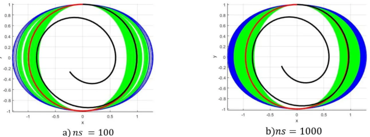
2.3 A Van der Pol oscillator with a random initial position As a third example, we consider a Van der Pol oscillator
𝑥 𝑥 𝑎 𝑥 𝑥 , 𝑥 0 𝑥 ; 𝑥 0 0 . 7
exhibit the statistical characteristics of interest from this family. In this case again, the mean curve is not a trajectory of the system, while the median is a member of the family. The results are displayed in Figure 5 considering the confidence interval at the same level used before. It is interesting to notice that, in this case, the confidence interval may be considered as unilateral.
Figure 5: The results for the Van der Pol oscillator with random initial position: pointwise mean black curve is not a trajectory, while the median red curve is a feasible trajectory. Green curves correspond to the confidence interval.
2.4 A Duffing oscillator with random parameters A last example is given by the Duffing oscillator:
𝑥 𝑎𝑥 𝑏𝑥 , 𝑥 0 𝑥 ; 𝑥 0 1 . 8
We consider 𝑎 is uniformly distributed on 0.5, 1.5 , and 𝑏 uniformly distributed on 0.1, 0.2 . The results are exhibited in Figure 6. We observe that the pointwise mean does not correspond to a trajectory in the phase space, while the median is a feasible trajectory.
Figure 6: Results for the Duffing oscillator with random parameters: pointwise mean black curve is not a trajectory, while the median red curve is a feasible trajectory. Green curves correspond to the confidence interval.
As established in the preceding examples, this approach is effective to furnish the median and, then, to generate a confidence interval of a family of curves, so that we may consider its application to the determination of the mean and a confidence interval of Pareto’s fronts. In the sequel, this method is used in order to quantify uncertainties in MOO problems. Initially section 6 , it is applied to three classical test problems and then section 7 , to the analysis of a 5 bar truss structure MOO problem.
3 DETERMINISTIC MULTIOBJECTIVE OPTIMIZATION
⎩ ⎪ ⎨ ⎪
⎧Minimize𝒙∈ℝ 𝒇 𝒙|𝒚 𝑓 𝒙|𝒚 , 𝑓 𝒙|𝒚 , … , 𝑓 𝒙|𝒚
Subject to
𝒈 𝒙|𝒚 𝑔 𝒙|𝒚 , … , 𝑔 𝒙|𝒚 𝟎 𝒉 𝒙|𝒚 ℎ 𝒙|𝒚 , … , ℎ 𝒙|𝒚 𝟎
𝒙 𝒙 𝒙
, 𝒙 , 𝒙 ∈ ℝ ℝ 9
or more simply: Minimize
𝒙∈ℝ 𝒇 𝒙|𝒚 𝑓 𝒙|𝒚 , 𝑓 𝒙|𝒚 , … , 𝑓 𝒙|𝒚
Subject to 𝑆 ⊂ ℝ𝒙 ∈ 𝑆 10
In these two systems:
• 𝑓1, 𝑓2, … , 𝑓𝑛are the objective functions • 𝑔1, 𝑔2… , 𝑔𝑝 are the inequality constraints • ℎ1, ℎ2… , ℎ𝑘 are the equality constraints
• 𝒙 𝑥 , 𝑥 , … , 𝑥 ∈ ℝ is the decision variables vector • 𝒙𝒍 (resp. 𝒙𝒖) is the lower boundary (resp. upper boundary)
• 𝒚 𝑦 , 𝑦 , … , 𝑦 ∈ ℝ represents the values of the exogenous parameters • 𝑆𝑛 is the feasible space including all the constraints and boundaries above
Numerous methods can be used to solve deterministic MOO problems, such as the weighting method Gass and Saaty 1955 and Zadeh 1963 , the å-constraint method Haimes et al. 1971 , Geoffrion-Dyer-Feinberg Method Geoffrion et al. 1972 , the Keeney-Raiffa method Keeney and Raiffa 1994 and more see for instance: Miettinen 1999 and Collette and Siarry 2002 and in this work we use a variational method called here the Zidani-Souza’s method that has been proposed by Zidani et al. 2013 and which is presented in the appendix A. It consists in minimizing the hypervolume between the Pareto front and the utopia point. In this method, the decision variables are developed in polynomials, what allows to get a piecewise continuous Pareto front.
4 MULTIOBJECTIVE OPTIMIZATION UNDER UNCERTAINTIES
To take the uncertainties into account, we introduce the random vector 𝒀 of exogenous variables, in replace-ment of the deterministic vector 𝒚. As a consequence, both objective functions and constraints become random. In this case, equality and inequality constraints become probabilistic and the standard MOO problem becomes:
⎩ ⎪ ⎨ ⎪
⎧ Minimize𝒙∈ℝ 𝑭 𝒙|𝒀 𝐹 𝒙|𝒀 , 𝐹 𝒙|𝒀 , … , 𝐹 𝒙|𝒀
Subject to Prob 𝑮 𝒙|𝒀Prob 𝑯 𝒙|𝒀 𝐻 𝒙|𝒀 , … , 𝐻 𝒙|𝒀𝐺 𝒙|𝒀 , … , 𝐺 𝒙|𝒀 𝟎𝟎 𝛼𝛽
𝒙 𝒙 𝒙
, 𝒙 , 𝒙 ∈ ℝ ℝ 11
where Prob is the probability operator, 𝒀 has a given joint probability distribution, and 𝛼 and 𝛽 are the reliability probabilities that are imposed by the decision maker. Then, each realization 𝒚 𝑦, , 𝑦, , … , 𝑦 , of 𝒀 leads to a
unique deterministic MOO problem that generates a piecewise continuous Pareto front, and a sample 𝒚 , 𝒚 , … , 𝒚 of 𝒀 leads to 𝑛𝑠 distinct MOO problems and a set of 𝑛𝑠 different curves or hypersurfaces .
As previously mentioned, the main goal of this work is to focus on uncertainties in MOO; more precisely, a link is established between Geometry and Statistics when the randomness of an exogenous variable lead to a set of Pareto fronts instead of one front. In fact, our objective is to evaluate statistical quantities, namely confidence in-tervals of a set from the single data furnished by the set itself, without the use of an external probability – they are generated by using “means” or “medians” . Then, considering randomness on a MOO problem inputs, we explore the outputs, namely the trade-offs, and extract from the family its “median” and other “quantile curves”, more gen-erally the hypersurfaces that belong also to the same set. In other words, we search for a mean of a set of subjects that is one of its members.
5 IMPLEMENTATION
In practice, the approach under consideration is implemented as follows:
• By using a Monte Carlo simulation, we get for each m-tuple 𝒚𝑖 𝑦𝑖,1, 𝑦𝑖,2, … , 𝑦𝑖,𝑚 tsuch as 1 𝑖 𝑛𝑠 a new MOO problem. In this work we focus on the bi-objective optimization problems with inequality constraints, then, theoretically, each value of the sample, leads to a new problem defined as follows:
⎩ ⎨
⎧ Minimize𝒙∈ℝ 𝒇 𝒙|𝒚 𝑓, 𝒙|𝒚 , 𝑓, 𝒙|𝒚 , 𝑖 ∈ 1,2, … , 𝑛𝑠
Subject to Prob 𝑔 𝒙|𝒚 𝑔 𝒙|𝒚 , … , 𝑔 𝒙|𝒚 0 𝛼
𝒙 𝒙 𝒙
, 𝒙 , 𝒙 ∈ ℝ ℝ 12
• Each problem is solved by using the Zidani-Souza’s method and 𝑛𝑠 Pareto fronts denoted 𝑆𝑖∗are obtained.
• We compute the sum of the distances between each Pareto front and all the other ones:
𝐷 ∑ 𝑑 𝑆∗, 𝑆∗ 13
where 𝑑 𝑆∗, 𝑆∗ is a well-chosen distance.
• The mean Pareto front is defined as:
𝑆̅ 𝑆∗ such as 𝑆∗ ∈ 𝑆∗, 𝑆∗, … , 𝑆∗
𝐷 min 𝐷 | 𝑖 ∈ ⟦1, 𝑛𝑠⟧ 14
• The x%-quantile-hypersurfaces:
𝑆 % 𝑆∗ such as Prob 𝐷 𝑑𝑆 ∈ 𝑆 𝑥 15
where 𝐷 is a random variable taking values in the resulting set 𝐷 , 𝐷 , … , 𝐷 . In this work, we consider two distances:
1) The L2 distance given by:
𝑑 𝑆∗, 𝑆∗ 𝐹 𝐹
𝑓, 𝒙|𝒚 𝑓, 𝒙|𝒚 𝑓, 𝒙|𝒚 𝑓, 𝒙|𝒚 ; 𝑖, 𝑗 ∈ ⟦1, 𝑛𝑠⟧ 16
2) The Hausdorff distance given by:
𝑑 𝑆∗, 𝑆∗ max sup ∈ ∗𝛿 𝑥, 𝑆
∗ , sup ∈ ∗𝛿 𝑦, 𝑆
∗ ; 𝑖, 𝑗 ∈ ⟦1, 𝑛𝑠⟧ 17
where 𝑆∗ and 𝑆∗ are closed bounded non-empty subsets of the metric space ℝ , 𝛿 .
In a first step, we considered both the distances: tests running with each one provided results that were com-pared and showed to be almost identical. Then, in a second step, we considered the single Hausdorff distance and a larger sample 𝑛𝑠 200 to determine the quantities of interest.
6 TEST FUNCTIONS
In this section, three academic test functions are considered. All are solved as deterministic problems before uncertainties are considered. All the problems are bi-objective, involving constraints, as previously mentioned. 6.1 Binh and Korn function
The original problem is reported in Binh and Korn 1997 and is as follows:
Minimize𝒙∈ℝ 𝑓 𝒙𝑓 𝒙 𝑓 𝑥 , 𝑥𝑓 𝑥 , 𝑥 𝑥4𝑥5 4𝑥 𝑥 5
Such that 𝑥𝑥 85 𝑥𝑥 325 7.7 0 𝑥 5 , 0 𝑥 3
By applying Zidani-Souza’s method of the appendix A, this problem is efficiently solved by expanding 𝑥 and 𝑥 as polynomials of degree 6, having their coefficients in 𝑐 , 𝑐 10,10 . The numerical results are as following:
𝒙∗ argmin
𝒙 ∈ 𝑓 𝒙 0,0
𝒙∗ argmin
𝒙 ∈ 𝑓 𝒙 5,3
𝒇 𝑓 𝒙∗ , 𝑓 𝒙∗ 0,4
𝐴 rot 𝒑∗ 𝑡 ∇𝒑∗ 𝑡 d𝑡 ∈ ,
1431
⟨ . | . ⟩ being the scalar product, rot 𝒑∗ . the rotational of 𝒑∗and 𝐴 is the area or hypervolume that was
minimized and that is bounded by the utopia point and the Pareto front given by 𝒑∗ 𝑓∗, 𝑓∗ .
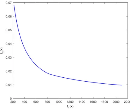
The corresponding Pareto front is presented in Figure 7.
Figure 7: Pareto front of the Binh and Korn test function
To make the problem uncertain, we introduce randomness in the 2nd objective function by using two
uncorre-lated random variables 𝜉 and 𝜉 that are uniformly distributed on 0,1 :
Minimize𝒙∈ℝ 𝑓 𝒙 𝑓 𝒙𝑥 4 𝑥0.2𝜉 𝜉5 4 𝑥𝑥 0.2𝜉𝜉 5
Such that 𝑥𝑥 85 𝑥𝑥 325 7.7 0 𝑥 5 , 0 𝑥 3
Figure 8: Binh and Korn function under uncertainties for ns 200 sample size: the median Pareto front appears in red, the confidence interval in green and the Pareto fronts beyond the 90%-quantile in blue
Since there are no uncertainties in constraints, they must be satisfied at a 100% level of probability for the problem solution. Figure 8 shows the 200 Pareto fronts obtained, with the mean front in red, the 180 nearest fronts to the mean in green and the 20 farthest ones - in the sense of Hausdorff’s distance - in blue. Thus, the green curves correspond to the 90% closer to the median in the sense of Hausdorff’s distance and may be considered as belong-ing to a confidence interval with risk į 10%. We observe that, as expected, the median is a central curve and the curves laying outside the confidence interval are the outermost ones.
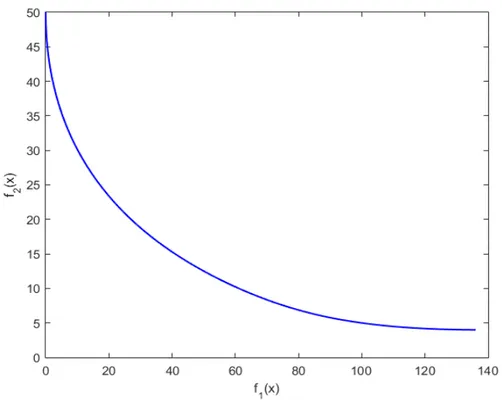
6.2 Fonseca and Fleming function
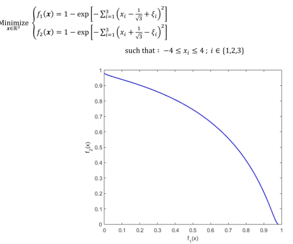
The Fonseca and Fleming problem Fonseca and Fleming 1995 is:
Minimize𝒙∈ℝ 𝑓 𝒙 1 exp ∑ 𝑥 √
𝑓 𝒙 1 exp ∑ 𝑥 √ 20
such that ∶ 4 𝑥 4 ; 𝑖 ∈ 1,2,3
Here yet, polynomials of the 6th. degree with coefficients on c , c 10,10 are considered. The
nu-merical results are the following, and the Pareto front is shown in Figure 9:
𝒙∗ argmin 𝒙 ∈ 𝑓 𝒙
1 √3,
1 √3,
1 √3
𝒙∗ argmin 𝒙 ∈ 𝑓 𝒙
1 √3,
1 √3,
1 √3 𝒇 𝑓 𝒙∗ , 𝑓 𝒙∗ 0,0
𝐴 ⟨rot 𝒑∗ 𝑡 |∇𝒑∗ 𝑡 ⟩d𝑡 ∈ ,
Three uncorrelated random variables 𝜉 , 𝜉 and 𝜉 that are all uniformly distributed on 0,0.1 are added to this system in order to make it uncertain, then 𝑛𝑠 200 deterministic problems derived from the initial one are obtained as follows:
Minimize
𝒙∈ℝ
𝑓 𝒙 1 exp ∑ 𝑥 √ 𝜉
𝑓 𝒙 1 exp ∑ 𝑥 √ 𝜉 21
such that ∶ 4 𝑥 4 ; 𝑖 ∈ 1,2,3
Figure 9: Pareto front of the Fonseca and Fleming test function
Figure 10 shows the 200 curves we get and the mean that minimizes both of the distances that we used is in the middle of the curves set as expected.
In this case 𝑓 𝑓 𝒙 is a concave function, furthermore, all of the Pareto fronts ends are located together is a small region of space. In this case, the Hausdorff distance exhibits a larger variation in the middle of the family of curves, so that the curves beyond the 90%-quantile in blue appear more clearly when compared to the preceding situation. Notice that the median appears as a mean curve, in the center of the family.
6.3 Zitzler-Deb-Thiele's function 3 ZDT3
Let us consider the function 𝑔 of 𝒙 𝑥 , 𝑥 , … , 𝑥 defined such as:
𝑔 𝒙 1 ∑ 𝑥 22
Then, the ZDT3 Problem, which is reported in Zitzler et al. 2000 reads as follows:
Minimize𝒙∈ℝ ⎩ ⎨
⎧ 𝑓 𝒙 𝑥
𝑓 𝒙 1 𝒙𝒙 𝒙𝒙 sin 10𝜋𝑓 𝒙 0 𝑥 1 𝑖 ∈ 1,2, … , 𝑛
23
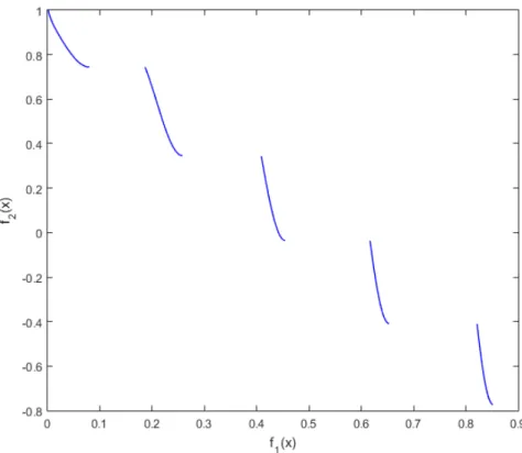
Here we consider the case 𝑛 2. The Pareto front of this problem is given in Figure 11.
Figure 11: Pareto front of the ZDT3 test function
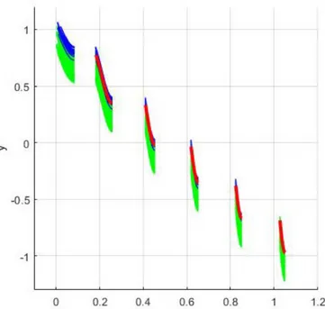
In order to make the problem uncertain, we introduce two uncorrelated random variables 𝜉 and 𝜉 that are uniformly distributed on 0,1 and on 0.15,0.15 , respectively. Then, we consider
𝑓 𝒙 𝑥 𝜉
𝑓 𝒙 1 𝜉 𝒙𝒙 𝒙𝒙 sin 10𝜋𝑓 𝒙 24
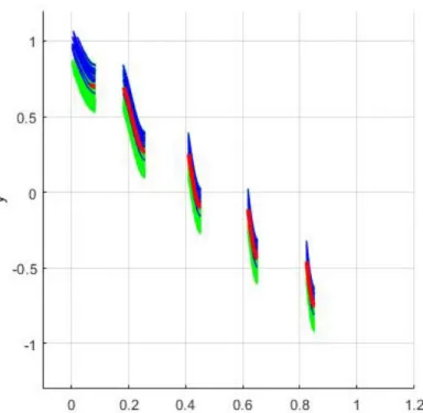
Figure 12: Pareto fronts of the ZDT3 test function involving uncertainties: for 𝑛𝑠 200: the median Pareto front appears in red, the confidence interval in green and the Pareto fronts beyond the 90%-quantile in blue
In this case, the Pareto’s front is discontinuous. This fact makes that Hausdorff’s distances between curves that seem close to the eye are, in fact, large in the sense of Hausdorff’s distance. This fact is due to the fact that some parts of a curve may be isolated from the other curve, so that the distance of these points to the other one is large. For instance, let us consider the fronts shown in Fig. 13: the blue front may appear to the eye as being closer to the red one than the green front, but the respective Hausdorff’s distances are 0.4132 and 0.1975, so that the green front is closer to the red one in the Hausdorff’s sense. Observe that the red front has points which are far from the blue one.
Figure 13: The blue front may appear as closer to the median in red than the green one, but its Hausdorff’s distance is the greatest one.
Figure 14: ZDT3 median Pareto front red and confidence interval green when the last arc is ignored.
7 APPLICATION ON A 5-BAR TRUSS STRUCTURE
In this section we study the five-bar truss structure sketched in Figure 15, where we minimize its total mass denoted 𝑤, simultaneously with its maximum displacement denoted 𝑢 Ellaia et al. 2013 . Then we introduce un-certainties on some parameters to see how the solution set behaves when the system values change.
It is assumed that the structure will be modeled by linear, two nodes, bar elements in linear elasticity, subjected only to axial forces and free from imperfections. The geometric and material parameters used are length 𝑙 9.3144 m, area 𝑎 0.01419352 m , load 𝑝 448.2 kN, Young′s modulus
𝑒 68.95 GPa, density 𝜌 2,768 kg m⁄ and yield stress 𝜎 172.4 MPa.
Figure 15: 5 bar truss structure schema
Denoting 𝒙 ∈ ℝ the vector of the topological and sizing optimization parameters, such that 0 𝑥 1 for 𝑖 ∈ 1, 2, … , 𝑛 where 𝑛 5 is the number of elements, the problem to solve is:
Minimize𝒙∈ℝ 𝑓 𝒙 𝑢 max 𝒖 𝑓 𝒙 𝑤 ∑∗ argmin 𝒖 𝒌 𝒙 𝒖 𝒖 𝒇𝜌 𝑎𝑙 𝑥 25
Such that ∶ 𝜎 𝜎 , 1 𝑖 𝑛
With a 6 degree polynomial 𝝋 and 𝑐 10, we get the Pareto front in Figure 16.
Figure 16: Pareto front of the 5 bar truss structure
In the next step we consider:
• the force 𝑝 that becomes uncertain (denoted 𝑃) following a normal distribution with 10% for the coefficient of variation.
• the Young modulus 𝑒 that becomes uncertain too (denoted 𝐸) following a truncated normal distribution defined on 60.68 , 77.22 GPa with 3% for the coefficient of variation.
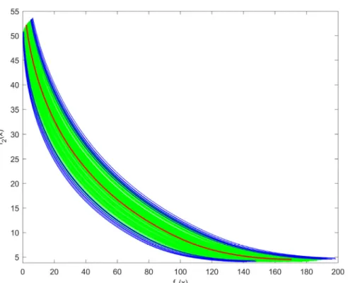
As done with the test functions, ns 200 problems are generated with a MCS and the result we obtained is shown in Figure 17:
In Figure 17, results are “as expected”: the mean is in the middle of the curves set, while curves beyond the 90%-quantile in blue are located at the exterior of the curves set.
8 Summary
In this work, the MOO problems with constraints and uncertainties are addressed. Instead of analyzing a cloud of data points, the adopted point of view consists of analyzing the randomness of objects that can be modeled by continuous geometric forms, thanks to the Zidani and Souza de Cursi's method which leads to a piecewise continu-ous Pareto front for the MOO problems, and curves distances measures. Hence, by using a Monte Carlo simulation, a sample of Pareto fronts is generated and the Hausdorff’s distance leads to a Pareto front quantile analysis, from the link that we made between Statistics and Geometry. Three academic problems are first modified to handle un-certainties and then solved. Next, an application to a 5-bar truss structure with two exogenous random variables is considered to demonstrate the applicability of the proposed method with a more difficult problem. All results ob-tained appear satisfactory when observing the location of the median curve and quantiles.
A possible perspective of this work is to apply the approach presented in this paper to a MOO problem under uncertainties where objective functions and constraints are expended with Generalized Fourier Series Bassi et al. 2016 . The use of approximated functions instead of the initial ones aims to reduce the algorithms running time.
Example 6.3 shows that Hausdorff’s distance may lead to results that may be considered as unexpected from the eye’s point of view. We may find in the literature modifications of Hausdorff’s distance see, for instance, Dubu-isson and Jain, 1994 - different distances may be used with the procedure exposed in this work. The comparison between the existing distances and the definition of criteria for the selection of the adequate one will be matter of further work.
References
Amodeo L., Chen H., El Hadji A. 2007 , Multi-objective Supply Chain Optimization: An Industrial Case Study. In: Giacobini M. eds Applications of Evolutionary Computing. EvoWorkshops 2007. Lecture Notes in Computer Sci-ence, vol 4448. Springer, Berlin, Heidelberg
Bachur, W.E. G., Gonçalves, E. N., Ramírez, J. A., Batista, L. S. 2017 A multiobjective robust controller synthesis approach aided by multicriteria decision analysis, Applied Soft Computing, Volume 60, pages 374-386, https://doi.org/10.1016/j.asoc.2017.06.027.
Bassi, M., Souza de Cursi, J. E., Ellaia, R. 2016 Generalized Fourier Series for Representing Random Variables and Application for Quantifying Uncertainties in Optimization, 3rd International Symposium on Uncertainty Quantifi-cation and Stochastic Modeling, Maresias, SP, Brazil, February 15-19, 2016
Bawa, V. S. 1975 Optimal rules for ordering uncertain prospects, Journal of Financial Economics, Volume 2, Issue 1, pages 95-121, https://doi.org/10.1016/0304-405X 75 90025-2.
Bawa, V. S. and Goroff, D. L 1983 Stochastic dominance, efficiency and separation in financial markets, Journal of Economic Theory, Volume 30, Issue 2, pages 410-414, https://doi.org/10.1016/0022-0531 83 90115-1.
Binh, T. and Korn, U. 1997 MOBES: A Multiobjective Evolution Strategy for Constrained Optimization Problems. In: Proceedings of the Third International Conference on Genetic Algorithms. Czech Republic, 176-182
Collette, Y. and Siarry, P. 2002 Optimisation multiobjectif, Eyrolles, Paris
Craven, B. D. and Islam, S. M. N. 2005 , Optimization in Economics and Finance: Some Advances in Non-Linear, Dynamic, Multi-Criteria and Stochastic Models, Springer, USA
Dubuisson, M.-P and Jain, A.K. 1994 . A modified Hausdorff distance for object matching. Proceedings of the 12th IAPR International Conference. Vol. 1. 566 - 568 vol.1. 10.1109/ICPR.1994.576361.
Ellaia, R., Habbal, A. and Pagnacco, E. 2013 A New Accelerated Multi-objective Particle Swarm Algorithm: Appli-cations to Truss Topology Optimization, 10th World Congress on Structural and Multidisciplinary Optimization, Orlando, Florida, USA
Fonseca, C. M. and Fleming, P. J. 1995 , An overview of evolutionary algorithms in multiobjective optimization, Evolutionary Computation, 3:1: 1-16.
Gass, S. and Saaty, T. 1955 , The computational algorithm for the parametric objective function. Naval Research Logistics, 2: 39-45. doi:10.1002/nav.3800020106
Geoffrion, A.M., Dyer, J.S., and Feinberg, A. 1972 , An Interactive Approach for Multi-Criterion Optimization, with an Application to the Operation of an Academic Department, Management Science 19, No.4, 357-368.
Hadar, J., Russell, W. 1969 . Rules for Ordering Uncertain Prospects. American Economic Review. 59 1 : 25–34.
Haimes, Y.Y., Lasdon, L.S. and Wismer, D.A. 1971 On a Bicriterion Formulation of the Problems of Integrated Sys-tem Identification and SysSys-tem Optimization, IEEE Transactions on SysSys-tems, Man, and Cybernetics 1, 296-297. doi:10.1109/tsmc.1971.4308298
Hurson, Ch and Zopounidis, C. 1997 , On The Use Of Multicriteria Decision Aid Methods To Portfolio Selection, Springer, Berlin, Germany
Ivanov, S. Y. and Ray, A. K. 2014 , Multiobjective Optimization of Industrial Petroleum Processing Units Using Ge-netic Algorithms, Procedia Chemistry, 10:2014: 7-14. doi: 10.1016/j.proche.2014.10.003
Ji, R. and Lejeune, M.A. 2018 Risk-budgeting multi-portfolio optimization with portfolio and marginal risk con-straints Ann Oper Res 262: 547. https://doi-org.ezproxy.normandie-univ.fr/10.1007/s10479-015-2044-9
Keeney, R.L. and Raiffa, H. 1994 Decisions with multiple objectives–preferences and value tradeoffs, Cambridge University Press, Cambridge & New York, 1993, 569 pages, ISBN 0-521-44185-4 hardback , 0-521-43883-7 pa-perback . Syst. Res., 39: 169-170. doi:10.1002/bs.3830390206
Light, B. 2018 Precautionary saving in a Markovian earnings environment, Review of Economic Dynamics, Vol-ume 29, pages 138-147, https://doi.org/10.1016/j.red.2017.12.004.
Mankiw, N.G. 2011 , Principles of Economics - 6th edition, Southwestern College Publishing, Tennessee, USA
Miettinen, K. 1999 Nonlinear multiobjective optimization, Kluwer Academic Publishers, Boston, 1999
Moreira, F. R., Lobato, F. S., Cavalini Jr, A. A., Steffen Jr, V. 2016 . Robust Multi-objective Optimization Applied to Engineering Systems Design. Latin American Journal of Solids and Structures, 13 9 , 1802-1822. https://dx.doi.org/10.1590/1679-78252801
Navabi, M. and Mirzaei, H. 2017 Robust Optimal Adaptive Trajectory Tracking Control of Quadrotor Helicopter. Latin American Journal of Solids and Structures, vol.14, no.6, p.1040-1063. http://dx.doi.org/10.1590/1679-78253595
Sahinidis, N. V. 2004 , Optimization under uncertainty: state-of-the-art and opportunities, Computers and Chemi-cal Engineering, 28: 971–983. doi: 10.1016/j.compchemeng.2003.09.017
Souza de Cursi, E. 2015 , Variational Methods for Engineers with Matlab, Wiley
Varian, H. 2006 , Microeconomic Analysis, Cram101 Inc., USA
Varian, H. 2009 , Intermediate Microeconomics: A Modern Approach, - 8th edition, W. W. Norton & Company
Xidonas, P., Mavrotas, G., Hassapis, C., Zopounidis, C. 2017 Robust multiobjective portfolio optimization: A mini-max regret approach, European Journal of Operational Research, Volume 262, Issue 1, pages 299-305, https://doi.org/10.1016/j.ejor.2017.03.041.
Yager, R. R. 2018 Refined expected value decision rules, Information Fusion, Volume 42, pages 174-178, https://doi.org/10.1016/j.inffus.2017.10.008.
Zadeh, L. 1963 , Optimality and Non-Scalar Valued Performance Criteria, IEEE Transactions on Automatic Control 8, 59-60. doi:10.1109/tac.1963.1105511
Zidani, H., Ellaia, R., and Souza De Cursi, E. 2013 Representation of solution for multiobjective optimization: RSMO for generating a Su sant Pareto front, Proceedings of 2013 International Conference on Industrial Engineering and Systems Management IESM , Rabat, 2013, pp. 463-463.
Zitzler, E., Deb, K. and Thiele, L. 2000 Comparison of multi-objective evolutionary algorithms: Empirical results. Evolutionary Computation, 8 2 , 173-195, 2000.
Zopounidis, C. 1999 , Multicriteria Decision Aid in Financial Management, European Journal of Operational Re-search, 119:2: 404-415. doi: 10.1016/S0377-2217 99 00142-3.
Appendix A
THE VARIATIONAL APPROACH FOR THE MULTI-OBJECTIVE OPTIMIZATION PROBLEM
In this appendix, we explain the variational approach that leads to the Zidani-Souza’s method used in this work, originally proposed in Zidani et al. 2013 and in Souza de Cursi 2015 .
Let us consider two objective functions 𝑓 and 𝑓 having as individual minima: 𝒙𝟏∗ argmin
𝒙∈ 𝑓 𝒙
𝒙𝟐∗ argmin 𝒙∈ 𝑓 𝒙
26
We look for a curve connecting these two points, defined by an unknown vector of parameters 𝒄:
𝒙 𝒄, 𝑡 𝑥 𝒄, 𝑡 , 𝑥 𝒄, 𝑡 , … , 𝑥 𝒄, 𝑡 𝒙𝟐∗ 𝒙𝟏∗ . 𝑡 𝒙𝟏∗ 𝝋 𝒄, 𝑡 27
The variable 𝑡 is assumed to belong to 0,1 . Since 𝒙𝟏∗ and 𝒙𝟐∗ belong to the curve, we have:
∀𝒄 ∶ 𝝋 𝒄, 0 𝝋 𝒄, 1 𝟎 28
A simple choice consists in using polynomials, such as, for instance
𝝋 𝑡 ∑ 𝒄.𝒊 𝑡 1 𝒄.𝒏 𝑡 1 with 𝒄.𝒏 ∑ 𝒄.𝒊 , 𝒄.𝒊∈ ℝ 29
where 𝒄.𝒊 stands for the ith column of the coefficient matrix 𝒄.
Taking the last condition into account, we may look for
𝝋 𝑡 ∑ 𝒄.𝒊 𝑡 𝑡 , 𝒄.𝒊∈ ℝ 30
In order to solve a given MOO problem, let 𝒄.𝟏, 𝒄.𝟐, … , 𝒄.𝒏 be varying into a set C that we choose in compliance
with the situation under consideration. The Pareto front is obtained by minimizing the hypervolume between the curve 𝒑 𝑐, 𝑡 𝑓 𝒙 𝒄, 𝑡 , 𝑓 𝒙 𝒄, 𝑡 , 𝑡 ∈ 0,1 and the utopia point, or by maximizing the hypervolume be-tween this curve and the anti-utopia point Figure 18 . In this work, we apply the first method by using the Stokes formula that allows the use of the integration on a curve instead of the integration on a surface:
𝐴 𝒄 ∈ , rot 𝒑 𝒄, 𝑡 𝛻𝒑 𝒄, 𝑡 𝑑𝑡 31
where rot 𝒑 stands for the rotational of 𝒑. Once we solve the problem:
𝒄𝒔𝒐𝒍 argmin 𝐴 𝒄 32
we get the Pareto front 𝑆 of ℝ as: 𝑆 𝒑∗ 𝑐, 𝑡 𝑓 𝒙 𝒄
𝒔𝒐𝒍, 𝑡 , 𝑓 𝒙 𝒄𝒔𝒐𝒍, 𝑡 , 𝑡 ∈ 0,1 33