MULTIOBJECTIVE ENGINEERING DESIGN OPTIMIZATION PROBLEMS: A SENSITIVITY ANALYSIS APPROACH
Oscar Brito Augusto
1*, Fouad Bennis
2and Stephane Caro
3Received August 5, 2011 / Accepted July 20, 2012
ABSTRACT.This paper proposes two new approaches for the sensitivity analysis of multiobjective design optimization problems whose performance functions are highly susceptible to small variations in the design variables and/or design environment parameters. In both methods, the less sensitive design alternatives are preferred over others during the multiobjective optimization process. While taking the first approach, the designer chooses the design variable and/or parameter that causes uncertainties. The designer then associates a robustness index with each design alternative and adds each index as an objective function in the optimization problem. For the second approach, the designer must know, a priori, the interval of variation in the design variables or in the design environment parameters, because the designer will be accepting the interval of variation in the objective functions. The second method does not require any law of probability distribution of uncontrollable variations. Finally, the authors give two illustrative examples to highlight the contributions of the paper.
Keywords: multiobjective optimization, Pareto-optimal solutions, sensitivity analysis.
1 INTRODUCTION
Many engineering design problems are multiobjective by nature, because they often involve more than one design objective to be optimized. These design objectives impose potentially conflicting requirements on the technical and economic performance of a given system. A designer must formulate an optimization problem with multiple objectives if he/she wishes to study the trade-offs that exist between these conflicting objectives and to explore their design options.
Multiobjective engineering design problems often have design parameters with uncontrollable variations due to noise or uncertainties. Such variations can affect outcomes significantly, such as the performances of objective functions and/or the feasibility of the Pareto optimal solutions.
*Corresponding author
1Escola Polit´ecnica da Universidade de S˜ao Paulo – E-mails: [email protected] / [email protected] 2 ´Ecole Centrale de Nantes, Institut de Recherche en Communications et Cybern´etique de Nantes
– E-mail: [email protected]
A robust optimal solution is as good as possible with regard to the objective functions, and it offers the lowest possible sensitivity to variations in design variables and design parameters. In practice, all engineering designs are sensitive to uncertainties that can arise from manufactur-ing operations, variations in material properties, the operatmanufactur-ing environment and other reasons. Moreover, non-robust designs can be expensive to produce or to operate and can fail frequently in service.
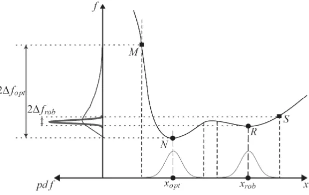
Figure 1 illustrates the solution of a single-objective robust optimization problem. The perfor-mance function f(x)is minimum when the design variable x is equal to xopt. However, the
sensitivity of f(x)to variations inxopt is significant. Indeed,1fopt, which depicts the range
of variations in f(x)for a given range of variations inx aroundxopt, is large. On the contrary, xr obis a local minimum of function f(x), and the sensitivity of f(x)to variations inxr obis very
small. Indeed,1fr ob, which depicts the range of variations in f(x) for a given range of
varia-tions inx aroundxr ob, is small. In fact,1fr ob < 1fopt. Accordingly, xr ob is a good solution
to the single-objective robust optimization problem. In the case of a multiobjective optimization problem, a robust optimum solution may be located in the neighborhood of the Pareto front. Such a solution should have as little sensitivity as possible to uncertainties, because it cannot violate any constraint and/or acceptable known variations in design objectives in the presence of uncer-tainties. In this context, the purpose of this paper is to define a methodology to help the designer choose one or several robust optimum solution(s) when he/she must address a multiobjective robust design optimization problem.
Figure 1– A robust solutionvs.an optimal solution.
Then, two illustrative examples highlight the paper’s contributions. Finally, the conclusions are discussed.
Nomenclature
fi(X) ith objective function
f(X) vector of objective functions
gj(X) jth inequality constraint function K K T Karush-Khun-Tucker
Js global sensitivity Jacobian matrix
Jx sensitivity Jacobian matrix related to the design variables
Jp sensitivity Jacobian matrix related to the design parameters k number of objective functions
m number of inequality constraint functions n number of decision variables
q number of design parameters pi ith design parameter
p vector of design parameters
pi n f,psup lower and upper bounds of the design parameters
R(v) robustness index associated with the design variablesXand the parametersp S feasible region in the decision space
S sensitivity of the objective function
S diagonal matrix with the singular values in the singular value decomposition
U unitary matrix, expressed in the function space, in the singular value decomposition
v vector joining the design variablesXand the parametersp
V unitary matrix expressed in the decision space in the singular value decomposition
xi ith decision variable
xi average of the ith decision variable included in the optimal set
X decision or design variables vector
X∗ non-dominated solution of a multiobjective optimization problem
Xi n f,Xsup lower and upper bounds in the decision space
λj weighting factor for the jth inequality constraint gradient in theK K T condition
1xio interval of a known uniformly distributed variation of theith design variable
1pio interval of a known uniformly distributed variation of theith design parameter
1fio acceptable variation in theith objective function due to1vuncertainties λ vector ofλj s
σi standard deviation for theith decision variable included in the optimal set
ωi weighting factor for theith objective function gradient in theK K Tcondition ω vector ofωi s
2 Definitions of problems
In this section, the formulations of (i) a multiobjective optimization problem, (ii) a robust design problem and (iii) a multiobjective robust optimization problem are given.
2.1 Multiobjective optimization problem
A general multiobjective optimization problem attempts to find the design variablesXthat opti-mize a vector objective functionf(X)over the feasible design spaceS. The determination of a
set of non-dominated solutions, the Pareto optimum solutions or non-inferior solutionsX∗ can achieve a compromise among several objective functions. The problem formulation is defined as follows:
minimize: f(X) (1a)
subject to: gi(X)≤0, i=1,2, . . .m. (1b)
Xinf≤X≤Xsup (1c)
where f(X) =f1,f2,f3, . . . , fkT : Rn → Rk, with fi(X) : Rn → Ras a vector with the
values of objective functions to be minimized.Xis the vector that contains the design variables, also called decision variables, defined in the spaceRn. XinfandXsupare respectively the lower
and upper bounds of the design variables. gi(X) : Rn → Rrepresents theithinequality
con-straint function. Equations (1b) and (1c) define the region of feasible solutions,S, in the decision
variable space. The constraints gi(X)are “less than or equal” functions in view of the fact that
“greater or equal” functions may be converted to the first type if they are multiplied by minus 1. Similarly, the problem deals with the “minimization” of functions fi(X), given that function
“maximization” can be transformed into the former by multiplying it by minus 1.
2.1.1 Pareto optimal solution
The notion of optimum in the context of solving multiobjective optimization problems is known as “Pareto optimal”. A solution is said to be Pareto optimal if there is no alternative to improving one objective without worsening at least one other, that is, the feasible pointX∗Sis Pareto optimal
when there is no other feasible pointX∈Sso∀i,j,fi(X)≤ fi(X∗)with strict inequality in at
least one condition, fj(X) < fj(X∗).
Due to the conflicting nature of the objective functions, the Pareto optimal solutions are usually scattered in the regionS, a consequence of the solutions being unable to minimize the objective
functions simultaneously. Solving the optimization problem achieves a set of Pareto optimal solutions defined in the decision space, after which an image of the objective functions, along with the Pareto front, is calculated over the set of optimal solutions.
2.1.2 Necessary conditions for Pareto optimality
Optimizing the multiobjective problems that are expressed by Eqs. (1a-1c) are of general char-acter, because the equations represent the problem of single-objective optimization whenk=1. According to Miettinen (1998), as in single-objective optimization problems, the solutionX∗∈S
for the Pareto optimality must satisfy the Karush-Kuhn-Tucker condition, expressed as:
k
X
i=1
ωi∇fi(X∗)+ m
X
j=1
λj∇gj(X∗)=0 (2a)
λjgj(X∗)=0 (2b)
λj ≥0 (2c)
ωi ≥0; k
X
i=1
ωi =1 (2d)
whereωiis the weighting factor, positive, for the gradient of theith objective function, calculated
at pointX∗,∇fi(X∗). λj represents the weighting factor for the gradient of the jth inequality
constraint function∇gj(X∗). It is zero when the associated constraint function is not active,i.e., gj(X∗) <0.
It should be emphasized that the set of Eqs. (2a) to (2d) form the necessary conditions forX∗to be Pareto optimal.
2.2 Robust design problem
The concept of robust design was first used by Taguchi (1993). He introduced the concept of parameter design to improve the quality of a product whose manufacturing process involves significant variability or noise. Robust design aims at minimizing the sensitivity of performance to variations without controlling the causes of these variations. In the last decades, several authors contributed to the formulation and the improvement of robust design problems.
To deal with robustness, a set of design parametersp=p1,p2,p3, . . .pqT should be
consid-ered. Those parameters cannot be adjusted by the designer and are thus uncontrollable, such as the cost of the steel used in ship construction. The design variables
X=
x1,x2,x3, . . .xn T
can also be subjected to uncontrollable variations for the reasons of manufacturing errors, wear-ing or other uncertainties, although their nominal value is fixed.
consider variations in the design variables and parameters. CallingvT =
XTpT
, the problem formulation can be defined as follows:
minimize: f(X,p), (3a)
1f(X,p)
over X=
x1,x2,x3, . . .xn T
(3b)
subject to: gi(X,p)+1gi(X,p)≤0, i=1,2, . . .m. (3c)
Xinf≤X≤Xsup (3d)
v−1vinf≤v≤v+1vsup (3e)
All sets of equation (3) are general for search robust solutions of multiobjective optimization problems.
Sundaresanet al. (1993) developed a procedure that incorporates uncertainties in design vari-ables and variations in constraints due to these uncertainties. Chaseet al. (1996) presented the direct linearization method for tolerance analyses of 2D and 3D mechanical assemblies. Chen
et al. (1996) studied two broad categories of problems, namely, (i)Type 1 problems, which minimize variations in performance caused by variations in noise factors (uncontrollable param-eters), and(ii)Type 2, which minimize variations in performance caused by variations in control factors (design variables). Ben-Tal and Nemirovski (1998, 2002) proposed a study of convex optimization problems for which the data, in the present notation p, is not specified exactly. Instead, the data are known only to belong to a given uncertainty set. They developed models for uncertain Linear, Conic Quadratic and Semidefinite programming problems. Kalsiet al.(2001) introduced a technique to reduce the effects of uncertainty and incorporated flexibility in the design of complex engineering systems involving multiple decision makers. Parkinson (2000) used a deterministic method of robust design to determine the optimum nominal dimensions of an assembly in order to improve the assembly quality. Bertsimaset al. (2004) have proposed a robust constrained optimization method for linear programming problems where the matrix of coefficients belongs to a known uncertainty set that is bounded. They have shown that this kind of problem is still linear programming. Bertsimas and Sim (2004) also focused on linear pro-gramming problems, seeking to reduce the level of conservatism of the robust solutions in terms of probabilistic bounds of constraint violations. They have shown that their method retains the advantages of the linear framework and offers full control over the degree of conservatism for every constraint. Thus, their method provides a probabilistic guarantee that the robust solution will be feasible with high probability.
In the next section, the authors propose a simplified approach to searching for less sensitive alternatives when solving multiobjective optimization problems.
3 A SIMPLIFIED MULTIOBJECTIVE ROBUST OPTIMIZATION PROBLEM
Given that a robust optimal solution is as good as possible with regard to the objective functions and that it is as least sensitive as possible to variations in design variables and design parameters, this section presents two methods where robust design alternatives are preferred over others during the multiobjective optimization process.
First, the designer chooses only the design variables and/or design parameters that are subject to variations. With this information, aRobustness Indexis associated with each design alternative. This index is added as one more function to be optimized. In the second approach, the designer accepts variations in the performance functions, limited in fixed intervals, knowinga priorithe range of variations in the design variables and in the design parameters.
Assuming thatfis of classC2inv, one can expand Eq. (3a) in the neighborhood of the pointv0 and keep only the linear terms. Then, the following equation can be obtained:
δf=Jsδv+e(kδvk2) (4a)
δvT =δXTδpT (4b)
Jx =∂f/∂X (4c)
Jp=∂f/∂p (4d)
Js =JxJp (4e)
where k ∙ k2denotes the Euclidian norm operator and e(v)an error function. Js is the global
sensitivity Jacobian matrix, and it describes the effect of the variations in design variables and design parameters to the performance functions. δXand δp are the variations in the design variables and in the design parameters, respectively.Jx is the(k×n)sensitivity Jacobian matrix
off(v)with respect toX, andJpis the(k×q)sensitivity Jacobian matrix off(v)with respect
top, respectively. If variations in the design variables are not considered, then Js = Jp. If
variations in design parameters are not considered, thenJs =Jx.
Ignoring the error in Eq. (4a), an approach to a robust solution is defined as one that is as least sensitive as possible to any variations in the decision variables and design parameters in its neigh-borhood. Considering1vas a closed normalized unit hyper-sphere centered at pointv in the Euclidean space Rn+q,i.e., k1vk2 = 1, thenJs is a linear application that maps the hyper-sphere in a hyper-ellipsoid in the normalized function space, centered inf(v)and described by the variations1f(v)∈Rk. In Figure 2, three design alternatives are checked for their sensitivity
in the decision variable space. Since the local perturbation in the neighborhood of pointAcauses a large modification in the objective values, this alternative may not be as robust as the alternative
Suppose that pointCin Figure 2 belongs to the Pareto set and that its image is on the Pareto front. If any constraint function is not active at this point, then the hyper-ellipsoid collapses one of its axes. Being a Pareto solution, pointCsatisfies Eq. (2a), and the objective function gradients are linearly dependent. Consequently, the variations in the performance functions occur only along the tangent to the Pareto front.
Figure 2– The sensitivity Jacobian matrix transforms a unitary radius ball in the decision space into an ellipsoid in the function space.
3.1 Robustness index
The geometrical interpretation of Eq. (4a) can help one to define aRobustness Indexin order to qualify a design alternative with regard to its robustness. The sensitivity Jacobian matrix can be decomposed by means of the singular value decomposition as follows:
Js =USVT (5)
whereUis ak-by-korthogonal matrix,Sis ak-by-(k+q)diagonal matrix with non-negative real numbers andVTdenotes the transposition ofV, which is a(n+q)-by-(k+q)orthogonal matrix. The diagonal entries of Sare known as the singular values of Js. The singular value decomposition is a generalization of the decomposition of the eigenvalues and eigenvectors, and this decomposition is applied to a square matrix. Ifλiis an eigenvalue ofJsJTs, then the singular valueσi =√λi. As a geometrical interpretation, the non-zero singular values,σi, are the lengths
of the semi-axes of the hyper-ellipsoid represented in Figure 2, and the related vectors inUare the directions of these semi axes in theRkspace.
LetSbe the sensitivity of the objective functions to variationsδv. Scan be defined as the ratio of the Euclidean norm of variations in the objective functions, namelykδfk2, and the Euclidean
singular valueσminand the largest singular valueσmaxof its global sensitivity Jacobian matrix, Js, namely,
σmin≤S = k
δfk2
kδvk2 ≤
σmax (6)
Equation (6) shows that the lowerσmax is, the lower the upper bound of S will be.
Accord-ingly, the Euclidean norm ofJs, that is, its maximum singular value, can be used as a relevant
Robustness Index:
R(v)=σmax (7)
R(v)makes sense if and only if the terms ofJsare normalized, that is, if they have the same unit. Indeed, the singular values ofJscannot be compared if their units are different.
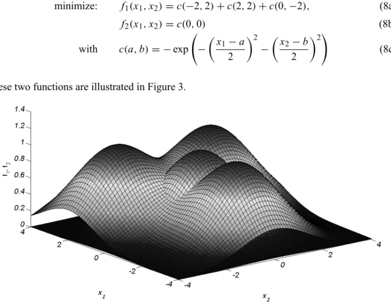
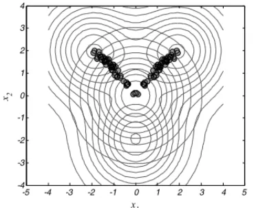
To illustrate the use of such a proposition, let us consider the following unconstrained minimiza-tion problem with two funcminimiza-tions defined inR2space:
minimize: f1(x1,x2)=c(−2,2)+c(2,2)+c(0,−2), (8a)
f2(x1,x2)=c(0,0) (8b)
with c(a,b)= −exp −
x1−a
2
2
−
x2−b
2
2!
(8c)
These two functions are illustrated in Figure 3.
Figure 3– Superimposed plot of exponential functions−f1(x1,x2)and−f2(x1,x2).
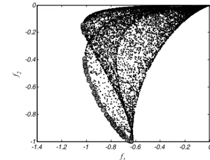
To find the non-dominated points, the Pareto dominance concept was applied to 5,000 randomly generated points over the interval(x1,x2)∈ [−4,4]. The approximation of the Pareto set and the
Figure 4– Nominal approximations of the Pareto set and Pareto front for minimization of the exponential functions f1(x1,x2)and f2(x1,x2).
To search robust solutions, the authors applied the robust multi-objective optimization procedure by adding the robustness index, as defined by Eq. (7), as a third objective function. The robust problem can be written as
minimize: f1(x1,x2)=c(−2,2)+c(2,2)+c(0,−2) and (9a)
f2(x1,x2)=c(0,0); and (9b)
f3(x1,x2)=R(x1,x2)=σmax (9c)
with c(a,b)= −exp −
x
1−a
2
2
−
x
2−b
2
2!
(9d)
The non-dominated points are shown in Figure 5. Clouds of points lie both near the nominal Pareto set and far away from it. In the specific problem, both functions are nearly flat in those regions. Accordingly, the robustness indexes for these points are very low, placing them as non-dominated although their function values are non-optimal compared to those near the nominal Pareto set.
Given the flat regions in Figure 3, one can conclude that the robustness index, when included in the multi-objective optimization problem as an additional objective function to be minimized, permits the location of the less sensitive non-dominated alternatives. Moreover, it naturally dis-perses the nominal Pareto front of the original problem, causing the decision-making process to become even more difficult.
Figure 5– Non-dominated alternatives for the multi-objective robust optimization problem of the exponen-tial functions f1(x1,x2), and f2(x1,x2)and the robustness indexR(x1,x2).
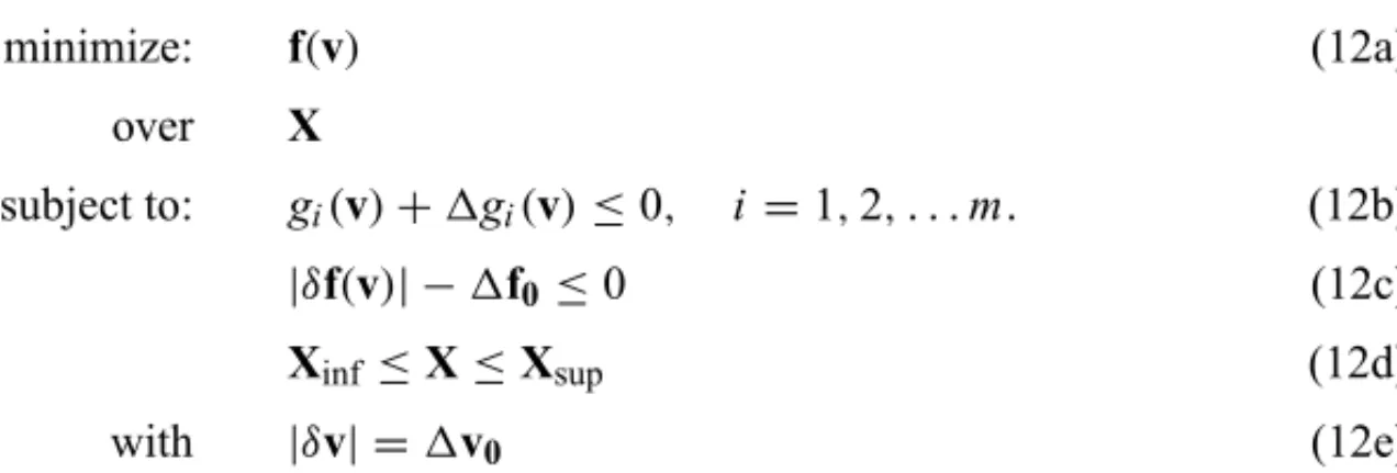
3.2 Optimum with acceptable variations in the objective function
To use this approach, the designer should know the bounds of variations in the design variables and in the design parameters, which are
|δv| =1v0 (10)
The designer also accepts a tolerance for the variations in the objective functions, which are
|δf|acc=1f0 (11)
minimize: f(v) (12a)
over X
subject to: gi(v)+1gi(v)≤0, i=1,2, . . .m. (12b)
|δf(v)| −1f0≤0 (12c)
Xinf≤X≤Xsup (12d)
with |δv| =1v0 (12e)
By using this approach, one can state the optimization problem with two exponential objective functions as:
minimize: f1(x1,x2)=c(−2,2)+c(2,2)+c(0,−2) and (13a)
f2(x1,x2)=c(0,0) (13b)
subject to: |δ(x1,x2)| −1f10≤0 (13c)
|δf2(x1,x2)| −1f20 ≤0 (13d)
1(x1,x2)0=0.1 (13e)
with c(a,b)= −exp −
x1−a
2
2
−
x2−b
2
2!
(13f)
where the acceptable function variations are set to 1 percent without loss of generality, and they include variations in the design variables that are equal to 10 percent of their nominal value. Figure 6 shows the Pareto optimal solutions plotted in the design space and the Pareto front approximation obtained by using the random walk over the design space.
Considering the acceptable values used, the robust Pareto front is less performing than the nom-inal one.
In the classical sensitivity analysis, the problems may have data (p, in the present notation) that are not specified exactly and are only known to belong to a given uncertainty set.
With the proposed methods, one can approach the engineering design optimization problem while considering the effects of uncertainty. The idea behind these methods is to consider that some data relating to engineering problems have variations around their nominal values. More-over, the problems’ data cannot be implemented exactly even if the data are certain and an optimal solutionX∗can be computed exactly.
4 APPLICATIONS
Figure 6– Non-dominated points for the robust multi-objective optimization problem of the exponential objective functions f1(x1,x2), and f2(x1,x2)with1(x1,x2)0=0.1 and1f10=1f20=0.01.
It contains six design variables, 21 constraints and three uncontrollable parameters, and it repre-sents a more realistic problem that naval architects are likely to face.
To solve both problems, one will need a method to find the Pareto front for multiobjective op-timization problems. The most widespread method in the literature is the genetic algorithm. Originally proposed by Holland (1975) for applications engaged with control theories, it was accepted quickly into numerous areas of engineering and science. Coello (2010) maintains an updated list of publications involving the genetic algorithm.
Many versions of genetic algorithms have served as meta-algorithms in the literature. The one that appears in this work was adapted from Debet al.(2000), which is the Non-dominated Sort-ing Genetic Algorithm, version II (NSGA II). This version is easy to use and depends on only two parameters: the number of chromosomes in the population and the number of generations that this population will evolve. With each evolution, the non-dominated solutions in the population converge toward the Pareto optimal solutions.
4.1 Problem 1: design of a vibrating platform
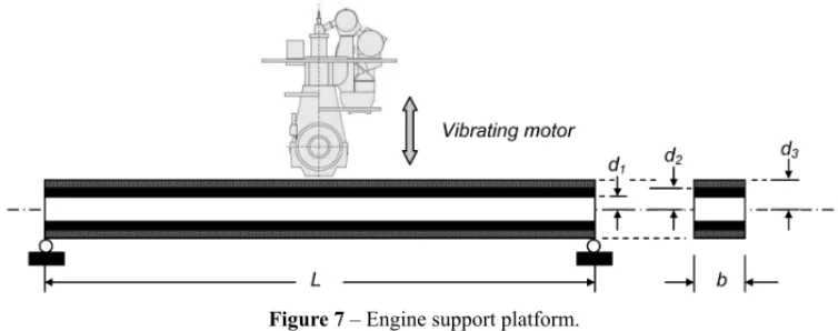
To illustrate the proposed robust approach, the authors present the engineering problem adapted from Gunawan and Azarm (2005).
Figure 7– Engine support platform.
The properties of the materials are shown in Table T1. In this table,ρis the mass density, Eis Young’s modulus and c is the material cost per volume. The objectives are to minimize the total material cost used in such a platform and to maximize its natural frequency by controlling five sizing variables (continuous) and one combinatorial variable (discrete). The sizing variables are the width of the platform(b), the length of the beam(L)and the thicknesses of the three layers (d1,d2andd3). The thicknesses of the middle and outer layers are represented as the difference
between two sizing variables (e.g., the thickness of the middle layer is equal to (d2−d1)).
The combinatorial variable is the choice of materials for the layers (M). Since there are three possible material types, there are six possibilities for M (starting from the inner layer outward): {A,B,C},{A,C,B},{B,A,C},{B,C,A}, {C,A,B}and{C,B,A}. The platform design is subjected to five constraints: the maximum weight of the platform and the lower and upper limits on the thickness of the middle and outer layers. The optimization formulation for this example is shown in Eq. (14). The notations(ρ1, ρ2, ρ3),(E1,E2,E3)and(c1,c2,c3)refer to
the density, Young’s modulus and the material cost for the inner, middle and outer layers of the platform, respectively. The lower and upper bounds for the sizing variables are 0.05≤d1≤0.5,
0.2≤d2≤0.5, 0.2≤d3≤0.6, 0.35≤b≤0.5 and 3≤L ≤6.
maximize: fn=
π 2L2
s E I
μ (14a)
minimize: cost=2bL
c1d1+c2(d2−d1)+c3(d3−d2) (14b)
subject to: g1=μL−2800≤0 (14c)
g2=d1−d2≤0 (14d)
g3=d2−d1−0.15≤0 (14e)
g4=d2−d3≤0 (14f)
g5=d3−d2−0.01≤0 (14g)
with E I = 2b 3
E1d13+E2 d23−d13
+E3 d33−d23
(14h)
μ=2b
Table T1– Properties of the beam materials.
Material A Material B Material C
ρ kg/m3
100.0 2770 7780
E(G Pa) 1.6 70 200
cm3
500.0 1500 800
It is assumed that there are uncontrollable variations in the density of material A(ρA)and cost of
material B(cB), and the optimum solutions must be as minimally sensitive as possible to these
variations. Moreover, the designer wants to obtain the robust Pareto solutions to this problem for the nominal parameter valuesρA=100 kg/m3andcB=1500 $/m3.
The variations in the parameters affect the two objective functions and the platform weight, and this effect is incorporated in the constraint functiong1. To take into account the feasibility of the
robust search process, the following constraint functions were added.
g6= |1cost| −1cost0≤0 (15a)
g7= |1f n| −1f n0≤0 (15b)
g8=g1+ |1g1| ≤0 (15c)
where, for the sensitivity requirements, the acceptable relative variations in objective functions 1f n0
fn and
1cost0
cost were arbitrarily set in the values shown in Figure 8 with maximum variation
for the parameters of material A defined by 1ρA
ρA =
1cA
cA = 0.05. The variation related to the
constraints expressed in Eqs. (15a-15c) were calculated for the extreme points of the interval composed by the parameter with its variation.
In Figures (8a-8b), the nominal Pareto set of the problem (without the uncontrollable variations) and the Pareto set obtained using the robust approach are displayed. When the robustness index is considered as the third objective function, the non-dominated points (square points) are dispersed over the function space, barely touching the nominal Pareto front. Therefore, the nominal Pareto front is not robust.
as shown in Figures (8c-8d). Finally, as long as the order of the material in the platform layers’ cross section is acting as a design variable, the robust Pareto fronts will exhibit the behavior shown in Figure 8c. The fronts with a relatively small variation in restrictive acceptable cost will fall in a better region than the fronts with more flexible bounds.
Figure 8– Nominal and robust Pareto fronts of the platform design problem.
Table T2– Statistics for design cases varying1fio/fiand material code as free design variable.
dv→ b(m) L(m) d1(m) d2(m) d3(m) Material 1fn/fn(%) 1cost/cost(%) 1fio↓ b σb L σL d1 σd1 d2 σd2 d3 σd3 code
∗
1fn σ1f n 1cost σ1cost
nominal 0.35 2% 3.00 0% 0.33 29% 0.35 30% 0.35 31% 2 0.55 0.48 4.51 0.21
1% 0.35 0% 3.00 0% 0.17 44% 0.28 17% 0.28 17% 4 0.00 0.00 0.00 0.00
2% 0.35 0% 3.00 0% 0.23 56% 0.30 23% 0.31 23% 3 0.05 0.06 0.80 0.82
3% 0.35 0% 3.00 0% 0.18 59% 0.26 17% 0.27 17% 3 0.08 0.08 1.09 0.99
4% 0.35 0% 3.00 0% 0.25 17% 0.28 16% 0.28 17% 2 0.20 0.02 3.99 0.01
Furthermore, the proposed sensitivity approach is useful for characterizing robust Pareto fronts. With this approach, one can easily achieve the robust Pareto front. This approach does not require stochastic treatment for obtaining the variations, and it does not need a probability distribution for the variations in the design variables and design parameters.
4.2 Problem 2: preliminary design of a bulk carrier
The second application of the developed methodology is the preliminary design of a bulk carrier. The design of a vessel is not a trivial task. For decades, this problem has been handled in two ways. Some designers have adjusted a known design so that it meets new requirements, and others have relied on simplified mathematical models controlled by an optimization algorithm, which allow them to obtain the optimal solution based on previously established technical or economic criteria.
This work considers the second alternative with the aid of the mathematical model for designing bulk carriers, which was developed by Pratyush and Yang (1998) and presented in detail in Au-gustoet al.(2012) study. The model comprises a set of functions that define the vessel attributes. These functions constrain the design variables of the objective functions to be optimized as well as the space of these design variables. These functions characterize the technical and economic performance of the ship and allow designers to evaluate each design alternative. The economic performance of the ship refers to its annual unitary transportation cost and its annual transported cargo, and the technical performance of the ship refers to the functions of the vessel’s design vari-ables, including length, beam, depth, draft, block coefficient and speed, which are respectively (L,B,D,T,CbandVK). Pratyush and Yang chose to minimize the annual transportation cost,
maximize the amount of annual cargo and minimize the vessel’s weight. The present work chose the optimization of the first two with no loss of generality. These two functions are conflicting, as shown in Figures 9 and 10.
The authors applied the proposed multiobjective robust optimization to the ship’s design in order to consider the isolated variation in each design variable and in each design parameter for the two approaches. First, the Robustness Index was added as a third objective function to the original bi-objective optimization problem. Then, the variations relative to the nominal value of the design variable and to the design parameter were arbitrarily preset at1xio =1 percent and 5 percent,
respectively, and the consequent variations of the objective functions were limited to1fio and
arbitrarily set at values ranging from 1 percent to 4 percent relative to their resultant or nominal values, depending on the case.
Figure 10 shows the results for robust optimization related to variations in the arbitrarily chosen design parameters, namelyround trip, fuel oil price andhandling rate, since they can affect negatively the performance functions, depending on the uncertainties of their nominal values.
Figure 10– Nominal and robust Pareto fronts for the minimization of transportation cost(C T)and maxi-mization of annual transported cargo(AC), allowing isolated variations in the design parameters of round trip, fuel oil price and handling rate.
Each figure shows the nominal (non-robust) Pareto front, the robust Pareto front considering the Robustness Index as the third objective function to be minimized and the Pareto front considering different levels of acceptable objective function variations due to an arbitrary parameter variation interval of1pio =5 percent around the parameter’s nominal value.
From both figures, it can be seen that variations in problem variables and problem parameters impact the extension and the performance of objective functions. More important is that the variation with the most impact in the nominal Pareto front is associated with thehandling rate
nominal value is set to 8,000 t/day, the nominal Pareto front is very sensitive. For acceptable levels of variations in objective functions over the interval1fio ∈ [1%,3%], the respective Pareto
fronts practically collapse to a single solution in each respective front. This single solution will be partially robust if the acceptable levels of variations are higher, namely 1fio = 4 percent,
when compared to those observed in the results obtained with uncontrollable variations in the design variables and other design parameters.
Therefore, this parameter plays an important role in the design process, because its impact on the objective functions can degrade drastically the performance of the designed ship.
5 CONCLUSIONS
Most engineering design problems are multiobjective and contain antagonistic objective func-tions. To solve such problems, many researchers developed methods that helped them to search for a general solution. They have frequently elected to use evolutionary methods to locate a set of solutions of multiobjective optimization problems. These algorithms provide a discrete picture of the Pareto front in the function space.
This paper introduced a new concept of a sensitivity index to perform multiobjective robust design optimizations, mainly when performance functions are highly sensitive to the variations in the design variables and in the design parameters.
To introduce the concept, the authors presented formulations of a multiobjective optimization problem, a robust design problem and a multiobjective robust optimization problem. A robust-ness index was introduced in order to classify the nominal Pareto front as either non-sensitive robust or not. This robustness index is based on the singular values of the sensitivity Jacobian matrix involving the objective functions, and it is considered an additional function to be mini-mized in the optimization problem. If the nominal Pareto front is not robust, then the new front, in view of the robustness index, will be scattered in the function space.
In addition, this paper proposed a supplementary method for searching for the robust Pareto front in instances where the design variables and design parameters have known uncontrollable variations bounded in single intervals and the designer will accept a range of these variations in the objective functions. During this search for optimal solutions, the designer constrains varia-tions in objective funcvaria-tions to the acceptable intervals. The feasibility of the nominal problem is maintained once the effects of the variations in the constraint functions are considered.
under design. Given the results of both illustrations, the proposed methodology appears to be a simple and useful tool for conducting robust engineering designs.
REFERENCES
[1] AUGUSTOO, BENNIS F & CAROS. 2012. A new method for decision making in multi-objective optimization problems.Pesquisa Operacional, in press.
[2] BEN-TAL A & NEMIROVSKI A. 1998. Robust convex optimization.Mathematics of Operations Research,23(4): 769–805.
[3] BEN-TAL A & NEMIROVSKI A. 2002. Robust optimization – Methodology and applications. Mathematical Programming,92(3): 453–480.
[4] BERTSIMASD, PACHAMANOVAD & SIMM. 2004. Robust linear optimization under general norms. Operations Research Letters,32: 510–516.
[5] BERTSIMASD & SIMM. 2004. The price of robustness.Operations Research,52(1): 35–53.
[6] CARO S, BINAUD N & WENGER P. 2008. Sensitivity analysis of planar parallel manipulators. Proceedings of ASME Design Engineering Technical Conferences, August 3-6, New York, NY, U.S.
[7] CHASEK, GAOJ, MAGLEBYSP & SORENSENCD. 1996. Including geometric feature variations in tolerance analysis of mechanical assemblies.IIE Transactions,28: 795–807.
[8] CHENW, ALLENJK, TSUIK-L & MISTREEF. 1996. A procedure for robust design: minimizing variations caused by noise factors and control factors.ASME Journal of Mechanical Design, 118: 478–485.
[9] COELLOCAC. 2010. List of references on evolutionary multiobjective optimization. http://www.lania.mx/∼ccoello/EMOO/EMOObib.html. Last accessed April 24, 2010.
[10] DEB K, AGRAWAL S, PRATAB A & MEYARIVAN T. 2000. A fast elitist non-dominated sorting genetic algorithm for multiobjective optimization. Technical Report 200001 NSGA-II, KanGAL.
[11] DEBK. 2001. Multiobjective Objective Optimization using Evolutionary Algorithms. San Francisco: Wiley & Sons, Ltd.
[12] GIASSI A, BENNIS F & MAISONNEUVE JJ. 2004. Multidisciplinary design optimization and robust design approaches applied to concurrent design. International Journal of Structural and Multidisciplinary Optimization, ISSMO,28: 356–371.
[13] GOLDBERG D. 1989. Genetic Algorithms in Search and Machine Learning. Reading: Addison Wesley.
[14] GUNAWAN S & AZARM S. 2005. Multiobjective robust optimization using a sensitivity region concept.Structural Multidisciplinary Optimization,29: 50–60.
[15] HOLLANDJ. 1975. Adaptation in Natural and Artificial Systems. Ann Arbor: University of Michigan Press.
[16] KALSIM, HACKERK & LEWISK. 2001. A comprehensive robust design approach for decision trade-offs in complex systems design.ASME Journal of Mechanical Design,121: 1–10.
[18] PARKINSONDB. 2000. The application of a robust design method to tolerancing.ASME Journal of Mechanical Design,22: 149–154.
[19] PRATYUSHS & YANGJB. 1998. Multiple Criteria Decision Support in Engineering Design. New York: Springer.
[20] SCHAFFERJD. 1985. Multiple objective optimization with vector evaluated genetic algorithms. In: Proceedings of the First International Conference on Genetic Algorithms and their Applications [edited by J.J. Grefenstette], Psychology Press, 93–100.
[21] SUNDARESANS, ISHIIK & HOUSERDR. 1993. A robust optimization procedure with variations on design variables and constraints.Advances in Design Automation,1: 379–386.