Submitted13 May 2016 Accepted 2 August 2016 Published8 September 2016
Corresponding author
Marco Basile, [email protected]
Academic editor Luis Eguiarte
Additional Information and Declarations can be found on page 14
DOI10.7717/peerj.2398
Copyright 2016 Basile et al.
Distributed under
Creative Commons CC-BY 4.0
OPEN ACCESS
Patchiness of forest landscape can
predict species distribution better than
abundance: the case of a forest-dwelling
passerine, the short-toed treecreeper, in
central Italy
Marco Basile1,2,3, Francesco Valerio4, Rosario Balestrieri1,2, Mario Posillico1,5, Rodolfo Bucci5, Tiziana Altea5, Bruno De Cinti1and Giorgio Matteucci6
1Istituto di Biologia Agroambientale e Forestale, Consiglio Nazionale delle Ricerche, Monterotondo Scalo, Italy 2Coordinamento MItO2000, Parma, Italy
3Chair of Wildlife Ecology and Management, Albert-Ludwigs-Universität Freiburg, Freiburg, Germany 4CIBIO/InBIO-UE—Research Center in Biodiversity and Genetic Resources, Pole of Évora Applied
Population and Community Ecology Laboratory, University of Évora UBC—Conservation Biology Lab, Department of Biology, Évora, Portugal
5Ufficio Territoriale Biodiversità di Castel di Sangro-Centro Ricerche Ambienti Montani, Corpo Forestale
dello Stato, Castel di Sangro, Italy
6Istituto per i Sistemi Agricoli e Forestali del Mediterraneo, Consiglio Nazionale delle Ricerche, Ercolano (Na),
Italy
ABSTRACT
values. The study lends support to the concept that the degree of fragmentation can contribute to alter not only the suitability of an area for a species, but also its abundance. Even if the relationship between suitability and abundance can be used as an early warning of habitat deterioration, its weak predictive power needs further research. However, we define relationships between a species and some landscape features (i.e., fragmentation, extensive rejuvenation of forests and tree plantations) which could be easily controlled by appropriate forest management planning to enhance environmental suitability, at least in an area possessing high conservation and biodiversity values.
SubjectsBiodiversity, Conservation Biology, Ecology
Keywords SDM, Quantile regression, Fragmentation, Management, Heterogeneity
INTRODUCTION
In recent years, considerable research effort has been involved in studying the influence of landscape patterns on biodiversity, triggered by the wide availability of biological data, as well as by the development of sophisticated species distribution models (SDMs), capable of predicting the presence of a species as a function of environmental variables (Elith & Leathwick, 2009). The reliability of SDMs is based on the quality of occurrence data and the use of environmental predictors linked to species occurrence (Austin, 2007). For instance, presence data collected through nationwide standardised monitoring programmes provide enormous advantages in using SDMs, due to the creation of large databases (Elith & Leathwick, 2009), hosting large amounts of occurrences and covering a wide, biologically significant area. Appropriate environmental predictors are those supposed to best describe the set of abiotic and biotic conditions affecting species occurrence, i.e., those characterising the species ecological niche (sensuHutchinson; Hutchinson, 1957;Holt, 2009). Indeed, large-scale species distribution modelling can be useful for addressing species-habitat relationships at multiple spatial scales in order to understand the spatial variability in habitat selection (Farashi, Kaboli & Karami, 2013;Chefaoui et al., 2015;Morand et al., 2015). Also, considering the spatial heterogeneity in the environment has become essential in many studies regarding reproduction, meta-population dynamics, gene flow, dispersal and connectivity (Bender, Tischendorf & Fahrig, 2003;Wang et al., 2008;Ryberg et al., 2013). Recent studies have addressed this issue to propose alternative conservation strategies (Nixon et al., 2014), to monitor landscape change (Darvishi, Fakheran & Soffianian, 2015) and to give insight into the distribution of native and non-native species (Kumar, Stohlgren & Chong, 2006). Moreover, spatial patterns are considered major drivers of many ecosystem processes (Uuemaa, Mander & Marja, 2013).
the biological community, or biotic homogenisation across the landscape (McKinney & Lockwood, 1999). Such a consequence derives from the loss of unique habitats, which are not replaceable in the short term (Fahrig, 2003).
Species abundance is also influenced by spatial variability, being affected by spatial gradi-ents in the environmental parameters that form the environmental niche (Martínez-Meyer et al., 2013). Optimal conditions can be found where the environmental parameters are close to the centroid of the Hutchinsonian niche (Hutchinson, 1957). Hence, environmental variability can influence both the presence and abundance of a species. Indeed, the decrease in abundance could warn about a species decline in population and/or range extent earlier than a decrease in environmental suitability. In fact, abundance could also be low in highly suitable regions, in response to local limiting factors (VanDerWal et al., 2009). The aim of our study was to investigate the relationship between environmental suitability and abundance of a species, in response to fragmentation. However, true envi-ronmental suitability can be expressed only by the whole set of envienvi-ronmental predictors and the local conditions that can influence movements and interaction (Grinnell, 1917) and the persistence of those conditions itself (Jackson & Overpeck, 2000). Such an approach may be unfeasible, as in our case. Therefore, we refer to a restricted set of factors influencing local or regional environmental suitability, i.e., some environmental predictors, which are supposed to be related to the probability of occurrence, and concern habitat suitability (HS) (Franklin, 2009). Among those habitats that can be highly modified by human activities, our research focused on forests, where unsustainable timber harvest can result in a patchy landscape and alter the habitat, adversely affecting forest biodiversity (Donald et al., 1998;
Penman, Mahony & Lemckert, 2005; Craig, 2007; Bearer et al., 2008; Shifley et al., 2008;
Czeszczewik et al., 2014;Calladine et al., 2015;Escobar et al., 2015). Woody plants are key elements in shaping the distribution of several bird speciessuch asbirds (MacArthur, Recher & Cody, 1966;Cody, 1985). Landscape structures and the spatial arrangement of habitat patches can affect both the abundance and distribution of birds, acting as structural bio-modifiers (Uuemaa, Mander & Marja, 2013).
modelled HS with several algorithms and compared results, to assess whether different species distribution models (SDMs) follow the same pattern of response.
METHODS
One of the main advantages offered by SDMs relies on the use of occurrence data collected with different methods (Tsoar et al., 2007). Therefore we used occurrence records from multiple sources, that spanned from year 2000 to 2013. We relied mainly on the MITO2000 database (Monitoraggio Italiano Ornitologico, Italian Ornithological Monitoring), an ongoing project which started in 2000 and operates at a country-wide level (Fornasari et al., 2010). The project uses point counts with unlimited radius (Blondel, Ferry & Frochot, 1981), sampling points being randomly selected within a 1 km2grid square in the region
of interest. Point counts were carried out during a short time frame, from mid-May to mid-June. Occurrences ofC. brachydactylawere also extracted from the databases of the National Forest Service (Ufficio Territoriale della Biodiversità, Castel di Sangro, AQ), and the LIFE+ManFor C.BD project, which employed a sampling design similar to MITO2000,
albeit at a smaller spatial scale (∼200–500 m). The spatial coverage of the occurrences was
limited to the administrative boundaries of the regions of Lazio, Abruzzo and Molise, comprising 32,523 km2, of which over one-third (12,309 km2) had forest cover (Fig. 1).
The whole database was filtered from all the pseudo-replicated points that fell into the same 1 km2grid. The database was further cleared of all the occurrences that were located
in unrealistic locations (i.e., non-forested areas), except for those <300 m away from the nearest forest patch, which were relocated to the nearest patch. Every occurrence was georeferenced with GPS. Hence, for our purposes, the error in location was assumed to be the same across the three datasets. The final database consisted of 170 occurrence points of C. brachydactyla(Table 1), of which 119 were supplied by the MITO2000 database, exceeding the recommended minimum sample size (Wisz et al., 2008).
Species distribution models
The SDMs were implemented using five environmental predictors, correlated with forest structure, productivity and the degree of fragmentation, at a spatial resolution of 30 m. First, a habitat type map, consisting of 12 classes, was created from the regional forest maps (Marchetti, Chiavetta & Santopuoli, 2009;Garfí & Marchetti, 2011;Open Data Lazio, 2012), aggregating all of the non-forest habitat and distinguishing 11 forest types (Table 1). Three landscape metrics were then calculated from the habitat map, using FRAGSTATS v. 4 software (McGarigal, Cushman & Ene, 2012): (1)Diversity (H’), a measure of patch type diversity within the landscape (Shannon & Wiener, 1949); (2)edge density(ED) which expresses the density (m ha−1) of boundaries; (3) theaggregation index(AI) which measures
Figure 1 Treecreeper’s occurrences used to build the distribution models.The study area is located in central-southern Italy, within Abruzzo, Lazio and Molise regions.
Table 1 Surface of the habitat types included in the analysis within the study area (Abruzzo, Lazione and Molise regions, central Italy) and number of short-toed treecreeper’s occurrences.
Forests and tree plantations habitat types Area (km2) N◦of treecreeper’s occurrences
Holm oak (Quercus ilex) 511.9 8
Downy oak (Q. pubescens) 1986.3 13
Turkey oak (Q. cerris) 2412.3 51
Orno-ostryetum(mixed deciduous woodland with prevailingFraxinus ornusandOstrya carpinifolia)
1342.4 20
Chestnut (Castanea sativa) 628.1 10
Tilio-Acerion 0.12 0
Beech (Fagus sylvatica) 2360.4 40
Salixsp. andPopulussp. riparian woodlands and poplar plantations
536.5 12
Tree plantations and bushes 649.7 8
Conifer (both natural and reforestation) 545 4
Shrubland and maquis 1313.1 4
Non forest 20129.3 0
spatial resolution. NDVI was computed over a mosaic of five images with cloud cover <10%, collected between July and August 2013, which had undergone the atmospheric correction procedure. Finally, altitude was integrated through a digital elevation model (DEM) provided by the National Institute for Environmental Protection and Research (ISPRA), available athttp://www.sinanet.isprambiente.it/it.
Spatial autocorrelations of the environmental predictors within occurrence points were tested through a Mantel test in order to detect any spatial autocorrelations among occurrences (Fig. S1). Analyses were carried out with the R package ‘ecospat’ (Broennimann, Di Cola & Guisan, 2016).
Among the eight selected algorithms, the maximum entropy (ME) used presence-only points in combination with background samples, using presence-only quadratic and hinge features to avoid overfitting (Phillips, Anderson & Schapire, 2006;Elith et al., 2011). The other algorithms, which were supplied with pseudo-absences and true absences, were: an artificial neural network (ANN;Segurado & Araujo, 2004), classification tree analyses (CTA;
Breiman et al., 1984;De’ath, 2002), flexible discriminant analyses (FDA;Hastie, Tibshirani & Buja, 1994), generalized boosting model (GBM;Friedman, 2001), generalized linear model (GLM;McCullagh & Nelder, 1989), multivariate additive regression spline (MARS;
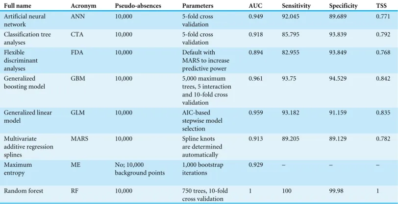
Moisen & Frescino, 2002) and random forest (RF;Breiman, 2001) (Table 2). Ten thousand absence points were sampled in the environmental background (Elith et al., 2006), comprising 975 points of actual absence derived from the MITO2000 database and 9025 pseudo-absences, randomly selected within the area where the logistic output of ME was less than 0.2 (Chefaoui & Lobo, 2008;Wisz & Guisan, 2009), representing an adequate number of pseudo-absences (Barbet-Massin et al., 2012). SDMs were trained using 70% of randomly selected occurrences, while the remaining 30% were used for testing; the procedure was iterated 30 times (except for ME with 50 iterations) (further details are provided inTable 2). The area under the curve (AUC) of the receiving operating characteristic (Hanley & McNeil, 1982) was used to evaluate the predictive power of the SDMs. To improve the readability of SDM outputs, sensitivity (i.e., the proportions of correct positive prediction) and specificity (i.e., the proportion of correct negative prediction) and the true skill statistic (TSS) were also reported (Allouche, Tsoar & Kadmon, 2006;Lobo, Jiménez-Valverde & Real, 2008). The importance of each environmental predictor was calculated followingThuiller et al. (2009). Analyses were carried out with the software MaxEnt (Phillips, Anderson & Schapire, 2006) and thebiomod2package integrated in R (Thuiller et al., 2009;R Development Core Team, 2015;Thuiller, Georges & Engler, 2015).
Abundance estimation
Abundance was estimated in two forest stands used as test sites of the LIFE+ManFor
C.BD: Bosco Pennataro Regional Forest and Chiarano-Sparvera Regional Forest. Bosco Pennataro (BP, 41◦44′N, 14◦11′E, 1,000 m a.s.l.) consists of a multi-layered high forest
stand dominated by turkey oak (Quercus cerris). Chiarano-Sparvera (CS, 41◦51′N, 13◦57′E,
1,700 m a.s.l.) is a pure beech (Fagus sylvatica) forest, in transition from coppice to high forest. Following a systematic design, 27 and 23 sampling points, 125.5 m (±19.7 sd) away
Table 2 Settings used for species distribution modelling and resulted AUC (area under the curve of the receiving operator characteristic), sen-sitivity, specificity and TSS (true skills statistic).
Full name Acronym Pseudo-absences Parameters AUC Sensitivity Specificity TSS
Artificial neural network
ANN 10,000 5-fold cross
validation
0.949 92.045 89.689 0.771
Classification tree analyses
CTA 10,000 5-fold cross
validation
0.918 85.795 93.839 0.792
Flexible discriminant analyses
FDA 10,000 Default with
MARS to increase predictive power
0.894 82.955 93.849 0.768
Generalized boosting model
GBM 10,000 5,000 maximum
trees, 5 interaction and 10-fold cross validation
0.961 93.75 94.529 0.842
Generalized linear model
GLM 10,000 AIC-based
stepwise model selection
0.959 93.182 91.159 0.835
Multivariate additive regression splines
MARS 10,000 Spline knots
are determined automatically
0.913 89.205 89.129 0.782
Maximum entropy
ME No; 10,000
background points
1,000 bootstrap iterations
0.929 – – –
Random forest RF 10,000 750 trees, 10-fold
cross validation
1 100 99.98 1
May to June (2012 in CS; 2013 in BP) from sunrise till 11:00 a.m. At every point, each individual detected by aural/visual cues during a five-minute count was recorded. Each point was visited two to six times (average=3.4; total=177).
Local abundance was estimated with N-mixture models (Royle, 2004b). This approach considers local abundance (i.e., abundance estimated in each sampling point) as an independent random point process (Royle, 2004a). Two separate models were built for BP and CS, respectively: with and without detectability variation among occasions. Model fit and overdispersion (also called c-hat) was tested through a Pearsonχ2goodness-of-fit test, with 1,000 bootstrap resampling (MacKenzie & Bailey, 2004). Model selection proceeded through Akaike’s Information Criterion, which assigns scores both to the likelihood of the model and the number of parameters included (Burnham & Anderson, 2002). Spatial dependence of estimates was assessed with the Moran test and index calculation (Moran, 1950). Analyses were carried out using the packagesunmarked (Fiske & Chandler, 2011),
AICmodavg (Mazerolle, 2015) andspdep (Bivand & Piras, 2015) implemented in R (R Development Core Team, 2015).
Statistical analyses
transforming the estimated population size (i.e., the sum of local abundances) into densities (ind./ha): the area of interest for density transformation was given by the minimum convex polygon among the sampling points. The difference between BP and CS environmental suitability values was tested by anF-test and at-test. The landscape metric values were also tested for difference with the same methods.
The relationship between abundance and environmental suitability can form a triangular envelope, where increasing values of environmental suitability are matched by increasing values of the maximum abundance, not just the mean abundance (VanDerWal et al., 2009). Therefore, quantile regression can best provide the opportunity to explore the relation between environmental suitability and the upper quantiles of the abundance (Cade, Noon & Flather, 2005). The triangular envelope can predict maximum abundance, given a suitability value, due to the increase in the slope of regressions of upper quantiles, while intercepts remain similar (VanDerWal et al., 2009). However, two factors can mask the results: first, random variation at every point also due to local limiting factors that are not feasible to model; secondly, the spatial structure of the data, that can generate autocorrelation. Therefore, quantile mixed regressions were implemented to model the abundance as a function of HS values of every SDM, with a null random term and a grouping factor identifying the two locations. The random effect is estimated through best linear prediction (Geraci & Bottai, 2013). Model fit was assessed for every quantile through comparison of AIC scores with the null model of the corresponding quantile (Burnham & Anderson, 2002). Statistical analysis was carried out with thelqmmpackage (Geraci, 2014) in R (R Development Core Team, 2015).
RESULTS
Each SDM showed an AUC >0.9, except for FDA (Table 2). Among them, RF ranked the highest value (AUC=1). However, the geographical projections of the SDMs proved
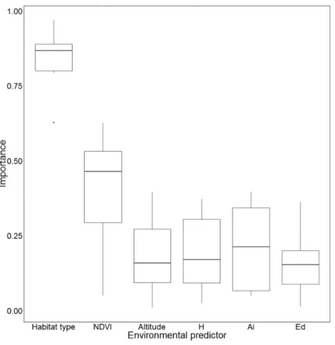
dissimilar (see Fig. S2). The importance of each environmental predictor had the same pattern for every algorithm, with forest type and NDVI proving the most important (Fig. 2). The importance of the three landscape metrics (H, AI, ED) indicates that the spatial configuration of landscape structures exerts a major influence on potential distribution.
Abundance models that performed best in both study areas were those in which detectability was invariant between sessions. Detectability was 0.34 (±0.11 SE) in Bosco
Pen-nataro and 0.21 (±0.27 SE) in Chiarano Sparvera. Local abundances significantly differed
between the two areas (F=0.77,p=0.53;t= −3.57,p<0.001), and mean estimates were 1.54 (±0.52 SE) in BP and 0.86 (±1 SE) individuals/point in CS. Both models returned a
good fit, with no overdispersion (BP:χ2=64.3,p=0.997, c-hat=0.687; CS:χ2=52.5,
p=0.391, c-hat=1). Estimates did not show spatial autocorrelation in the two forest stands, obtaining a Moran I of 0.11 (p=0.14) and−0.26 (p=0.92) for BP and CS, respectively.
Figure 2 Variable importance based on different Species Distribution Models (SDMs).NDVI, Nor-malized difference vegetation index; H’, Shannon index computed on landscape patch type diversity; Ai, aggregation index of landscape patches; Ed, patches’ edge density.
equally distributed among types (H’ =0.93), compared to CS (AI =92.6; H’=0.76).
Hence, landscape metrics showed a more fragmented landscape in CS than in BP, as expected.
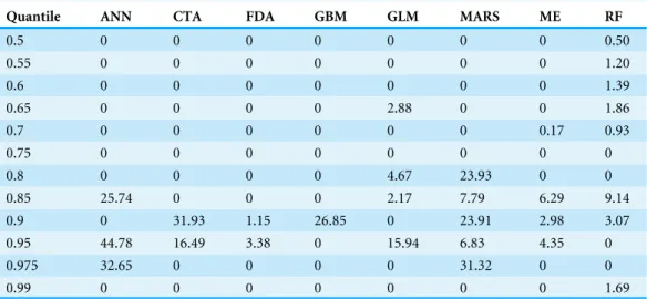
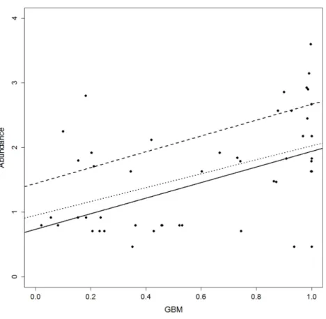
Quantile regression showed a positive relationship between abundance and HS (Fig. 3andFig. S3). No differences emerged for the regression slope of each quantile, while intercept values proved more variable. Moreover, the majority of slopes were not significant except for CTA, GBM and GLM (seeTable S1), even if AIC comparison indicated that most of the quantiles performed better than the corresponding null model (Table 4).
DISCUSSION
Table 3 Test for differences of landscape metrics and environmental suitability between Bosco Pen-nataro and Chiarano-Sparvera, based on Species Distribution Models (SDMs).
F P t p
Metric
H’ 0.065 0.000 3.3342 0.0027
Ed 0.3583 0.0134 −1.5038 0.1392
Ai 0.221 0.000 7.1504 0.000
Model
ANN 0.07 0.000 −36 0.000
CTA 4.901 0.000 −9.93 0.000
FDA 2433.4 0.000 −8.06 0.000
GBM 1.137 0.748 −10.91 0.000
GLM 2.996 0.008 −2.949 0.002
MARS 14648 0.000 −4.893 0.000
ME 46.35 0.000 −4.682 0.000
RF 30.42 0.000 −4.044 0.000
Notes.
H’, Shannon index of patch type diversity; Ed, edge density; Ai, aggregation index;F, Fisher’s test;t,ttest;P,pvalue; model abbreviation are given inTable 2.
Table 4 DeltaAIC between null model and suitability-dependant model, for the same quantile.
Quantile ANN CTA FDA GBM GLM MARS ME RF
0.5 0 0 0 0 0 0 0 0.50
0.55 0 0 0 0 0 0 0 1.20
0.6 0 0 0 0 0 0 0 1.39
0.65 0 0 0 0 2.88 0 0 1.86
0.7 0 0 0 0 0 0 0.17 0.93
0.75 0 0 0 0 0 0 0 0
0.8 0 0 0 0 4.67 23.93 0 0
0.85 25.74 0 0 0 2.17 7.79 6.29 9.14
0.9 0 31.93 1.15 26.85 0 23.91 2.98 3.07
0.95 44.78 16.49 3.38 0 15.94 6.83 4.35 0
0.975 32.65 0 0 0 0 31.32 0 0
0.99 0 0 0 0 0 0 0 1.69
Figure 3 Scatterplot of abundance versus habitat suitability (as predicted by the Generalised Boosting model, GBM).Regression lines represent the fitted relationship at different quantiles. Quantiles: solid line =0.5 quantile, slope=0.37,p<0.5; dashed line=0.75, slope=0.19,p=n.s.; dotted line=0.95, slope
=0.13,p=n.s.
predictability of SDMs (Austin, 2007;Lobo, Jiménez-Valverde & Real, 2008). Specifically, the AUC does not consider the goodness of fit of a model and it is higher when more pseudo-absences in unsuitable localities are included in the model (Lobo, Jiménez-Valverde & Real, 2008). Nevertheless, its use is still widespread (Elith & Graham, 2009;Barbet-Massin et al., 2012). It should also be pointed out that, even if we used a large number of (pseudo) absences, we also employed a larger number of presence points than what is usually found in the literature (e.g.,Pearson et al., 2007).
assume that the variability in detectability is reduced to the minimum, demonstrating this issue also in the two forests where we estimated abundance (i.e., BP and CS). Finally, our use of the logistic output of ME, as well as of its subjective intercept of 0.5, is based upon the consideration that 37% of the study area is covered in forest. Therefore, assuming an intercept of 0.5 does not seem too far from reality scenario. Indeed, ME has been proved to be one of the most reliable SDMs when only presence data are available (Franklin, 2009;Merow, Smith & Silander, 2013). Our use of ME, moreover, was functional to the selection of pseudo-absences, which were not selected within the entire region, but only in a restricted area considered unsuitable by ME. As a consequence, we also assume that our method of selecting pseudo-absence greatly reduced an eventual bias. At the very end, we considered SDM outputs as a habitat suitability index, which we could assume to be related to actual environmental suitability (VanDerWal et al., 2009;Brambilla & Ficetola, 2012).
For reliable modelling, it is necessary to use ecologically relevant environmental predictors (Austin, 2007), even if it is not possible to include every environmental variable thought to affect the distribution of a species (Elith & Leathwick, 2009). We based the choice of environmental variables on both the known species-habitat relationships and on the possibility of obtaining relevant information to steer management, relying on forest type, structure, productivity and fragmentation. Forest type and NDVI proved the most impor-tant variables in predicting the distribution of the short-toed treecreeper. The NDVI is not only positively correlated to net primary productivity (Myneni et al., 1995;Pettorelli et al., 2005), but also to the structural complexity of forests (Manes et al., 2010). As a consequence, among the same forest type, a higher NDVI is related, given that all other variables are comparable, to more structured, multi-layered forests or to forest patches that are more productive or that have a higher leaf area index, where specialist birds can find a more suitable habitat (Newton, 1994;Carrillo-Rubio et al., 2014). Obviously, this conclusion also depends on the patch size and the degree of fragmentation, which are intertwined with NDVI and forest type. Indeed, a substantial influence of landscape structure in defining habitat suitability was clearly apparent when taking into account the three metrics together. Responses to fragmentation are species-specific and, usually, the more specialist a species, the more negative its response (Devictor, Julliard & Jiguet, 2008;Rueda et al., 2013). SDM outputs showed higher HS in localities in less fragmented landscapes, in agreement with the literature on forest specialist birds (Fahrig, 2003).
We used hierarchical statistical analysis of abundance to obtain unbiased estimates, corrected for detectability (Royle, 2004a). The significant difference in abundances between Bosco Pennataro and Chiarano-Sparvera is matched by the difference in the suitability of the two forests. Therefore, differences in abundance, HS and landscape metrics matched the same pattern: in locations with more degraded forest, both HS and abundance scored lower values, even though abundance showed higher variability, confounding the hypothesised relationships with HS.
for the relationship between demographic parameters and HS (Pearce & Ferrier, 2001;
Nielsen et al., 2005;Jiménez-Valverde et al., 2009). Related findings are often discordant (Jiménez-Valverde et al., 2009;Tôrres et al., 2012) and many concerns are raised on the controversial and often unconfirmed empirical relationships between ecological processes and landscape patterns (Turner, Gardner & O’Neill, 2001;Kupfer, 2012). That said, the rela-tionship can be masked by the many unmodelled environmental variables that can conceal local suitability (Lobo, Jiménez-Valverde & Real, 2008). For this reason,VanDerWal et al. (2009) concluded that just the upper limit of abundance, and not its mean value, is predictable from HS. However, this relationship has been widely found to be very weak due to the difficulty to obtain reliable estimates of both abundance and HS (Jiménez-Valverde, 2011;Oliver et al., 2012;Tôrres et al., 2012). Some exceptions are presumably due to the use of indexes of abundance, instead of actual estimates (De Moraes Weber & Viveiros Grelle, 2012; Gutiérrez et al., 2013). Indeed, our approach was based not only on abundance estimates but also on HS values from different algorithms and averaged over the likely home range size. Moreover, our use of landscape features as predictive variables could have enhanced model performance since other studies (e.g.,Tôrres et al., 2012), based mostly on climatic variables, found positive but weaker relationships between HS and abundance.
This result, though confirming the existence of a relationship, also highlights the limits of the SDM approach, suggesting that low HS can also occur in areas of high abundance, probably due to environmental factors that are not considered in modelling which may increase the actual HS of the area.
CONCLUSION
Birds are considered good biodiversity indicators, especially to monitor habitat alteration (e.g., fragmentation) (Gregory et al., 2008;Carrillo-Rubio et al., 2014;Czeszczewik et al., 2014). For instance, in the context of biotic homogenization, one likely effect is the disappearance of specialist species which are more closely associated to unaltered forests (McKinney & Lockwood, 1999). Negative effects of habitat alteration can persist over years (Kendrick et al., 2014). Thus identification of the main species-habitat relationships is important to prevent the disappearance of more susceptible species (Villard, Trzcinski & Merriam, 1999;King & DeGraaf, 2000). Further, fragmentation can cause the disappearance of the specialist component of biodiversity (Fahrig, 2003). Such processes can alter biolog-ical, ecological and demographic traits like brood survival and growth (Suorsa et al., 2003;
Le Tortorec et al., 2012), occupancy or population size (Schmiegelow, Machtans & Hannon, 1997; Villard, Trzcinski & Merriam, 1999; Cooper & Walters, 2002). Through SDMs, such results can be transposed into geographic projection and inform conservationists and practitioners (Ferrier et al., 2007;Maiorano et al., 2015). Therefore, modelling how fragmentation can affect the distribution of a species and understand the eventual relations with population decrease, can greatly improve conservation and management plans.
In this way, we define the relationships between a species and some ‘‘directly adjustable’’ landscape features. The Chiarano-Sparvera forest stand is naturally located in a more fragmented landscape than is Bosco Pennataro. Hence, the abundance response (i.e., decrease) of the short-toed treecreeper is matched by habitat choice. Fragmentation, extensive rejuvenation of forest stands and tree plantations are all factors that can contribute to alter the suitability of an area. Since habitat alteration can decrease species abundance sooner than effectively reducing their geographic range (Shoo, Williams & Hero, 2005), identification of areas of low HS, where impact on abundance is more likely to cause local extinctions, could act as an early warning for species conservation. In our approach, these threats can occur on a large scale, can be related to possible changes in abundance and then used to inform practitioners and managers. Moreover, prediction of future land use scenarios can be implemented.
However, our results are a case study, limited to a single specialist species, strictly linked to mature well-preserved forests. This approach could be extended over different kinds of habitats and species, other than forests. Moreover, the modelling should be refined to include other potential resources and limiting factors, whether biotic or abiotic, in order to obtain more robust HS prediction (Guisan & Thuiller, 2005). The magnitude of the relationship between HS and abundance can then be used as a form of model validation (Lobo, Jiménez-Valverde & Real, 2008), thus helping to steer sound land use management and conservation planning.
ACKNOWLEDGEMENTS
We are grateful to Jorge Soberón for valuable advice on the manuscript. We are also grateful to an anonymous reviewer for good advices. We are grateful to the secretary of the project MITO2000, especially to Simonetta Cutini, who patiently organized part of the dataset. Thanks are also due to Andrea Mancinelli for having assisted in many ornithological surveys and, in general, to the staff of the Isernia and Castel di Sangro Ufficio Territoriale Biodiversità del Corpo Forestale dello Stato (National Forest Service) for their logistic support. We are most grateful to the association ARDEA (www.ardeaonlus.it) for supporting our field work with its large number of volunteers.
ADDITIONAL INFORMATION AND DECLARATIONS
Funding
This research is part of the Life+ ManFor C.BD. project and hence has been co funded by a LIFE09 ENV/IT/000078 grant. The funders had no role in study design, data collection and analysis, decision to publish, or preparation of the manuscript.
Grant Disclosures
Competing Interests
Marco Basile and Rosario Balestrieri declare that they have no competing interest in publishing this work as affiliated to the MItO2000 project.
The remaining authors declare there are no competing interests.
Author Contributions
• Marco Basile conceived and designed the experiments, performed the experiments,
analyzed the data, wrote the paper, prepared figures and/or tables.
• Francesco Valerio and Mario Posillico analyzed the data, prepared figures and/or tables,
reviewed drafts of the paper.
• Rosario Balestrieri conceived and designed the experiments, performed the experiments,
reviewed drafts of the paper.
• Rodolfo Bucci performed the experiments.
• Tiziana Altea and Bruno De Cinti commented on the manuscript.
• Giorgio Matteucci reviewed drafts of the paper.
Data Availability
The following information was supplied regarding data availability:
Basile M, Valerio F, Balestrieri R, Posillico M, Bucci R, Altea T, De Cinti B, Matteucci G. 2016. Patchiness of forest landscape can predict species distribution better than abundance: the case of a forest-dwelling passerine, the short-toed treecreeper, in central Italy. Mendeley Data. v2.
http://dx.doi.org/10.17632/p2z6rtcf8j.2.
Supplemental Information
Supplemental information for this article can be found online athttp://dx.doi.org/10.7717/ peerj.2398#supplemental-information.
REFERENCES
Allouche O, Tsoar A, Kadmon R. 2006.Assessing the accuracy of species distribution
models: prevalence, kappa and the true skill statistic (TSS).Journal of Applied Ecology
43:1223–1232DOI 10.1111/j.1365-2664.2006.01214.x.
Austin M. 2007.Species distribution models and ecological theory: a critical
as-sessment and some possible new approaches.Ecological Modelling 200:1–19 DOI 10.1016/j.ecolmodel.2006.07.005.
Barbet-Massin M, Jiguet F, Albert CH, Thuiller W. 2012.Selecting pseudo-absences
for species distribution models: how, where and how many?Methods in Ecology and Evolution3:327–338DOI 10.1111/j.2041-210X.2011.00172.x.
Bearer S, Linderman M, Huang J, An L, He G, Liu J. 2008.Effects of fuelwood
col-lection and timber harvesting on giant panda habitat use.Biological Conservation
141:385–393DOI 10.1016/j.biocon.2007.10.009.
Bender DJ, Tischendorf L, Fahrig L. 2003.Using patch isolation metrics to predict
BirdLife International. 2016.Certhia brachydactyla. IUCN Red List for birds.Available at
http:// www.birdlife.org/ datazone/ userfiles/ file/ Species/ erlob/ summarypdfs/ 22711249_
certhia_brachydactyla.pdf.
Bivand R, Piras G. 2015.Comparing implementations of estimation methods for spatial
econometrics.Journal of Statistical Software63(18):1–36.
Blondel J, Ferry C, Frochot B. 1981. Point counts with unlimited distance. In: Ralph
JC, Scott JM, eds.Estimating numbers of terrestrial birds. Asilomar: Studies in Avian Biology, 414–420.
Brambilla M, Ficetola GF. 2012.Species distribution models as a tool to estimate
reproductive parameters: a case study with a passerine bird species.Journal of Animal Ecology 81:781–787DOI 10.1111/j.1365-2656.2012.01970.x.
Breiman L. 2001.Random forests.Machine Learning 45:5–32
DOI 10.1023/A:1010933404324.
Breiman L, Friedman JH, Olshen RA, Stone CJ. 1984.Classification and regression tree.
Belmont: Wadsworth International Group.
Broennimann O, Di Cola V, Guisan A. 2016.ecospat: spatial ecology miscellaneous
methods. R package V 2.0.Available athttps:// cran.r-project.org/ web/ packages/ ecospat/.
Burnham KP, Anderson DR. 2002.Model selection and multimodal inference. New York:
Springer-Verlag.
Cade BS, Noon BR, Flather CH. 2005.Quantile regression reveals hidden bias and
uncertainty in habitat models.Ecology 86:786–800DOI 10.1890/04-0785.
Calladine J, Bray J, Broome A, Fuller RJ. 2015.Comparison of breeding bird
assem-blages in conifer plantations managed by continuous cover forestry and clearfelling.
Forest Ecology and Management 344:20–29DOI 10.1016/j.foreco.2015.02.017.
Carrillo-Rubio E, Kéry M, Morreale SJ, Sullivan PJ, Gardner B, Cooch EG, Lassoie
JP. 2014.Use of multispecies occupancy models to evaluate the response of bird
communities to forest degradation associated with logging.Conservation Biology
28:1034–44DOI 10.1111/cobi.12261.
Chefaoui RM, Assis J, Duarte CM, Serrão EA. 2015.Large-scale prediction of seagrass
distribution integrating landscape metrics and environmental factors: the case of Cymodocea nodosa (Mediterranean–Atlantic).Estuaries and Coasts39(1):123–127 DOI 10.1007/s12237-015-9966-y.
Chefaoui RM, Lobo JM. 2008.Assessing the effects of pseudo-absences on
pre-dictive distribution model performance.Ecological Modelling 210:478–486 DOI 10.1016/j.ecolmodel.2007.08.010.
Cody ML. 1985.Habitat selection in birds. Orlando: Academic Press.
Cooper CB, Walters JR. 2002.Independent effects of woodland loss and fragmentation
on Brown Treecreeper distribution.Biological Conservation105:1–10.
Craig MD. 2007.The short-term effects of edges created by forestry operations on
the bird community of the jarrah forest, south-western Australia.Austral Ecology
32:386–396DOI 10.1111/j.1442-9993.2007.01710.x.
Czeszczewik D, Zub K, Stanski T, Sahel M, Kapusta A, Walankiewicz W. 2014.Effects of forest management on bird assemblages in the Bialowieza Forest, Poland.
iForest—Biogeosciences and Forestry8(3):377–385DOI 10.3832/ifor1212-007.
Darvishi A, Fakheran S, Soffianian A. 2015.Monitoring landscape changes in Caucasian
black grouse (Tetrao mlokosiewiczi) habitat in Iran during the last two decades.
Environmental Monitoring and Assessment 187:443DOI 10.1007/s10661-015-4659-3.
De Moraes Weber M, Viveiros Grelle CE. 2012.Does environmental suitability explain
the relative abundance of the tailed tailless bat, Anoura caudifer?Natureza and Conserva¸cao10:221–227DOI 10.4322/natcon.2012.035.
De’ath G. 2002.Multivariate regression trees: a new technique for modeling
species-environment relationships.Ecology 83:1105–1117
DOI 10.1890/0012-9658(2002)083[1105:MRTANT]2.0.CO;2.
Devictor V, Julliard R, Jiguet F. 2008.Distribution of specialist and generalist species
along spatial gradients of habitat disturbance and fragmentation.Oikos117:507–514 DOI 10.1111/j.0030-1299.2008.16215.x.
Donald PF, Fuller RJ, Evans AD, Gough SJ. 1998.Effects of forest management
and grazing on breeding bird communities in plantations of broadleaved and coniferous trees in western England.Biological Conservation85:183–197 DOI 10.1016/S0006-3207(97)00114-6.
Elith J, Graham CH. 2009.Do they? How do they? WHY do they differ? On finding
reasons for differing performances of species distribution models.Ecography
32:66–77DOI 10.1111/j.1600-0587.2008.05505.x.
Elith J, Graham CH, Anderson RP, Dudik M, Ferrier S, Guisan A, Hijmans RJ, Huettmann F, Leathwick JR, Lehmann A, Li J, Lohmann LG, Loiselle BA, Manion G, Moritz C, Nakamura M, Nakazawa Y, Overton JMC, Peterson AT, Phillips SJ, Richardson K, Scachetti-Pereira R, Schapire RE, Soberon J,
Williams S, Wisz MS, Zimmermann NE. 2006.Novel methods improve
pre-diction of species’ distributions from occurrence data.Ecography29:129–151 DOI 10.1111/j.2006.0906-7590.04596.x.
Elith J, Leathwick JR. 2009.Species distribution models: ecological explanation and
pre-diction across space and time.Annual Review of Ecology, Evolution, and Systematics
40:677–697DOI 10.1146/annurev.ecolsys.110308.120159.
Elith J, Phillips SJ, Hastie T, Dudík M, Chee YE, Yates CJ. 2011.A statistical
explanation of MaxEnt for ecologists.Diversity and Distributions17:43–57 DOI 10.1111/j.1472-4642.2010.00725.x.
Escobar MAH, Uribe SV, Chiappe R, Estades CF. 2015.Effect of clearcutting
op-erations on the survival rate of a small mammal.PLoS ONE10:e0118883 DOI 10.1371/journal.pone.0118883.
Fahrig L. 2003.Effects of habitat fragmentation on biodiversity.Annual Review of
Farashi A, Kaboli M, Karami M. 2013.Predicting range expansion of invasive raccoons in northern Iran using ENFA model at two different scales.Ecological Informatics
15:96–102 DOI 10.1016/j.ecoinf.2013.01.001.
Ferrier S, Manion G, Elith J, Richardson K. 2007.Using generalized dissimilarity
mod-elling to analyse and predict patterns of beta diversity in regional biodiversity assess-ment.Diversity and Distributions13:252–264
DOI 10.1111/j.1472-4642.2007.00341.x.
Fiske IJ, Chandler RB. 2011.Unmarked: an R package for fitting hierarchical models
of wildlife occurrence and abundance.Journal of Statistical Software43:1–23 DOI 10.18637/jss.v043.i10.
Fornasari L, Londi G, Buvoli L, Tellini Florenzano G, La Gioia G, Pedrini P, Brichetti
P, De Carli E. 2010.Distribuzione geografica e ambientale degli uccelli comuni
nidificanti in Italia, 2000–2004 (dati del progetto MITO2000).Avocetta34:5–224.
Franklin J. 2009.Mapping species distributions: spatial inference and prediction.
Cam-bridge: Cambridge University Press.
Friedman JH. 2001.Greedy function approximation: a gradient boosting machine.The
Annals of Statistics29:1189–1232DOI 10.1214/aos/1013203451.
Garfí V, Marchetti M. 2011.Tipi forestali e preforestali della regione Molise. Alessandria: Edizioni dell’Orso S.r.l.
Geraci M. 2014.Linear quantile mixed models: the lqmm package for laplace quantile
regression.Journal of Statistical Software57:1–29DOI 10.18637/jss.v057.i13.
Geraci M, Bottai M. 2013.Linear quantile mixed models.Statistics and Computing
24:461–479DOI 10.1007/s11222-013-9381-9.
Gil-Tena A, Torras O, Saura S. 2008.Relationship between forest landscape structure
and avian species richness in NE Spain.Ardeola55:27–40.
Gregory RD, Vořišek P, Noble DG, Van Strien A, Klvaňová A, Eaton M, Gmelig
Meyling AW, Joys A, Foppen RPB, Burfield IJ. 2008.The generation and use of
bird population indicators in Europe.Bird Conservation International18:223–244 DOI 10.1017/S0959270908000312.
Grinnell J. 1917.The niche-relationships of the California thrasher.The Auk34:427–433
DOI 10.2307/4072271.
Guisan A, Thuiller W. 2005.Predicting species distribution: offering more than simple
habitat models.Ecology Letters8:993–1009DOI 10.1111/j.1461-0248.2005.00792.x.
Gutiérrez D, Harcourt J, Díez SB, Illán JG, Wilson RJ. 2013.Models of
presence-absence estimate abundance as well as (or even better than) models of abun-dance: the case of the butterfly Parnassius apollo.Landscape Ecology28:401–413 DOI 10.1007/s10980-013-9847-3.
Hanley J, McNeil B. 1982.The meaning and use of the area under a receiver operating
characteristic (ROC) curve.Radiology143:29–36 DOI 10.1148/radiology.143.1.7063747.
Hastie T, Tibshirani R, Buja A. 1994.Flexible discriminant analysis by
He HS, Dezonia BE, Mladenoff DJ. 2000.An aggregation index (AI) to quantify spatial patterns of landscapes.Landscape Ecology15:591–601
DOI 10.1023/A:1008102521322.
Holt RD. 2009.Bringing the Hutchinsonian niche into the 21st century: ecological and
evolutionary perspectives.Proceedings of the National Academy of Sciences of the United States of America106:19659–19665DOI 10.1073/pnas.0905137106.
Hutchinson GE. 1957.Concluding remarks.Cold Spring Harbor Symposia on
Quantita-tive Biology22:415–427DOI 10.1101/SQB.1957.022.01.039.
Jackson ST, Overpeck JT. 2000.Responses of plant populations and communities
to environmental changes of the late quaternary.Paleobiology26:194–220 DOI 10.1666/0094-8373(2000)26[194:ROPPAC]2.0.CO;2.
Jiménez-Valverde A. 2011.Relationship between local population density and
envi-ronmental suitability estimated from occurrence data.Frontiers of Biogeography
3.2:59–61.
Jiménez-Valverde A, Diniz F, De Azevedo EB, Borges PAV. 2009.Species distribution
models do not account for abundance: the case of arthropods on Terceira Island.
Annales Zoologici Fennici46:451–464DOI 10.5735/086.046.0606.
Jiménez-Valverde A, Lobo JM, Hortal J. 2008.Not as good as they seem: the importance
of concepts in species distribution modelling.Diversity and Distributions14:885–890 DOI 10.1111/j.1472-4642.2008.00496.x.
Kendrick SW, Porneluzi PA, Thompson III FR, Morris DL, Haslerig JM, Faaborg J.
2014.Stand-level bird response to experimental forest management in the Missouri
Ozarks.The Journal of Wildlife Management 79:50–59DOI 10.1002/jwmg.804.
King DI, DeGraaf RM. 2000.Bird species diversity and nesting success in mature,
clearcut and shelterwood forest in northern New Hampshire, USA.Forest Ecology and Management 129:227–235DOI 10.1016/S0378-1127(99)00167-X.
Kumar S, Stohlgren TJ, Chong GW. 2006.Spatial heterogeneity influences native and
nonnative plant species richness.Ecology87:3186–3199 DOI 10.1890/0012-9658(2006)87[3186:SHINAN]2.0.CO;2.
Kupfer JA. 2012.Landscape ecology and biogeography: rethinking landscape metrics
in a post-FRAGSTATS landscape.Progress in Physical Geography36:400–420 DOI 10.1177/0309133312439594.
Le Tortorec E, Helle S, Suorsa P, Sirkiä P, Huhta E, Nivala V, Hakkarainen H. 2012.
Feather growth bars as a biomarker of habitat fragmentation in the Eurasian treecreeper.Ecological Indicators15:72–75DOI 10.1016/j.ecolind.2011.09.013.
Lee KS, Park YI, Kim SH, Park JH, Woo CS, Jang KC. 2006.Remote sensing estimation
of forest LAI in close canopy situation.Korean Journal of Remote Sensing 22:305–311.
Li X, Wang Y. 2013.Applying various algorithms for species distribution modelling.
Integrative Zoology8:124–135DOI 10.1111/1749-4877.12000.
Lobo JM, Jiménez-Valverde A, Real R. 2008.AUC: a misleading measure of the
performance of predictive distribution models.Global Ecology and Biogeography
Loehle C, Wigley TB, Rutzrnoser S, Gerwin JA, Keyser PD, Lancia RA, Reynolds CJ,
Thill RE, Weih R, White DJ, Wood PB. 2005.Managed forest landscape structure
and avian species richness in the southeastern US.Forest Ecology and Management
214:279–293DOI 10.1016/j.foreco.2005.04.018.
MacArthur R, Recher H, Cody M. 1966.On the relation between habitat selection and
species diversity.The American Naturalist100:319–332DOI 10.1086/282425.
MacKenzie DI, Bailey LL. 2004.Assessing the fit of site-occupancy models.Journal of
Agricultural, Biological, and Environmental Statistics9:300–318 DOI 10.1198/108571104X3361.
Maiorano L, Boitani L, Monaco A, Tosoni E, Ciucci P. 2015.Modeling the
dis-tribution of Apennine brown bears during hyperphagia to reduce the impact of wild boar hunting.European Journal of Wildlife Research61(2):241–253 DOI 10.1007/s10344-014-0894-0.
Manes F, Ricotta C, Salvatori E, Bajocco S, Blasi C. 2010.A multiscale analysis of
canopy structure inFagus sylvatica L.andQuercus cerris L.old-growth forests in the Cilento and Vallo di Diano National Park.Plant Biosystems144:202–210 DOI 10.1080/11263500903560801.
Marchetti M, Chiavetta U, Santopuoli G. 2009. La cartografia forestale su base
tipolog-ica della Regione Abruzzo: dai ‘‘prodromi’’ alla carta forestale dell’Italia centrale. In: Collalti D, D’Alessandro L, Marchetti M, Sebastiani A, eds.La carta tipologico-forestale della Regione Abruzzo. L’Aquila: Regione Abruzzo, 13–29.
Martínez-Meyer E, Díaz-Porras D, Peterson AT, Yáñez-Arenas CY. 2013.Ecological
niche structure and rangewide abundance patterns of species.Biology Letters
9:20120637DOI 10.1098/rsbl.2012.0637.
Marvier M, Kareiva P, Neubert MG. 2004.Habitat destruction, fragmentation, and
dis-turbance promote invasion by habitat generalists in a multispecies metapopulation.
Risk Analysis24:869–879DOI 10.1111/j.0272-4332.2004.00485.x.
Mazerolle MJ. 2015.AICcmodavg. R package v. 2.0-3.Available athttps:// cran.r-project.
org/ web/ packages/ AICcmodavg/ index.html.
McCullagh P, Nelder JA. 1989.Generalized linear models. London: Chapman and Hall.
McGarigal K, Cushman SA, Ene E. 2012.Fragstats v4: spatial pattern analysis program
for categorical and continuous maps.Available athttp:// www.umass.edu/ landeco/ research/ fragstats/ fragstats.html.
McKinney ML, Lockwood JL. 1999.Biotic homogenization: a few winners replacing
many losers in the next mass extinction.Trends in Ecology and Evolution14:450–453 DOI 10.1016/S0169-5347(99)01679-1.
Merow C, Smith MJ, Silander JA. 2013.A practical guide to MaxEnt for modeling
species’ distributions: what it does, and why inputs and settings matter.Ecography
36:1058–1069DOI 10.1111/j.1600-0587.2013.07872.x.
Meynard CN, Quinn JF. 2007.Predicting species distributions: a critical comparison of
the most common statistical models using artificial species.Journal of Biogeography
Moisen GG, Freeman EA, Blackard JA, Frescino TS, Zimmermann NE, Edwards TC.
2006.Predicting tree species presence and basal area in Utah: a comparison of
stochastic gradient boosting, generalized additive models, and tree-based methods.
Ecological Modelling 199:176–187DOI 10.1016/j.ecolmodel.2006.05.021.
Moisen GG, Frescino TS. 2002.Comparing five modelling techniques for prediction
for-est characteristics.Ecological Modelling 157:209–225 DOI 10.1016/S0304-3800(02)00197-7.
Moran PAP. 1950.Notes on continuous stochastic phenomena.Biometrika37:17–23
DOI 10.1093/biomet/37.1-2.17.
Morand S, Bordes F, Blasdell K, Pilosof S, Cornu J-F, Chaisiri K, Chaval Y, Cosson
JF, Claude J, Feyfant T, Herbreteau V, Dupuy S, Tran A. 2015.Assessing the
distribution of disease-bearing rodents in human-modified tropical landscapes.
Journal of Applied Ecology52:784–794DOI 10.1111/1365-2664.12414.
Myneni RB, Hall FG, Sellers PJ, Marshak AL. 1995.The interpretation of spectral
vegetation indexes.Transactions on Geoscience and Remote Sensing 33:481–486 DOI 10.1109/36.377948.
Newton I. 1994.The role of nest sites in limiting the numbers of hole-nesting birds: a
review.Biological Conservation70:265–276 DOI 10.1016/0006-3207(94)90172-4.
Nielsen SE, Johnson CJ, Heard DC, Boyce MS. 2005.Can models of presence-absence be
used to scale abundance? Two studies considering extremes in life history.Ecography
28:197–208DOI 10.1111/j.0906-7590.2005.04002.x.
Nixon K, Silbernagel J, Price J, Miller N, Swaty R. 2014.Habitat availability for multiple
avian species under modeled alternative conservation scenarios in the Two Hearted River watershed in Michigan, USA.Journal for Nature Conservation22:302–317 DOI 10.1016/j.jnc.2014.02.005.
Oliver TH, Gillings S, Girardello M, Rapacciuolo G, Brereton TM, Siriwardena GM,
Roy DB, Pywell R, Fuller RJ. 2012.Population density but not stability can be
predicted from species distribution models.Journal of Applied Ecology 49:581–590 DOI 10.1111/j.1365-2664.2012.02138.x.
Open Data Lazio. 2012.Carta Forestale su base tipologica della Regione Lazio derivata
dalla Carta delle formazioni naturali e seminaturali mediante approfondimento a IV e V livello Corine Land Cover della Carta dell’Uso del Suolo della Regione Lazio.
Agenzia Regionale Parchi—Regione Lazio, Rome, Italy.Available athttp:// dati.lazio.it/ catalog/ dataset/ carta-forestale-su-base-tipologica-della-regione-lazio.
Pearce JL, Boyce MS. 2006.Modelling distribution and abundance with presence-only
data.Journal of Applied Ecology43:405–412DOI 10.1111/j.1365-2664.2005.01112.x.
Pearce J, Ferrier S. 2001.The practical value of modelling relative abundance of species
for regional conservation planning: a case study.Biological Conservation98:33–43 DOI 10.1016/S0006-3207(00)00139-7.
Pearson RG, Raxworthy CJ, Nakamura M, Peterson AT. 2007.Predicting species
distributions from small numbers of occurrence records: a test case using cryptic geckos in Madagascar.Journal of Biogeography34:102–117
Penman, Mahony, Lemckert. 2005.Soil disturbance in integrated logging operations and the potential impacts on a fossorial Australian frog.Applied Herpetology2:415–424 DOI 10.1163/157075405774483111.
Pettorelli N, Vik JO, Mysterud A, Gaillard J-M, Tucker CJ, Stenseth NC. 2005.Using
the satellite-derived NDVI to assess ecological responses to environmental change.
Trends in Ecology and Evolution20:503–510DOI 10.1016/j.tree.2005.05.011.
Phillips SJ, Anderson RP, Schapire RE. 2006.Maximum entropy modeling of species
ge-ographic distributions.Ecological Modelling 190:231–259 DOI 10.1016/j.ecolmodel.2005.03.026.
Phillips SJ, Dudík M. 2008.Modeling of species distribution with Maxent: new
exten-sions and a comprehensive evalutation.Ecograpy31:161–175 DOI 10.1111/j.0906-7590.2008.5203.x.
R Development Core Team. 2015.R: a language and environment for statistical
computing. Version 3.0.1. Vienna: R Project for Statistical Computing.Available at
https:// www.r-project.org.
Royle JA. 2004a.Generalized estimators of avian abundance from count survey data.
Animal Biodiversity and Conservation27:375–386.
Royle JA. 2004b.N-mixture models for estimating population size from spatially
replicated counts.Biometrics60:108–115 DOI 10.1111/j.0006-341X.2004.00142.x.
Royle JA, Chandler RB, Yackulic C, Nichols JD. 2012.Likelihood analysis of species
occurrence probability from presence-only data for modelling species distributions.
Methods in Ecology and Evolution3:545–554DOI 10.1111/j.2041-210X.2011.00182.x.
Rueda M, Hawkins BA, Morales-Castilla I, Vidanes RM, Ferrero M, Rodríguez
MÁ. 2013.Does fragmentation increase extinction thresholds? A
European-wide test with seven forest birds.Global Ecology and Biogeography22:1282–1292 DOI 10.1111/geb.12079.
Ryberg WA, Hill MT, Painter CW, Fitzgerald LA. 2013.Landscape pattern determines
neighborhood size and structure within a lizard population.PLoS ONE8:e56856 DOI 10.1371/journal.pone.0056856.
Schindler S, Von Wehrden H, Poirazidis K, Wrbka T, Kati V. 2013.Multiscale
perfor-mance of landscape metrics as indicators of species richness of plants, insects and vertebrates.Ecological Indicators31:41–48DOI 10.1016/j.ecolind.2012.04.012.
Schmiegelow FKA, Machtans CS, Hannon SJ. 1997.Are boreal birds resilient to forest
fragmentation? An experimental study of short-term community responses.Ecology
78:1914–1932DOI 10.1890/0012-9658(1997)078[1914:ABBRTF]2.0.CO;2.
Segurado P, Araujo MB. 2004.An evaluation of methods for modelling species
distribu-tions.Journal of Biogeography 31:1555–1568DOI 10.1111/j.1365-2699.2004.01076.x.
Shannon CE, Wiener W. 1949.The mathematical theory of communication. Urbana:
University of Illinois Press.
Shifley SR, Thompson FR, Dijak WD, Fan Z. 2008.Forecasting landscape-scale,
cumulative effects of forest management on vegetation and wildlife habitat: a case study of issues, limitations, and opportunities.Forest Ecology and Management
Shoo LP, Williams SE, Hero JM. 2005.Potential decoupling of trends in distribution area and population size of species with climate change.Global Change Biology
11:1469–1476DOI 10.1111/j.1365-2486.2005.00995.x.
Suorsa P, Huhta E, Nikula A, Nikinmaa M, Jäntti A, Helle H, Hakkarainen H. 2003.
Forest management is associated with physiological stress in an old-growth forest passerine.Proceedings of the Royal Society B: Biological Sciences270:963–969 DOI 10.1098/rspb.2002.2326.
Thuiller W, Georges D, Engler R. 2015.biomod2. R package v. 3.1-64.Available at
https:// cran.r-project.org/ web/ packages/ biomod2/ index.html.
Thuiller W, Lafourcade B, Engler R, Araújo MB. 2009.BIOMOD—a platform
for ensemble forecasting of species distributions.Ecography32:369–373 DOI 10.1111/j.1600-0587.2008.05742.x.
Tôrres NM, De Marco P, Santos T, Silveira L, De Almeida Jácomo AT, Diniz-Filho JAF.
2012.Can species distribution modelling provide estimates of population densities?
A case study with jaguars in the Neotropics.Diversity and Distributions18:615–627 DOI 10.1111/j.1472-4642.2012.00892.x.
Tsoar A, Allouche O, Steinitz O, Rotem D, Kadmon R. 2007.A comparative evaluation
of presence-only methods for modelling species distribution.Diversity and Distribu-tions13:397–405 DOI 10.1111/j.1472-4642.2007.00346.x.
Turner MG, Gardner RH, O’Neill RV. 2001.Landscape ecology in theory and practice.
Pattern and process. New York: Springer-Verlag New York, Inc.
Uuemaa E, Mander Ü, Marja R. 2013.Trends in the use of landscape spatial metrics as
landscape indicators: a review.Ecological Indicators28:100–106 DOI 10.1016/j.ecolind.2012.07.018.
Uuemaa E, Roosaare J, Mander Ü. 2005.Scale dependence of landscape metrics and their
indicatory value for nutrient and organic matter losses from catchments.Ecological Indicators5:350–369 DOI 10.1016/j.ecolind.2005.03.009.
VanDerWal J, Shoo LP, Johnson CN, Williams SE. 2009.Abundance and the
environ-mental niche: environenviron-mental suitability estimated from niche models predicts the upper limit of local abundance.The American Naturalist 174:282–291
DOI 10.1086/600087.
Villard M-A, Trzcinski MK, Merriam G. 1999.Fragmentation effects on forest birds:
relative influence of woodland cover and configuration on landscape occupancy.
Conservation Biology13:774–783 DOI 10.1046/j.1523-1739.1999.98059.x.
Wang Y-H, Yang K-C, Bridgman CL, Lin L-K. 2008.Habitat suitability modelling to
correlate gene flow with landscape connectivity.Landscape Ecology 23:989–1000 DOI 10.1007/s10980-008-9262-3.
Wiens JA. 1976.Population responses to patchy environments.Annual Review of Ecology
and Systematics7:81–120 DOI 10.1146/annurev.es.07.110176.000501.
Wisz MS, Guisan A. 2009.Do pseudo-absence selection strategies influence species
Wisz MS, Hijmans RJ, Li J, Peterson AT, Graham CH, Guisan A, Elith J, Dudík M, Fer-rier S, Huettmann F, Leathwick JR, Lehmann A, Lohmann L, Loiselle BA, Manion G, Moritz C, Nakamura M, Nakazawa Y, Overton JM, Phillips SJ, Richardson KS, Scachetti-Pereira R, Schapire RE, Soberón J, Williams SE, Zimmermann NE. 2008.
Effects of sample size on the performance of species distribution models.Diversity and Distributions14:763–773DOI 10.1111/j.1472-4642.2008.00482.x.
Yackulic CB, Chandler R, Zipkin EF, Royle JA, Nichols JD, Grant EHC, Veran S. 2013.