ISSN 1945-5488
© 2009 Science Publications
European Union and a Cost Benefits Analysis for its
Members: The Case of Historic Greece
Ioannis N. Kallianiotis
Department of Economics and Finance, The Arthur J. Kania School of Management,
University of Scranton, Scranton, PA 18510-4602 USA
Abstract: Problem statement: This study tried to determine the cost and benefits of Greece before and after joining the European Union and some of the problems that the current European (and the prospective Euro-Asian) Union has created to all European citizens.Approach: The most severe ones were the social chaos, which was increasing every day, due to the current financial crisis and the worst recession since the great depression of 1929-1930; the economic and political corruption, which were underrated by the officials and the tremendous uncertainty that this artificial and controlled “creature” has generated to its member-nations and their citizens. Results: Europe has a seven thousand years old history, which came from the ancient Hellenic (Greek) civilization and was complemented by Christianity and does not have the right to go backwards. Hellas (Greece) experienced and continues to have many difficulties, conflicts and invasions by barbarians and other neighboring countries. But at the same time, many good periods with tremendous contribution to the global scene are recorded. After WW II, the nation and citizens enjoyed a huge growth, a stable development, a multiple improvement and a preservation of their traditional social values. Lately, the fear from her neighbors and the pressure from her “friends” made Prime Minister, Constantinos Karamanlis, to “throw Greeks in the deep [but not very clean] waters of the European Union”. Conclusion: This European integration has destroyed the sovereign nation-states and it is ruling undemocratically an entire continent. Its economic and social policies could not satisfy any welfare functions for the Europeans. Overall, the cost of the European Union exceeds manifold its benefits.
Key Words: Economic welfare, economic integration, economic and monetary union, unemployment, public policy
INTRODUCTION
The intention in this study is to provide a very short outline of the economic history lying behind Greece before and after her joint to European Union (EU), a cost benefit analysis, her interdependence with EU and the effectiveness of her lost public policies. Europe and “European Union” is nowadays a very political word and we will try to see what they have in common. The answer is that Europe has been different things at different times and has caused similar problems all the times. The goal of the study is to present a swift historical journey of Greece and to analyze the severe changes that have taken place in this EU country-member after the 1957 Common Market idea, the 1981 entrance of Greece to the EC, the 1992 integration and the 2002 imposition of Euro and abandonment of drachma. Of course, history now gets less attention among economists and at Business Schools as it was once the case and that makes current economies more vulnerable than in the past. Some
important topics have been excluded from this study because there is not enough room for the entire Hellenic history. Human beings are making history and most of the time, do so unconsciously. Hellenic history took its unique direction (with the Providence of God) because the country occupies an incomparable position and her people have a particular objective, which was to offer some possibilities to all humans to become persons (perfect personalities). It is very hard to describe truthfully and impossible to analyze the contribution of Greeks and their nation to European history. “The most important of them are to be found in ancient Greece, the world the Romans made, early Christianity, [the spiritual and godly Byzantine Empire] and the barbarian incursions into Western Europe in the closing of antiquity. Between them, they constituted the foundations of a future Europe”, as Roberts[49] says.
the majority in Western Europe (the Eastern and Balkan Europe was still in war to liberate its land from the Turks) lived in towns and cities and worked in factories, shops and offices[35]. In 1815, the average life expectancy at birth was no more than 25 or 30 years; in 1914, it exceeded 50 years and was increasing rapidly. In 1815, only the children of the well-to-do obtained the privilege of a formal education; the majority could neither read nor write. In the Eastern Europe, even that it was under Turkish occupation and revolution, the Orthodox Church (monks and monasteries) was offering education to children. By 1914 almost all European children could attend publicly supported elementary schools and acquire the elements of literacy. In 1815, most governments of Europe were more or less absolutist and aristocratic; participation in the process of government by means of elections was a privilege conferred only on wealthy landowners in a few countries bordering the western seas. By 1914, almost all European countries had some form of representative, if not wholly democratic government and in most countries the suffrage extended to all adult males.
On March 25, 1821, the revolution against Turkish rule broke out in Greece. Brutal fighting continued for several years between the unarmed Greeks and the barbarian conquerors, where Greece showed many heroes and martyrs to this just cause for her liberation. Unfortunately, by 1825, the Turks had almost crushed the revolt. In Western Europe, sympathy for the Greeks (from the Philhellenes, like Lord Byron)[51] mounted, in large part because of a sentimental regard for the contribution of the ancient Greeks to the development of Western civilization[34]. Unfortunately for Greece, the Ancient Greek and the Byzantine treasures have been looted by the European invaders (crusaders) and later, during the period of Greece’s occupation by Turks. An example is the “Elgin Marbles”[39] and many other antiquities that “adorn” the foreign museums and testify the character of these nations. Great Britain, France and Russia agreed in the Treaty of London of 1827 to demand that the Ottoman Empire recognize Greek independence and to use force, if necessary, to end the fighting. An allied fleet defeated a Turkish and Egyptian force at Navarino in October 1827. After the liberation of Greece (only a small part of her territory because the 2/3 of the country are still under occupation), the first governor was Ioannis Kapodistrias (1776-1831), from January 1828 to September 27, 1831, who was assassinated by a British conspiracy because he wanted the new nation to be independent from Western protectors and to be an Orthodox state in her faith[46]. In 1828, Russia declared war on Turkey and Russian forces moved into the Turkish-occupied
Danubian provinces of Moldavia and Wallachia (modern Rumania). Under the terms of the Treaty of Adrianople (1829), the Danubian provinces gained autonomy, as did Serbia and only Greece (Eastern Thrace, Eastern Rumelia, Constantinople, Asia Minor and Northern Cyprus) is even today under Turkish occupation. The Turks agreed to permit Russia, France and Great Britain to determine the future of Greece. In the Treaty of London (1830), the three powers recognized Greek Independence. In 1832, Otto (1832-1862), the son of the king of Bavaria, was chosen as king of Greece, who caused serious problems to the new country, due to his heterodox beliefs.
During the 1840s, economic problems intensified the discontent in Europe. The European economies had not fully recovered from the depression of 1837 and in much of Europe the 1840s were appropriately called “the hungry forties”. In the Balkans, countries tried to gain their liberty from Turkish occupation. Crop failures and war increased the misery of the people and the workers in Europe’s developing industries experienced continuing hardships. There were some revolutions in 1848, which were mainly from liberals, middle class and urban, not from workers and peasants. These liberals desired to establish constitutional governments where the power of monarchs would be limited by elected parliaments and guarantees of civil liberties. This was the liberal ideal that had taken shape during the Enlightenment and the French Revolution, but these liberal constitutional governments that Europe has from these days have cause more problems instead of solving any of them (they have become hereditary rulers controlled by the dark powers, which is worse than the royalty)[52].
marriage, promiscuity, led Europe slowly to today’s crises in all sectors and with the integration, transfers its crises to every member-state. Even, value-oriented Greece (after joining the EU) lost completely her two-thousand-year old Hellenic-Orthodox culture.
Following World War II, the idea of economic integration was promoted in Western Europe. Who were these people and what was their ultimate objective of this experiment were unknown.The world is waiting to see the conclusion of this union of nations, peoples, cultures, dogmas, histories, economies, politics and civilizations. The majority of Europeans are very skeptical and anxious for the future of their continent and of their nations. In 1950, Jean Monnet (1888-1979) convinced Premier Robert Schuman (1886-1963) to support a plan for the integration of the coal and steel industries of France and West Germany. Negotiations on the Schuman Plan led to the establishment in 1951 of the European Coal and Steel Community (ECSC). The ECSC included France, West Germany, Italy, Belgium, the Netherlands and Luxembourg. The success of the ECSC helped advance an even bolder proposal developed by Monnet. In 1957, the six members of the ECSC signed the Treaty of Rome establishing the European Economic Community (EEC), known as the Common Market. The members of this Common Market committed themselves to eliminate trade barriers and to promote free movement of capital and labor[42,47].
The economic motive of the Union rests upon the argument that larger markets will promote greater specialization and increased competition, thus higher productivity and standards of living. But, countries have different value systems and work ethics and they cannot be equalized. Unfortunately, nothing of these has happened. So far the cost of integration has exceeded the benefits for the Europeans. Citizens have lost their jobs, due to competition from the other country-members. Prices have increased because of the common market and common currency, goods are moving to markets with higher prices and to attract them you have to pay the same high prices. Salaries are completely different among the members. Finally, illegal immigrants, drug dealers, terrorists, international mafia, every corrupted person and every kind of criminality move freely from one nation to the other because borders have been abolished. Greece has become an “unfenced vineyard”.
The Common Market treaty took effect on January 1, 1958 and on July 1, 1968, all tariffs between member nations (France, Germany, Italy, Belgium, the Netherlands and Luxembourg) were completely eliminated, several years earlier than the date originally foreseen. In 1961, Britain signified its willingness to
enter the Common Market if certain conditions could be met, but in January 1963, president de Gaulle of France in effect vetoed Britain’s membership, an action he repeated in 1967 and 1969. The accession of Britain, Ireland and Denmark took effect on January 1, 1973. Greece acceded to the Community on January 1, 1981, without a referendum and Spain and Portugal on January 1, 1986. On January 1, 1995, the EU-12 became EU-15, with the accession of Austria, Finland and Sweden. On May 1, 2004 ten new members joined the Union: Poland, Hungary, the Czech Republic, Slovakia, Slovenia, Estonia, Latvia, Lithuania, Cyprus and Malta. Lately, on January 1, 2007, Romania and Bulgaria became EU members, reaching the implausible number of EU-27.
Thus, the past thirty years, a new world economic and political system based on interdependence, integration and deregulation has emerged. This process of internationalization, creation of multinational firms, acceptance of oligopolies and the growth of intensive economic cooperation were expected by some misinformed people to contribute to the increase of efficiency and wealth (but not the welfare, stability and safety) in the participating countries. So far, we have seen an increase in unemployment, in inflation, in unfair distribution of this wealth, in inequalities, in backwardness, in degradation of human civilization, in dependency, in uncertainty, in terrorism, in criminality and above all in greediness, in injustice, in oppression and in corruption everywhere. The recent (during the 1990s) high level of economic development in the industrial west might be based on the new technology and on international economic cooperation; tremendous liquidity, privatization and financial markets glorification, but at the same time enabling complex exploitation of third world countries, as it happened in the 18th, 19th and 20th centuries, of the small investors and of the factor labor everywhere (except the one provided by CEOs, public servants and politicians). Many of these developing countries have caused serious trade deficits and unemployment in EU because of their low cost of production and their devaluated currencies. China has become an enormous economic and social threat for EU.A serious problem that the west faces from China is not only the low cost of production, but the different moral and ethical standards between the two cultures. The Chinese are reproducing fakes of many western products. Greece leased the seaport of Piraeus to Chinese for 30 years, so they can import everything in Europe.
governments did not hold a referendum for ratification of the treaty by their citizens.Denmark voted "no" on June 2, 1992 in a referendum and then the following day France announced that it would hold a referendum. Eleven years later, on September 14, 2003, Sweden had a referendum and 56.2% said “no” to the EMU. Unfortunately, in September 1992, after Germany’s reunification, there was a crisis, which resulted in the pound sterling and Italian lira leaving the system and at the same time peseta was devaluing by 5 percent. Also, in August 1993, there was a further crisis, in which even currencies with sound fundamentals were attacked. The EC, under this pressure, broaden the fluctuation bands within the ERM to 15% from 2.25%. In March 1996, the peseta and the escudo were devalued by 7 and 3%, respectively. Then, the original plan in this area has gone well off track, but they did not plan to abandon it. For this monetary union to begin on January 1, 1999, prior to 1999 (on December 31, 1997), a majority of countries should have met the five criteria (gross government debt/GDP, budget deficit/GDP, 10-year government bond yield, inflation rate and ERM member) established by the Maastricht Treaty. Nevertheless, in 1999, according to the treaty, EMU would commence for those countries, which had converged (however it looked, they were only very few, actually, Luxembourg and France), but eleven of them had been confirmed by the European Commission. The twelfth country (Greece) joined a little later and the thirteenth one (Slovenia) became an EMU member on January 1, 2007. Cyprus and Malta qualified in 2007 and were admitted on 1 January 2008. Slovakia qualified in 2008 and joined on 1 January 2009. At the moment there are 16 member states with over 326 million people in the euro-zone.
The European Union has to develop a "social dimension" together with its adoption of the "social free market" model, which has to be regulated, because of the Maastricht treaty and its serious unemployment, inflation and recession problems that it experiences since the integration. During the 1960-73 periods up until the first oil price shock, the average annual level of unemployment was around 2.6% with an economic growth rate of 4.8%. Between 1974 and 1985 the unemployment rate rose to 10.8% by 1985, while economic growth dropped back to 2%. In the period 1989-90, with an increase in economic growth to 3.2%, the unemployment rate dropped to 8.3% in 1990[28]. In the meantime, it can hardly be said that there have been dramatic improvements in the EU unemployment situation because in 2003 it was over 9% with an economic growth of 0.5% for the Euro Area. Today (Spring 2009), the unemployment is 9% and in Greece
must be in double digits up to 40% in some regions; and the real GDP growth is negative (deep recession) in all over Europe. The integration has increased unemployment further as Roberts[56] said. Also, the reduction of national debt, through privatization of public enterprises, has contributed to the growth of unemployment. The uncontrolled illegal migration has caused unemployment, too[16-18] and it would be worse in the near future, due to the current financial crisis and the difficulties towards assimilation of these non-Europeans[11,12].
Businesses’, farmers’ and households’ borrowing has increased so much that bankruptcy is the most common process in this common currency area[20].
The global financial crisis of 2008 affected negatively Greece and the government tried to reduce its effect on the real sector of the economy by offering a package of 28 billion euros to the banks. This crisis brought to the surface the structural weaknesses of the Greek economy (a capitalistic economy controlled by the EU and based on governmental support). The governmental debt from 172 billion euros in 2002 reached 252 billion euros in 2008 (a +47% growth). The trade deficit from -27 billion euros in 2005, became -42 billion euros in 2007 (+55% growth). The budget was in a deficit of -19 billion euros in the first half of the 2008. The country has, currently, a very high unemployment and a high inflation, but salaries are low compared to other members of the EMU. EU is pressing Greece to impose property tax of 9% on the first home of her citizens. So far Greece had no property taxes. It seems that capitalism is gradually imitating communism; we are going to end up without property with all these duties, compulsory insurance and taxes on ownership of homes and on other physical assets (dwellings).
The unemployment is a very serious problem for the country. A businessman from Thessaloniki said that the unemployment in the area is 20%.ECB reduced the overnight rate to 3.25% and EU announced that will offer 200 billion euros to country-members for support because of the financial crisis. Greece will receive 3 billion euros from this package. Greek government gave 600 million euros to the low income families (allowances for heating cost, to small businesses and to families). England is reducing the value added tax to stimulate consumption, but not Greece. Farmers in Thessaly and other parts of Greece started their demonstrations closing roads with their tractors, due to the low prices on their unsold products.The OECD is predicted a very high unemployment in Greece (it seems like 12% at the moment with regions of 40% unemployment rate). Of course, one major fiscal problem of the country is the tax evasion by the wealthy people and professionals. The minister of finance said that homes bigger than 150 m2 will be taxed (so far home above 200 m2 were taxed).
Unfortunately, with the illegal immigrants and especially with the inflow of many criminals after the opening of prisons in Albania, Greece has daily robberies of homes, people, stores, cars and kidnapping of individuals.The illegal migration is the most serious problem that Greece faces the last 15 years and is becoming worse. These people do not respect the
country, its laws, its culture and its values, especially the Muslim ones (Albanians, Turks and other Asians). Their criminality is unique in the country’s history and Greek citizens are abandoning their homes and their stores, due to these problems. The market value of housing and of any property has fallen too low because of the ghettos that have been created in some regions (i.e., Agios Padeleimon in Athens).
Finally, tourism has declined drastically (more than 40% in the winter resorts and will be the same in summer of 2009), due to the global financial crisis and the high prices from the euro. Even Greeks are going abroad for their vacations where the cost is lower. Also, S and P cut Greece’s credit rating as her economy deteriorates and the national debt is increasing. Further, a Greek terrorist group “Epanastatikos Agonas” (Revolutionary Fight) claimed responsibility for recent attacks on police in Athens. Even though that the country is struck by everyone, it tries to continue with her “competitive advantage”, her education (paideia), civilization and culture. Greece opened a Center of Hellenic Studies in Alexandria, Egypt.With respect the economy, the ECB reduced the overnight rate to 2% and Greece issued a 10-year maturity Treasury bond; later the ECB cut its rate to 1.25% and on May 8, 2009, it cut the interest rate to 1%. Our hypothesis is that the cost of Greece’s integration and abandonment of her currency (drachma) exceeds the benefits.
MATERIALS AND METHODS
A loss to society function: A loss to society function[32,30] can be expressed as a weighted average of deviations of unemployment from its target, of risk, interest rate, inflation, output, saving, money supply, trade balance, national debt and financial market from their potential levels[16,17,31]:
* * *
u R i
* * *
q
s *s *
m ta
*
*
nd SMI SMI SMI
s
L w (u u ) w (d d ) w (i i )
w ( ) w (q q) w (s s)
w (m m ) w (ta ta)
w (nd nd) w (g g )
π
= − + − + −
+ π−π + − + −
+ − + −
+ − + −
ɺ ɺ
ɺ ɺ ɺ ɺ
ɺ ɺ
(1)
Where:
Σw = 1
L = The loss to society u = The unemployment rate d = Risk (RP=iGB-iTB)
i = Nominal short-term interest rate (Treasury bill rate or overnight deposit rate of the ECB)
qɺ = Growth of real output
s = Saving rate (as percentage of the disposable income)
s
mɺ = Growth of money supply taɺ = Growth of trade account balance ndɺ = Growth of national debt
gSMI = Growth of the stock market index, an “*” on a variable denotes the target rate of the variable (u*≅0, d*≅3%, i*≅r*, π*≅0, qɺ* ≅3%, s*≅25%, mɺ*s ≅4%, ta*
ɺ ≅0, ndɺ* ≅0,
* SMI
g =6%)
w’s = The weights and
r* = The real risk-free rate of interest (= iTB-π) Any deviation of the actual value of the above variables from their targets will cause a loss for the society. Of course, the social objective will be the minimization of this social loss (L).
Convergence and interdependence between Greece and EMU: The model is a partial equilibrium open economy Macroeconomic one, which comprises the aggregate supplies, demands, money markets and the foreign sector (balance of payments) in both entities (Greece and EMU). Its structure contains foreign variables (Euro-zone’s) that we can test the interdependence between the economies, their transmission mechanism and policy variables by which the public policy effectiveness will be examined. The theoretical model is taking into consideration the works by[1,3,7,9,10,13-15,17,22-27,29,30,36,38,40,48,50,53-55]. The general two-country model is as follows:
(αααα) The Aggregate Supply (AS): For the domestic (Greek) economy, it can be written as follows:
oil
* oil
*
P w EP P u
P EP
Y F[P, w, , P , u]
P
F 0, F 0, F 0, F 0, F 0
=
> < < < < (2)
And for the EU:
* *
oil
* * *
w u*
* * * * * oil * * EP P * 0 EP
Y F [P , w , , P , u ]
P
FP 0, F 0, F 0, FP 0, F <
=
> < > < (3)
Where:
Y = Real income (output)
P = The price level
w = Wage rate
* M X P
EP TOT
P =P = = The terms of trade (the real exchange rate)
E = Exchange rate ($/€) Poil = Price of oil
u = Unemployment rate
An asterisk (*) = The foreign country (EMU as a whole)
Solving Eq. 2 for P, we receive the AS function, which is positively sloped in P-Y space:
* oil EP
P AS[Y, w, , P , u]
P
= (4)
And for the Euro-zone, from Eq. 3, we get the AS* curve:
*
* * * * *
oil EP
P AS [Y , w , , P , u ]
P
= (5)
(ββββ) The Aggregate Demand (AD): The Greek aggregate demand can be presented as follows:
*
*
* *
P EP M C I
P
* *
G X X Y
EP
Y D[P, , M,C, I,G, X, X , Y ]
P
D 0, D 0, D 0, D 0, D 0,
D 0, D 0, D 0, D 0
=
< > > > >
> > < >
(6)
And for the European Union:
* I * * * * * * * * * * * * * * * * * *
P EP M C
P
* * * *
* X X Y
G EP
Y D [P , , M ,C , I , G , X, X , Y]
P
D 0, D 0, D 0, D 0, D 0,
D 0, D 0, D 0, D 0
=
< < > > >
> < > >
(7)
Where:
M = The money supply
C = Private consumption I = Private investment
G = Government spending
X = Exports
An asterisk (*) = The foreign country (EMU)
By solving Eq. 6 and 7 for P and P*, we determined the AD and AD* function, which are negatively sloped in P-Y space:
*
* * EP
P AD[Y, ,M,C,I,G,X,X ,Y ]
P
And:
*
* * *EP * * * * *
P AD [Y , ,M ,C ,I ,G ,X,X ,Y]
P
= (9)
(γγγγ) The Money Market equilibrium (LM): The domestic money market equilibrium shows that real money supply is equal to real money demand and equal to the stock of money:
Y i E
M
L(Y,i, E) P
L 0, L 0, L 0
=
> < >
(10)
And: *
* * * *
* * *
* * E
Y i
M
L (Y ,i , E) P
L 0, L 0, L 0
=
> < >
(11)
Where:
M = The money supply and
E = The exchange rate (we can use $/€, here, to determine the competitiveness of the country with respect the US economy)
Equation 10 can be solved for i and the LM curve is provided:
i = LM (Y, M, P, E) (12)
For the EMU the LM* locus is:
i* = LM* (Y*, M*, P*, E) (13) (δδδδ) The Balance of Payments equilibrium: The Greek balance of payments can be written as:
* * *
*
*
* * *
Y E
Y i i EP
P
E i i
EP
BP T(Y , Y, i i , E, ) K(i i , E)
P
T 0, T 0, T 0, T 0, T 0,
K 0, K 0
−
−
= − + −
> < < > >
> <
(14)
And the Euro-zone one as follows:
* * *
*
*
* * * * * *
* * * * *
Y Y i i E EP
P
* *
E i i
EP
BP T (Y, Y , i i , E, ) K (i i , E)
P
T 0, T 0, T 0, T 0, T 0,
K 0, K 0
−
−
= − + −
> < > < <
< <
(15)
Where:
BP = Balance of payments T = Current (trade) account K = capital account
From Eq. 14, solving for i, we can determine the BP locus for Greece:
* * * EP
i BP(Y, Y , i , E, )
P
= (16)
From Eq. 15, we can determine the BP* locus for the EMU (Euro-zone):
*
* * * EP
i BP (Y , Y, i, E, )
P
= (17)
In order to solve the system, we can utilize Keynes[45] and Hicks[6] apparatus. This simply entails adopting the strategy of collapsing the equations of the model into a system of two equations, the AD and AS functions: One equation, the money market (LM): And a third one, the Balance of Payments line (BP) for each economy. The ultimate objective will be to estimate the coefficients of these variables and to find the size of these effects (transmission mechanism) between each of the two entities (Greece and Euro-zone). Also, to determine the size of the effects of the external shocks on our endogenous variables and the effects of the policy variables (instruments) on the variables in question. In other words, we want to examine the effects of a supply shock, demand shock and money supply shocks on output and prices. Also, capital flow shocks will be important; especially lately, due to the Iraqi war many Muslims are investing their funds in EU instead of investing them in the US because they are afraid that USA might freeze their funds in the future[13-15].We will try to identify the effects of the different shocks and the effectiveness of public policies within a structural Vector Autoregression (VAR) framework and to see their impulse responses on the target variables (y, p and u). Data, stationarity and cointegration testing and empirical results:
rate (u), exchange rate [E ($/€)], price of oil (Poil) and a few others. In the first analysis, we look at some empirical evidence of interdependence between Greece and the EMU, macroeconomic shocks (Poil, wages) and the effectiveness of monetary (M, i) and fiscal (G) policies. Such evidence can be provided by correlations, causality, regression analysis and a Vector Autoregression (VAR) to test the dynamic impact of the econometric models presented in the theory. Consider now an EMU expansion. We will test the hypotheses that the price of oil has a negative effect on production and a positive on prices, the growth in EMU will affect positively Greece’s production and the overvalued euro will affect negatively the trade account of Greece and finally, the public policies will have positive effects on the economy. We expect that when the income in the EMU will rise, Greece’s economy is improved. But we will test spillover effects of the EMU expansion. In Greece, income is expected to rise, too. This will be an evidence of a strong interdependence through induced changes in imports and due to integration and common currency.
Test of stationarity and cointegration of the variables: The unit root issue is important in the context of the standard regression model. The assumptions of the classical model necessitate that dependent and independent variables must be stationary and the error terms must have the following properties (assumptions):
2 2
t t
E( ) 0, E( )ε = ε =σ And:
t t 1 E( ,ε ε−)=0
In the presence of nonstationary variables, there might be a spurious regression[5,41]. In this case, the regression equation must be estimated in first differences. If the nonstationary variables are integrated of the same order and the residual is stationary, the two series are cointegrated. We test the variables in our regressions for stationarity by using a Dickey-Fuller[2] and a Phillips-Perron[33] test[2] and for cointegration by using Johansen[7,43] methodology.
The finding that most of the macro-variables contain a unit root has spurred the development of the theory of non-stationary time series analysis. Engle and Granger[3] pointed out that a linear combination of two or more non-stationary series may be stationary. If such a stationary linear combination exits, the non-stationary time series are said to be cointegrated. This stationary linear combination is called the cointegrating equation
and may be interpreted as a long-run equilibrium relationship among the variables.
Consider the logarithmic linear equation of the money market equilibrium, Eq. 10, which can be written as:
t t 0 1 t 2 t 3 t
t 1 2 3
m p y i e
0, 0, 0
− = α + α + α + α
+ ε α > α < α < (18) Where:
mt-pt = The real quantity of money balances yt = The real income
it = The interest rate (opportunity cost of holding money)
et = The exchange rate ($/€)
∈t = The stationary disturbance term
αj = Parameters to be estimated
All the variables, except the interest rate, are expressed in natural logarithms (mt = ln Mt); lower case letters are the ln of the capital ones.
For the theory to make any sense at all, any deviation in the demand for money must necessarily be temporary in nature. If εt has a stochastic trend, the errors in the model will be cumulative so that deviations from money market equilibrium will not be eliminated. Hence, a key assumption of the theory is that the {εt} sequence is stationary. The problem confronting, here, is that mt, pt, yt and et are nonstationary [I(1)] variables, except it, which is stationary [I(0)]. As such, these nonstationary variables can meander without any tendency to return to a long-run level. However, the theory expressed in Eq. 10 insists that there exists a linear combination of these nonstationary variables that is stationary.
Solving Eq. 18 for the error term, we can rewrite it as:
t mt pt 0 1 ty 2 ti 3 te
ε = − −α −α −α −α (19)
Since, {εt} must be stationary, it follows that the linear combination of integrated variables given by the right-hand side of Eq. 19 must also be stationary. Thus, the theory necessitates that the time paths of the four nonstationary variables {mt}, {pt},{
y
t} and {et} bewhether our group of nonstationary series are cointegrated or not. The cointegration tests for our multi-variables models took place, here, by using a Johansen and Juselius[8] method.
In addition, a Vector Autoregression (VAR) is used, for the above forecasting system of the interdependent variables between Greece and EMU and the policy variables, to analyze the dynamic impact of random disturbances on the system of variables. The VAR approach sidesteps the need for structural modeling by treating every endogenous variable in the system (Y, Y*, P, P*, u, u*, plus some policy exogenous variables Ms, i, G) as a function of the lagged values of all of the endogenous variables in the system.
For example, suppose that real income (yt), prices (pt) and unemployment (ut) are jointly determined by a VAR and let a policy variable (xt) be the exogenous variable:
t 11 t 1 12 t 1 13 t 1 11 t 2
12 t 2 13 t 2 11 t 1t
t 21 t 1 22 t 1 23 t 1 21 t 2
22 t 2 23 t 2 21 t 2 t
t 31 t 1 32 t 1 33 t 1 31 t 2
32 t 2 33 t 2 31 t 3t
y a y a p a u b y
b p b u c x
p a y a p a u b y
b p b u c x
u a y a p a u b y
b p b u c x
− − − −
− −
− − − −
− −
− − − −
− −
= + + +
+ + + + ε
= + + +
+ + + + ε
= + + +
+ + + + ε
(20)
Where:
yt, pt and ut = K vectors of these three endogenous variables
xt = A d vector of exogenous variables aij, bij, cij = The parameters to be estimated
ε1t, ε2t and ε3t = Three vectors of innovations that may be contemporaneously correlated, but are uncorrelated with their own lagged values and uncorrelated with all the right-hand side variables
If the innovations εt’s are contemporaneously uncorrelated, interpretation of the impulse response is straightforward. The ith innovation εI,t is simply a shock to the ith endogenous variable yi, t. Innovations, however, are usually correlated and may be viewed as having a common component, which cannot be associated with a specific variable. In order to interpret the impulses, it is common to apply a transformation µ to the innovations so that they become uncorrelated:
µt = µεt ∼(0, D) (21)
Where:
ut = The residual
εt = The innovations
D = A diagonal covariance matrix
µ = The choice of transformation
We try to identify, first, a vector of structural shocks, ε = [εy, εp, εu] and we let the VAR consist of real outputs (yt and *
t
y ), price levels (pt and * t p ) and unemployment rates (ut and *
t
u ). Then, other combinations of cost variables and policy variables can be considered, too. Here, the real output Y is the real GDP ( GDP
CPI /100), the P is the CPI; policy instruments are, the money supply (Ms), the interest rate ( *
OND i ) and the government spending (G). Finally, an Impulse Response is performed, which shows how a shock to the ith variable affects itself and also is transmitted to all of the other endogenous variables through the dynamic (lag) structure of the VAR. The impulse response function traces the effect of a one-time shock to one of the innovations on current and future values of the endogenous variables.
RESULTS AND DISCUSSION
We divided the period from 1974-2008 into different sub-periods: First, from 1974:01-1980:12 (Greece joined the EC on January 1, 1981); second, from 1981:01-1992:12 (when the European integration took place and the EU was created); third, from 1981:01-2000:12 (where Greece joined the EMU on January 1, 2001); fourth, from 2001:01-2001:12 (Greece abandoned her currency, the drachma and introduced the euro from January 1, 2002; fifth, from 2002:01-2008:12 (the period of the common currency); and final, the entire period from 1974:01-2008:12. The first results (Table 1) show the social loss, Eq. 1, of Greece, which was L = 3.243 for the entire period and the worst was in 2001 (L = 17.510). The highest losses are due to inflation, interest rate and unemployment; the lowest loss (actually negative losses = benefits) is due to risk. Then, we started analyzing Greece and the Euro-zone data by looking and comparing their mean values, their natural logarithms, their growth and their standard deviations. The growth of GDP is higher in Greece than the EMU, the inflation rate, the money supply growth and the interest rates, too; The unemployment rate (u 8.16%= ) in Greece is lower relative to EMU (u*=8.29%). The exports and imports of Greece have a high risk (σ =xɺ 350.72%). After the introduction of euro, Greece’s unemployment has increased (u 9.55%= ), but trade has improved, inflation has declined, interest rates and consumption have also fallen, government spending has increased.
and Y, Y* and P, Y* and M, Y* and w, Y* and C, Y* and M2; Y* and u have high negative correlation (ρy*,u = -0.865). The same high positive correlation exists between P* and Y, P* and P, P* and M, P* and w, P* and u, P* and C, P* and G, P* and M2. Interest rates have a negative correlation with most of the variables. These reveal a high interdependence between the two economies, the Greek and the EMU one (i.e.,
ρy, y* = 0.990). At the same time, we test the causality between the variables in the two economies (Table 2a and b). The EMU Y* causes Y, E, P, w, X, M, G and M2. The exchange rate E causes w, iTB, C, X and Poil. Price of oil (Poil) causes w, CE, Ms, X and iGB. The
policy variables (G, M2 and i instruments) cause E, P, X, M, u and Poil. The European unemployment and the high ECB rate cause unemployment in Greece.
The European income, prices, introduction of euro, high wages and money supply have caused an uncontrolled inflation in Greece. Then, the results from the Augmented Dickey-Fuller and Phillips-Perron unit root test for the variables of our model are not reported, here. The most of the series are not stationary. Also, the results of the cointegration tests of the equations of the model are not presented. Trace tests and maximum eigenvalue ones indicate that our equations are cointegrating (stationary).
Table 1: Components of the social loss [Eq. 1]
Lu Ld Li Lπ Lq Ls Lms Lta Lbd Lspi L
1974:01-1980:12
X - - - 1.671 0.2220 - 0.8100 -0.7040 - - 1.9990
σX 1.978 6.5900 1.5010 35.3120 35.2760
1981:01-1992:12
X 0.638 -0.6690 1.832 1.876 0.0180 - 0.3870 0.4560 - - 4.5380
σX 0.181 0.3520 1.781 1.790 8.0070 1.7300 43.7090 40.7440
1981:01-2000:12
X 0.840 -0.5560 1.333 1.410 0.0240 - 0.2650 0.2280 0.9450 -1.4790 3.0100
σX 0.303 0.3020 1.763 1.782 6.7610 1.628 36.5870 12.3690 12.6270 24.6240
2001:01-2001:12
X 1.194 -0.1970 0.333 0.333 -0.0460 - 0.5080 1.2090 10.5290 3.6470 17.5100
σX 0.053 0.0740 1.524 1.524 2.1780 1.0710 65.6350 44.3870 11.9580 66.2150
2002:01-2008:12
X 1.061 -0.2090 0.363 0.363 -0.1070 - 0.4000 0.0200 -1.7450 1.0400 1.1860
σX 0.104 0.0790 1.392 1.392 2.1070 1.0090 13.9620 17.7080 9.6360 26.5110
1974:01-2008:12
X 0.906 -0.4400 1.038 1.225 0.0370 - 0.3230 0.0300 0.1060 0.0180 3.2430
σX 0.285 0.3000 1.719 1.807 6.0100 1.4830 34.3320 21.2910 11.3480 32.7270
Note: On January 1, 1981, Greece joined the EC; on January 1, 1993, the European integration took place (EU); on January 1, 1999, the EMU was established; on January 1, 2001, Greece joined the EMU and on January 1, 2002 the Euro-notes and coins were introduced. Lu: Loss to society due to unemployment; Ld: Loss due to risk; Li: Loss due to interest rate; Lπ: Loss due to inflation; Lq: Loss due to production; Ls: Loss due to saving (no data available); Lms: Loss due to growth of money supply; Lta: Loss due to trade account growth; Lbd: Loss due to budget
deficit; Lspi: Loss due to growth of the stock market; L: The total loss to society; w: 1/9; X: The mean value of the variable; σX: The standard deviation. Source: International Financial Statistics (IMF) and Eurostat
Table 2a: Pairwise granger causality tests
y p w ce s u mS i
TB c g x m poil iGB
y ⇒ - 41.330*** 13.585*** 25.312*** 3.414** 4.075*** 7.202*** 3.897** 10.180*** 8.462*** 9.520*** 8.924*** - - p ⇒ 3.660** - 18.742*** 24.686*** - - 13.284*** 3.670** - 4.601*** 12.692*** 8.232*** - - w ⇒ - 14.530*** - - 3.486***- 7.059*** - - 2.486* - 7.551*** - - ce ⇒ 2.764** - 10.022*** - 4.330*** 2.253*** 2.372* - 6.752*** - 4.354*** 7.102*** - - s ⇒ - - 7.611*** 3.595** - - - 2.580* 3.336** - 3.260** - 2.446* - u ⇒ - 4.913*** 9.856*** 3.936*** 4.213***- - 4.503*** - - - - 2.335* -
mS ⇒ - 40.450*** 32.217*** 15.533*** 2.773** 8.738*** - - - 111.17*** 12.089*** 28.391*** 2.868** 6.307***
iTB ⇒ - 3.697*** 2.885** - 2.684** - - - 2.248* - - - 2.406* 3.928*** iGB ⇒ - 3.252*** 6.449*** - - - 2.994** - - 2.310* - -
c iTB ⇒ 9.209*** 4.329*** 15.895*** 28.967*** 4.236***- - - 6.438*** -
g iTB ⇒ - 30.220*** 13.232*** 20.179*** 3.805** - 10.303*** 3.241** - - 12.411*** 14.978*** - -
x iTB ⇒ - 7.228*** 6.796*** 3.206** - - 8.436*** - - 15.300*** - - 3.832*** 2.615** m iTB ⇒ - 6.329*** 14.631*** 6.008*** - - 6.072*** - - 10.491*** - - 2.181* 4.177***
poil iTB ⇒ - - 8.342*** 4.001*** - - 2.915** - - - 3.762*** - - 2.426* Note: x ⇒y: x causes y; Y: Income; E: Exchange rate; P: Price level, X: Exports; M: Imports; w: Wages and salaries; CE: Compensation of
employees; u: Unemployment rate; S: Saving; C: Consumption; I: Investment; G: Government spending; T: Taxes; M2: Money supply; iFF:
Table 2b: Pairwise granger causality tests
y p w ce s u mS
iTB iGB c g x m poil
y* ⇒ 2.745** 21.130*** 11.773*** 15.806*** 4.119*** - 12.336*** - - - 8.678*** 6.280*** 6.728*** -
p* ⇒ - 16.951*** 14.878*** 23.191*** - 7.867*** - - - - 2.628* 4.347*** 7.316*** -
w* ⇒
26.721*** 26.972*** 16.256*** 31.057*** 4.156*** 4.543*** 9.352*** - 3.020** - 7.166*** 4.856*** 8.985*** - u*⇒
- - - -
m*s ⇒
- 28.696*** 27.823*** 17.581*** 2.751** 4.412*** - - 4.906*** 3.189** 42.137*** 5.279*** 8.628*** 2.609* c* ⇒
4.404*** 18.660*** 12.479*** 16.141*** 3.530** - 14.493*** - - - 8.560*** 6.579*** 7.912*** 2.358*
i*
OND⇒ - - - 4.371*** - - - - 2.637* - - -
i*
GB⇒ - - 4.101*** - - - 3.369** - - - 2.683**
g* ⇒ 10.397*** 19.511*** 15.239*** - 4.206*** - 10.152*** - - - 6.441*** 4.947*** 7.580*** -
x* ⇒ - 2.618* 4.955*** 2.708*** - 3.154** - - - - - - - -
Note: Table 1 and 2a; Source: Table 1 and 2a
Table 3: Least squares estimations of the model’s AS: Eq. 2 and 3
Variables y y y y y* y*
α0 -26.673*** (2.387) -23.201*** (2.114) -20.998***(2.035) -21.554*** (2.283) α0 0.546 (0.333) 88.176 (12.384)
p 3.746*** (0.162) 3.267*** (0.167) 3.431*** (0.171) 2.897*** (0.205) p* 1.499*** (0.152) -0.213* (0.122)
w 0.028*ce (0.015) 0.137***w (0.025) -0.023***ce (0.009) 0.203*** (0.030) w* 0.259*** (0.093) 1.271*** (0.087)
e+p*-p 18.601*** (1.666) 16.962*** (1.460) 14.719*** (1.312) 15.921*** (1.501) e+p*-p 1.106** (0.457) 0.009 (0.163)
poil -0.022** (0.009) -0.017** (0.008) -0.022* (0.013) -0.008 (0.013) poil 0.004 (0.005) -0.001 (0.004)
u 0.011*** (0.003) 0.008*** (0.003) 0.002 (0.003) 0.002 (0.003) u* -0.016*** (0.002) -0.008** (0.004)
AR (1) - - - 0.567*** (0.093) AR (1) - 0.999*** (0.013)
MA (1) - - 0.974*** (0.012) - MA (1) - -
R2
0.993 0.995 0.995 0.996 R2
0.995 0.999
SER 0.015 0.013 0.013 0.011 SER 0.008 0.003
D-W 1.305 1.063 2.182 2.006 D-W 0.825 2.150
F 2775.910 3560.780 3132.700 3872.430 F 4216.760 22783.070
N 99.000 99.000 99.000 98.000 N 111.000 110.000
Note: Table 1 and 2a. y: ln of gross domestic product; p: ln of CPI; w: ln of wages; ce: ln of compensation of employees; e+p*-p: ln of TOT; poil: ln of price of oil; u: Unemployment rate; e: ln of spot exchange rate; ***: Significant at the 1% level; **: Significant at the 5% level; *: Significant at the 10% level, Source: Table 1
Table 4: Least squares estimations of the model’s AS: Eq. 4 and 5
Variables p p p p* p* p*
α0 8.173*** 8.322*** 7.591*** α0 0.394*** 0.631*** 1.225*** (0.304) (0.270) (0.326) (0.151) (0.197) (0.276) y 0.227*** 0.205*** 0.238*** y* 0.320*** 0.215*** 0.057
(0.010) (0.013) (0.014) (0.033) (0.060) (0.078) w -0.007* 0.010** 0.011*** w* 0.202*** 0.297*** 0.435***
(0.004) (0.004) (0.003) (0.040) (0.071) (0.083) e+p*-p -5.657*** -5.725*** -5.291*** e+p*-p -0.849*** -0.957*** -0.953***
(0.225) (0.193) (0.228) (0.201) (0.187) (0.180) poil 0.011*** 0.019*** 0.015*** poil 0.008*** 0.013*** 0.013***
(0.002) (0.004) (0.003) (0.002) (0.003) (0.003) u -0.004*** -0.002 -0.002** u* 0.004*** 0.001 -0.005* (0.001) (0.001) (0.001) (0.001) (0.002) (0.003)
e - - -0.014 e - - 0.032***
(0.009) (0.011)
AR (1) - 0.710*** - AR (1) - 0.502*** 0.525***
(0.089) (0.092) (0.087)
MA (1) - - 0.7834*** MA (1) - - -
(0.076)
R2 0.998 0.998 0.998 R2 0.996 0.997 0.997
SER 0.004 0.003 0.003 SER 0.004 0.003 0.003
D-W 1.226 2.043 1.977 D-W 1.187 2.042 1.984
F 8844.470 8786.260 7845.380 F 5501.880 5390.470 4940.500 N 99.000 98.000 99.000 N 111.000 110.000 110.000
Note: Table 1 and 2a. y: ln of gross domestic product; p: ln of CPI; w: ln of wages; ce: ln of compensation of employees; e+p*-p: ln of TOT; poil: ln of price of oil; u: Unemployment rate; ***: Significant at the 1% level; ***: Significant at the 5% level; *: Significant at the 10% level;
Source: Table 1
Further, Table 3-7 show the least squares estimations of the aggregate supplies, aggregate demands, money market equilibrium and the balance
significant and reveal the interdependence between the two economies. The appreciation of euro increases the demand for money and deteriorates the trade balance, as has been hypothesized. Table 8 shows the Vector Autoregression Estimates of the three (3) public policy objective variables (y, p, u) for Greece and EMU and the effectiveness of policy instruments
(i*OND, Ms, G) on the ultimate objective variables. The income (y) is affected positively by G. Prices (CPI) are affected positively by Ms and negatively by i*OND. The unemployment rate is not affected by any policy instruments. The unemployment rate in Greece is structural, due to integration, loss of manufacturing and the uncontrolled illegal migration. Table 5: Least squares estimations of the model’s AD: Eq. 6-9
Variables y y p p y* y* p* p*
α0 7.976*** 4.301** 8.552*** 7.370*** α0 0.039 0.977** 2.658*** 2.899*** (1.276) (1.691) (0.592) (0.590) (0.501) (0.486) (0.308) (0.259) p -0.079 -0.038 y -0.039 y 0.078 p* -0.219* -0.092 y* -0.149* -0.073
(0.148) (0.140) (0.073) (0.070) (0.124) (0.087) (0.084) (0.091) E+p*-p -0.507 -0.302 -5.186*** -4.950*** e+p*-p 0.330 -0.153 -0.553** -0.110 (0.835) (0.754) (0.231) (0.187) (0.295) (0.141) (0.238) (0.175) ms -0.113** -0.107** 0.162*** 0.256*** m*s 0.156*** 0.055 0.191*** 0.295***
(0.050) (0.051) (0.032) (0.025) (0.043) (0.035) (0.032) (0.027) c 1.106*** 0.627*** 0.189** 0.023 c* 1.062*** 0.454 0.169 -0.213* (0.037) (0.065) (0.083) (0.075) (0.093) (0.108) (0.118) (0.120) g 0.132*** 0.009 0.019 -0.004 g* -0.154** 0.259*** -0.012 0.038
(0.021) (0.035) (0.017) (0.022) (0.061) (0.072) (0.052) (0.069) x 0.003 0.004* 0.005 0.002 x* 0.024 0.001 -0.034 -0.003
(0.005) (0.003) (0.003) (0.002) (0.027) (0.010) (0.022) (0.010) m 0.006 -0.004* -0.005* -0.002 m* -0.028 -0.007 0.033 0.005
(0.004) (0.002) (0.003) (0.002) (0.027) (0.010) (0.022) (0.010) Y* -0.087 0.610*** -0.051 -0.099 y 0.039 0.207*** 0.099*** 0.121***
(0.072) (0.133) (0.051) (0.064) (0.036) (0.048) (0.028) (0.040) AR (1) - 0.984*** - 0.539*** AR (1) - 0.967*** - 0.609***
(0.013) (0.120) (0.022) (0.103)
MA (1) - - - 0.372*** MA (1) - - - 0.372***
(0.142) (0.129)
R2 0.999 0.999 0.998 0.999 R2 0.998 0.999 0.996 0.998 SER 0.005 0.003 0.004 0.003 SER 0.005 0.002 0.004 0.003 D-W 0.841 1.971 0.755 1.855 D-W 0.534 2.104 0.671 1.873 F 16121.050 30709.56 6397.270 9512.570 F 6254.520 21855.880 2615.100 4448.170 N 101.000 100.000 101.000 100.000 N 102.000 101.000 102.000 101.000
Note: Table 1 and 2a. y: ln of gross domestic product; p: ln of CPI; w: ln of wages; ce: ln of compensation of employees; e+p*+p: ln of TOT; poil: ln of price of oil; u: Unemployment rate; ***: Significant at the 1% level; **: Significant at the 5% level; *: Significant at the 10% level.
Source: Table 1
Table 6: Least squares estimations of the model’s LM curve: Eq. 10-13 Variables ms-p ms-p ms-p i
TB iGB m*s-p* m*s-p* m*s-p* i*OND i*GB
α0 -1.546*** -0.641 -0.955*** -61.810*** -63.332* α0 -3.751*** -3.878*** -3.861*** -43.181 -98.219** (0.194) (0.427) (0.351) (20.839) (33.435) (0.125) (0.272) (0.279) (33.527) (46.023) y 0.556*** 0.462*** 0.493*** 2.306 5.968*** y* 1.011*** 1.029*** 1.029*** 2.983 7.626***
(0.020) (0.045) (0.037) (1.513) (2.057) (0.017) (0.037) (0.037) (2.273) (2.471) iTB 0.014*** 0.013*** i*OND 0.017*** ms5.105*** -0.453 i*OND 0.003** 0.001 i*GB -0.004 m*s -1.238 -0.673 (0.001) (0.003) (0.003) (1.906) (2.601) (0.001) (0.003) (0.004) (2.035) (2.288) e 0.017 0.106** 0.091** -1.688** -0.171 e 0.137*** 0.118 0.105*** -0.481 -1.281**
(0.021) (0.041) (0.037) (0.768) (0.772) (0.012) (0.024) (0.024) (0.608) (0.658)
- - - p -0.320 2.581 - - -p* 7.258 9.981*
(1.755) (1.902) (5.302) (5.919)
AR (1) - 0.737*** 0.642*** 0.946*** 0.975*** AR (1) - - 0.652*** 0.688*** 0.984*** 0.993*** (0.072) (0.073) (0.014) (0.014) (0.073) (0.077) (0.016) (0.012) MA (1) - - - 0.200** -0.089 MA (1) -- - - 0.138 0.231**
(0.106) (0.107) (0.099) (0.099)
R2 0.983 0.990 0.990 0.985 0.930 R2 0.994 0.997 0.997 0.977 0.947 SER 0.014 0.010 0.010 0.161 0.176 SER 0.011 0.008 0.008 0.143 0.151 D-W 0.699 1.891 1.854 1.923 2.010 D-W 0.705 2.047 2.077 1.899 1.956 F 1863.740 2463.320 2447.570 1004.750 204.330 F 6079.300 7714.670 7778.590 734.580 315.080 N 102.000 101.000 101.000 101.000 99.000 N 114.000 113.000 113.000 113.000 113.000
Note: Table 1 and 2a. y: ln of gross domestic product, p: ln of CPI, w: ln of wages, ce: ln of compensation of employees, e+p*-p: ln of TOT, poil: ln of price of oil, u: Unemployment rate, ***: Significant at the 1% level, **: Significant at the 5% level and *: Significant at the 10% level.
Table 7: Least squares estimations of the model’s BP: Eq. 14-17
Variables x-m x-m x m iTB x*-m* x* i*OND
α0 -5.321* (2.923) -4.923** (2.453) -1.908 (3.194) 3.255 (3.145) -55.895*** (16.383) 0.751** (0.383) -42.582* (22.569) -12.222 (13.435)
y 0.415 (0.734) 0.248 (0.609) -0.146 (0.798) -0.579 (0.782) -2.410 (3.323) -0.124 (0.095) -0.986 (4.089) -8.760*** (2.776) y* 0.031(1.011) 0.188 (0.820) 1.338 (1.121) 1.351 (1.074) 10.744** (5.289) 0.063 (0.128) 7.582 (6.943) 13.014*** (4.842)
iTB-i*OND 0.086*** (0.019) 0.086*** (0.016) 0.089*** (0.023) 0.006 (0.022) i*OND 0.381*** (0.144) iTB-i*OND-0.001 (0.003) 0.304*** (0.113)iTB 0.455*** (0.077)
e+p*-p -0.082 (1.587) -0.671 (1.440) -5.114*** (1.577) -5.165*** (1.708) -0.336 (1.877) -0.181 (0.218) -2.386 (2.386) 0.230 (1.684) e -0.685*** (0.230) -0.688*** (0.188) 0.517** (0.255) 1.176*** (0.246) -0.995 (0.702) 0.028 (0.030) -0.036 (0.883) 0.050 (0.624) AR (1) - -0.232** (0.102) 0.150 (0.102) 0.012 (0.106) 0.912*** (0.024) -0.121 (0.102) 0.915*** (0.044) 0.847*** (0.030)
MA (1) - - - - - - - -
R2 0.288 0.295 0.887 0.889 0.984 0.151 0.964 0.977
SER 0.127 0.124 0.121 0.132 0.164 0.018 0.211 0.147
D-W 2.437 2.011 1.979 2.011 1.714 2.008 1.738 1.952
F 7.680 6.470 121.710 123.640 966.070 2.780 423.730 671.260
N 101.000 100.000 100.000 100.000 101.000 101.000 101.000 101.000
Note: Table 1 and 2a. y: ln of gross domestic product, p: ln of CPI, w: ln of wages, ce: ln of compensation of employees, e+p*-p: ln of TOT, poil: ln of price of oil, u: Unemployment rate, ***: Significant at the 1% level, **: Significant at the 5% level, *: Significant at the 10% level.
Source: Table 1.
Table 8: Vector auto-regression estimates for Greece and Euro-zone
Variables y p u y* p* u*
α0 0.218 0.593*** 19.539* α0 0.933*** 0.090 -3.278 (0.220) (0.198) (10.234) (0.231) (0.124) (4.094) yt−1 0.585*** 0.018 0.915 y*t-1 0.416*** 0.091* -0.004
(0.092) (0.083) (4.295) (0.091) (0.049) (1.618) yt−2 0.294*** 0.245*** 0.799 y*t-2 0.155* 0.097* 1.569
(0.093) (0.083) (4.310) (0.092) (0.049) (1.629) pt−1 0.510*** 0.415*** -9.022** p*t-1 0.109 0.944*** 2.903
(0.090) (0.081) (4.179) (0.185) (0.099) (3.280) pt−2 -0.268*** -0.520*** 6.635 p*t-2 -0.204 -0.279** -0.517
(0.098) (0.088) (4.552) (0.182) (0.098) (3.234) ut−1 0.002 -0.006*** 0.797*** u*t-1 -0.004 0.005* 1.138*** (0.002) (0.002) (0.106) (0.006) (0.003) (0.098) ut−2 -0.002 0.007*** -0.086 u*t-2 0.008 -0.002 -0.284** (0.002) (0.002) (0.102) (0.005) (0.003) (0.096) ms -0.036 0.253*** -2.676 ms* 0.094*** 0.004 -0.853
(0.066) (0.059) (3.072) (0.032) (0.017) (0.560) i*
OND 0.001 -0.004*** -0.047 i*OND 0.005*** 0.001 -0.082** (0.001) (0.001) (0.067) (0.002) (0.001) (0.030)
g 0.060** -0.035 0.566 g* 0.320*** -0.002 -1.837*
(0.029) (0.026) (1.335) (0.055) (0.029) (0.970)
R2 0.998 0.993 0.900 R2 0.999 0.998 0.986
SEE 0.007 0.007 0.343 SEE 0.005 0.002 0.081
F 6045.920 1417.100 87.370 F 7648.320 7461.580 812.570
N 97.000 97.000 97.000 N 112.000 112.000 112.000
Note: Table 1 and 2a. y: ln of gross domestic product, p: ln of CPI, w: ln of wages, ce: ln of compensation of employees, e+p*-p: ln of TOT, poil: ln of price of oil, u: Unemployment rate, ***: Significant at the 1% level, **: Significant at the 5% level and *: Significant at the 10% level.
Source: Table 1.
In EMU, M*s, i*OND and g *
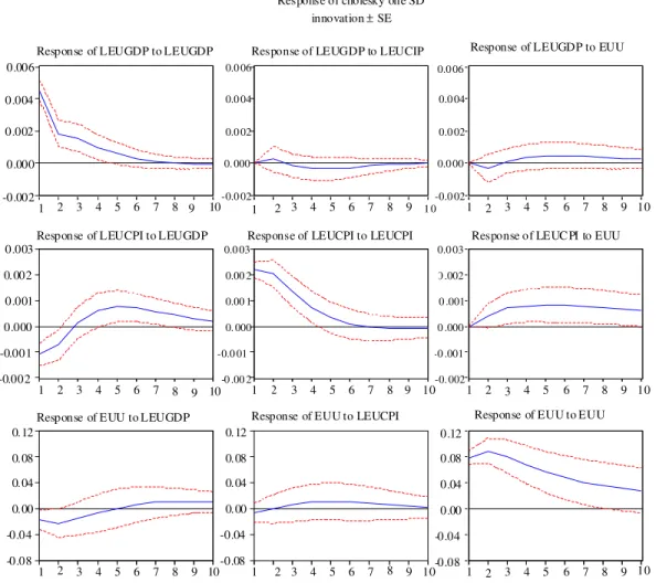
are affecting positively Y*; no policy instrument has any effect on P*; and i*OND and g* have a negative effect on unemployment. Figure 1 and 2 show the impulse responses after a shock on the innovation variable and its transmission to all the other endogenous (objective) variables through the dynamic (lag) structure of the VAR (Table 8). The above results support our hypothesis that the European integration has caused a very high cost to Greece, which exceeds the benefits.
Some socio-political implications of macroeconomic shocks and public policy ineffectiveness: Countries are different in Europe; for this reason their independence and sovereignty is necessary (even
though that the pressure they encounter from the globalists is tremendous). Each one nation faces its own idiosyncratic shocks; then, self-sufficiency is necessary, also independent public policies are needed to stabilize the domestic economy and improve the domestic welfare, which depends on the socio-philosophical conditions and value system of the country and not on some value neutral economic and financial indicators imposed by the EMU. We need a continuous improvement in our societies for the benefits of all the citizens, who have dual needs (physical and spiritual).
-0.004 0.000 0.004 0.008
1 2 3 4 5 6 7 8 9 10 Re sponse of LGRGDP to LGRGDP
-0. 004 0. 000 0 .004 0 .008
1 2 3 4 5 6 7 8 9 10
-0.0 04 0.0 00 0.0 04 0 .008
1 2 3 4 5 6 7 8 9 10
-0.004 0.000 0.004 0.008
1 2 3 4 5 6 7 8 9 10 -0 .004
0.0 00 0 .004 0 .008
1 2 3 4 5 6 7 8 9 10
-0.0 04 0 .000 0. 004 0. 008
1 2 3 4 5 6 7 8 9 10
-0.2 -0.1 0.0 0.1 0.2 0.3 0.4
1 2 3 4 5 6 7 8 9 10
-0.2 -0.1
0.0 0.1 0.2 0.3 0.4
1 2 3 4 5 6 7 8 9 10
-0.2 -0.1 0.0 0.1 0.2 0.3 0.4
1 2 3 4 5 6 7 8 9 10
Response of LGRGDP to LGRCOIUA Response of LGRGDP to GRU
Response of LGRCPI UA to LGRGDP Response of LGRC PIUA to LGRCPIUA Response of LGRC PI UA to GRU
Response of GRU to LGRGDP Re sponse of GR U to LGRCPIUA Response of GRU to GRU Response to cholesky one SD
innova tions ± 2 SE
Fig. 1: The impulse responses in Greece. Note: LGRGDP = ln of Greece’s GDP, LGRPIUA = ln of Greece’s price index and GRU = Greece’s unemployment rate. Source: Table 8
but not in such massive amounts as it is required with the low return on the European rates. In the context of imperfect capital mobility, the government can attain the goals of internal balance (full employment) and external balance (balanced payments) through the use of a fiscal and monetary policy mix. But, here, the objective of the country cannot be satisfied because the Maastricht criteria put restrictions on the country’s variables and domestic public policies are ineffective. Our concern is the determination of output (and employment), prices (inflation), interest rates, current account balance and other variables in these two economies (Greece and EMU) operating under a common flexible exchange rate. We are particularly interested in the problem of EMU suffering from unemployment and of Greece from high interest rates and current account deficits, national debt, unemployment and lost of her sovereignty. Their national, business and households debts are very high in
both entities, which have disastrous personal and social effects currently, due to the financial crisis and the recession and might have catastrophic consequences effects in the future on both economies.
In a world of managed (dirty) floating exchange rates, the Central Banks intervene from time to time in foreign exchange markets, which will affect the international reserve holdings of central banks (Fed, Bank of England, Bank of Japan, Swiss Central Bank and ECB). Many times, they do not allow the exchange rate to adjust to guarantee external payments balance. Then, the economy’s international transactions carried out and recorded by the Current Account (CA) and Capital Account (KA) are not balanced to zero, but an official reserve settlements account (OS) requires to make the Balance of Payments (BP) zero:
1 2 3 4 5 6 7 8 9 10 1 2 3 4 5 6 7 8 9 10 1 2 3 4 5 6 7 8 9 10 -0.002
0.000 0.002 0.004 0.006
1 2 3 4 5 6 7 8 9 10 Response of LEUGDP to LEUGDP
-0.0 02 0. 000 0.0 02 0.0 04 0.0 06
1 2 3 4 5 6 7 8 9 1 0
-0.0 02 0.0 00 0.0 02 0.0 04 0.0 06
1 2 3 4 5 6 7 8 9 10
-0.002 -0.001 0.000 0.001 0.002 0.003
1 2 3 4 5 6 7 8 9 10
1 2 3 4 5 6 7 8 9 10 1 2 3 4 5 6 7 8 9 10
-0.08 -0.04 0.00 0.04 0.08 0.12
Response of LEUGDP to LEUCIP Response of LEUGDP to EUU
-0 .00 2 -0.0 01
0. 000 0.00 1 0.00 2 0.0 03 Response of LEUCPI to LEUGDP
-0. 002 -0 .001 0 .000 0 .001 0 .002 0.0 03
Response of LEUCPI to LEUCPI Response of LEUC PI to EUU
-0.08 -0.04 0.00 0.04 0.08 0.12
-0.08 -0.04 0.00 0.04 0.08 0.12
Response of EUU to LEUGDP Response of EUU to LEUCPI Response of EUU to EUU Response of cholesky one SD
innovation ± SE
Fig. 2: The impulse responses in the EMU. Note: LEUGDP = ln of EMU GDP, LEUCPI = ln of Euro-zone consumer price index and EUU = Euro-zone unemployment rate. Source: Table 8
The central banks’ holdings of international reserves are influenced by the international transactions of domestic and foreign residents. At a given level of the exchange rate (E) and in the absence of any disturbances affecting autonomous spending, Eq. 6 and 2 provide us with the combinations of domestic prices (p) and incomes (Y ) that create equilibrium in the aggregate economies (AD = AS). These are the AD and AS curves. A rise in the nominal money supply increases real money balances, at a given level of the price of domestic goods. As domestic interest rates decline, investment and aggregate demand for domestic goods increase, at a given level of price and shifts the AD schedule to the right. This increase in AD will affect the prices gradually. As the price of domestic goods increases, employment will also tend to rise over the short run. The result is an increase in output. As prices rise, employment increases, because real wage is declining.
Changes in the nominal money supply induce shifts of the AD curve. An open market purchase will clearly increase the money supply and at a given price level, the resulting increase in real money balances would then place downward pressure on domestic interest rates, inducing capital to flow out of the economy and depreciating domestic currency. Unfortunately, Greece has lost her policy tool and the entire economy will suffer, until she will go back to drachma. Then, the consequence would be an expenditure switch out of foreign and into domestic goods, with a resulting increase in spending on domestic goods. This corresponds to a shift of the AD curve to the right. An expansion of demand for domestic goods and services has become necessary for small EMU economies, which have high unemployment and foreign trade deficits.
real labor costs associated with this disturbance. With nominal wage rates rigid over the short-run, the inflationary spur associated with the monetary expansion will reduce real wage rates. These reduced real labor costs and the consequent stimulus to domestic production have, as a counter part, a greater competitiveness of domestic goods in international markets, which is reflected in an increased real exchange rate. Of course, the labor cost has declined in Greece, due to illegal migration, pressure from the ECOFIN and the current deep recession.
In conclusion, the short-run expansionary impact of the monetary disturbance is closely linked to the decline of real wages, which spearheads an increase in net exports. Then, an expansion of the money supply will tend to shift the aggregate demand curve upward. By increasing the money supply, policy makers could, in principle, move the economy to full employment. It speeds it up by igniting inflation and therefore reducing real wages in the short-run. A domestic monetary expansion leading to increases in nominal and real exchange rates (currency depreciation) raises AD by improving the trade balance. But, members of EMU cannot have these benefits. At the same time, this policy implies that the foreign countries whose currencies appreciate both in nominal and real terms will face deteriorating net exports and a contraction of AD. Expansionary domestic monetary policy raises domestic real income-albeit, if temporarily at the expense of a reduction in real income abroad. Then, international policy conflicts arise from currency-depreciating policies under flexible exchange rates. These public policies effects have been lost for the EMU members, because of their common currency (euro) since January 1, 2002. On the other hand, the US has benefited from the depreciated dollar the last 6 years.
The aggregate demand curve is derived on the basis of a given level of the money supply, price level, the exchange rate, the TOT, aggregate spending, foreign income and fiscal policy parameters. Changes in any of these variables will tend to shift the AD curve. Also, any expansionary fiscal (monetary) policy has a positive multiplier effect on the AD for domestic goods, at any given level of prices shifting the AD curve to the right. Further, any increase in foreign income has a positive effect on our AD, depending on the foreign income elasticity of their demand for imports. Finally, a country must produce all goods and services that its citizens need, otherwise it has to become a net importer and a continuing borrower from abroad. Public policies are facing restrictions from ECB and ECOFIN and their effects on AD are very limited.
There is no question that public policies are playing a major role in our economies and affect the real macro-variables and our lives. Now, due to recession and low personal income, AD is very weak. On the other side, we have the production of a nation, the Aggregate Supply (AS). The interaction of AS and AD determines the equilibrium level of output (real income) and prices in the economy. The aggregate supply is derived on the basis of given wages, TOT, price of oil, exchange rate and unemployment rate. As the price of domestic goods increases, employment will also tend to rise over the short run. The result is an increase in output. This positive relationship between changes in prices and quantity supplied of domestic goods in the short run is the short run AS curve of domestic goods. As prices rise, employment increases because real wage is declining, then the output increases.