Rebalancing
Frequency and the
Welfare Cost of
Inflation
André C. Silva
Working Paper
# 587
Rebalancing Frequency and the Welfare Cost of In
fl
ation
André C. Silva
∗Nova School of Business and Economics
Abstract
Cash-in-advance models usually require agents to reallocate money and bonds infixed periods, every month or quarter, for example. I show thatfixed periods underestimate the welfare cost of inflation. I use a model in which agents choose how often they exchange bonds for money. In the benchmark specification, the welfare cost of ten percent instead of zero inflation increases from 0.1 percent of income withfixed periods to one percent with optimal pe-riods. The results are robust to different preferences, to different compositions of income in bonds or money, and to the introduction of capital and labor.
JEL Codes: E3, E4, E5.
Keywords: portfolio rebalancing frequency, welfare cost of inflation, money demand, cash-in-advance models, market segmentation.
∗Nova School of Business and Economics, Universidade Nova de Lisboa, Campus de Campolide,
1. Introduction
I calculate the welfare cost of inflation in a cash-in-advance model in which agents
vary the trading periods of bonds for money, as in Baumol (1952) and Tobin (1956).
I show that endogenizing the trading periods increases the welfare cost of inflation.
When the timing of bond market trades is fixed, the elasticity of the demand for
money with respect to the interest rate is small and the welfare cost of inflation is
small. When the timing of bond market trades is endogenous, an increase in inflation
makes agents trade more frequently. The demand for money becomes sensitive to the
interest rate, thefit to the data improves, and the welfare cost of inflation increases. I
show that an increase in inflation from zero to ten percent per year leads to a welfare
cost of one percent of GDP when the timing of bond market trades is allowed to
respond to inflation. The welfare cost is zero when the timing is fixed. With U.S.
GDP in 2000, a welfare cost of one percent of GDP corresponds to100 billion dollars
per year; or 900 dollars given to every household every year forever (data on GDP
and on the number of households from the BEA and the U.S. Census Bureau).
To study whether fixed periods affect results, I compare the welfare cost from
two cash-in-advance models: one in which agents choose how often to trade bonds
for money and another one in which agents trade bonds for money in fixed
peri-ods. It is optimal for each agent to increase the trading frequency when inflation
increases. However, increasing the trading frequency affects equilibrium through a
market clearing condition. The increase in the trading frequency increases
trans-actions costs, which reduces welfare. Taking into account that agents change their
trading frequency substantially increases the welfare cost estimates. A similar effect
occurs with distortionary taxation. It is optimal for each agent to decrease labor when
the income tax increases. But the aggregate decrease in labor implies a decrease in
The results on the welfare cost are related to the ability of cash-in-advance models
to match data on interest rates and money. According to the data, an increase in
the interest rate makes the real demand for money decrease. With fixed periods,
the demand for money is approximately constant, it is inelastic with respect to the
interest rate. Without further frictions, the welfare cost is approximately equal to
the area under the demand for money above equilibrium money holdings. This area
increases with the elasticity of the demand for money. An inelastic demand for money,
therefore, implies zero welfare cost of inflation. Optimal periods imply more elasticity,
a better match of interest rates and money, and a higher welfare cost of inflation.
Cash-in-advance models, in which agents buy goods with all balances from the
previous period, with a constraint such as 11 ≤0, imply money velocity equal to
one and so an inelastic demand for money by construction. Allowing cash and credit
goods or changing the trading sequence (trading bonds before or after trading goods)
implies variation in velocity. But Hodrick et al. (1991) show that the variation of
velocity is small.
Velocity varies more when agents hold money for many periods, with11++
≤ 0. In this case, different groups of agents trade bonds for money every
1 periods. This is the tradition of market segmentation initiated by Grossman
and Weiss (1983) and Rotemberg (1984). Alvarez et al. (2009) show that this type of
model matches the data on the short-run variation in velocity. However, as pointed
out by Romer (1986) and Grossman (1987), the models with fixed generate no
variation in long-run velocity. Even with large, the demand for money is inelastic.
Here, I allow to vary according to the interest rate. For realistic parameter
values, this change implies a long-run demand for money with−05 elasticity
(semi-elasticity of −125) and a better match with the data. As in the literature of market
segmentation, agents trade in different periods. The difference is that I let agents
compli-cates the problem, but it still allows the analytical characterization of the problem. I
obtain formulas for the demand for money and for the welfare cost of inflation, which
facilitates the analysis of the results.
A known result of market segmentation is that should be large to match data
on velocity (Edmond and Weill 2008). Alvarez et al. (2009), for example, require
intervals of 24to 36 months. This paper is not an exception. Ifind intervals of 6to
16months. (Smaller intervals because I use M1 instead of M2 as monetary aggregate.
I use M1 to make my results comparable to Lucas 2000, Lagos and Wright 2005, and
others.)
There are two potential problems with a large: (1) High intertemporal
substitu-tion facilitates the variasubstitu-tion of consumpsubstitu-tion within holding periods and might change
results. (2) Large trading intervals imply that agents accumulate interest in bonds
for long periods and, therefore, make large transfers of money. I show that neither
of the two problems is important. The welfare cost withfixed periods of ten percent
instead of zero inflation is always small. And optimal trading periods always yield a
welfare cost about one percentage point higher.
To study if other means to react to inflation could change results, beyond the
de-cision on consumption and rebalancing frequency, I make an extension of the model
for capital and labor. The results are robust. Ifind that the welfare costs in terms of
income of ten percent instead of zero inflation increase in parallel, about03
percent-age points in terms of income, for fixed and endogenous periods. The welfare cost
with endogenous periods is still one percentage point higher.
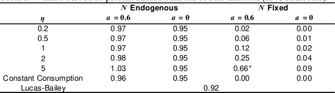
Table 1 shows the main message of the paper: the estimates of the welfare cost
increase from approximately zero to one percent with optimal periods. The table
shows the case with logarithmic utility and when agents receive zero or a fraction
of income in money, , promptly available for consumption. I consider zero or a
Thomas 2010, interpreted as the fraction of labor income in total income).
a = 0.6 a = 0 a = 0.6 a = 0
Logarithmic Utility 0.97 0.95 0.12 0.02
a: fraction of income received in money. Values from table 2 in section 4.
Table 1. Welfare cost of 10 percent inflation instead of zero inflation (in % of income)
Optimal Periods Fixed Periods
2. The Model
Agents manage money holdings by solving a Baumol (1952) and Tobin (1956)
problem of money as inventory: they have to use money to buy goods, only bonds
receive interest, and there is a cost to transfer the proceeds from bond sales to the
goods market. I use the term agents instead of households or consumers because
more than 62 percent of M1 in the U.S. is held by firms (Bover and Watson 2005).
The money holdings of consumers and firms in the economy are represented by the
money holdings of agents in the model. The model has elements of Jovanovic (1982),
Romer (1986), and Grossman (1987).
There is a continuum of agents with measure one. Each agent has a brokerage
account and a bank account, as in Alvarez et al. (2009). The brokerage account is
used to hold bonds and the bank account is used to hold money for goods purchases.
Time is continuous, ≥0. Let0denote money in the bank account at time zero and
0 denote bonds in the brokerage account at time zero. Index agents by= (0 0).
The agents pay a cost Γ in goods to transfer resources between the brokerage
account and the bank account. Γ represents a fixed cost of portfolio adjustment.
Let (), = 12 , denote the times of the transfers of agent . Let () denote
the price level. At (), agent pays (())Γ to make a transfer between the
brokerage account and the bank account. The agents choose the times of the transfers.
unit of labor. Let the transfer cost be given by Γ = , linear in income. With
this, the budget constraint of the agents and the demand for money will be linear in
income. The income elasticity of the demand for money will be equal to one, which
matches the evidence as stated in Lucas (2000) and others.
The agent is a composition of a shopper, a trader, and a worker, as in Lucas (1990).
The shopper uses money in the bank account to buy goods, the trader manages the
brokerage account, and the worker supplies one unit of labor to the firms. The firms
keep a fractionof the sales proceeds in money, transfer the remaining fraction1−
to their brokerage accounts, and convert this portion into bonds.
Thefirms pay() in money and(1−) () in bonds for the unit of labor
supplied. The firms make the payments in money with the money kept in the firm
and the bond payments with a transfer from the brokerage account of the firm to
the brokerage account of the agent. With the payments of the firm, the bank
ac-count of the agent is credited by () and the brokerage account is credited by
(1−)(). These credits can be used at the same date for the purchases of goods
and bonds.
Money holdings at timeof agentare denoted by( ). Money holdings just
af-ter a transfer are denoted by+(
() )and they are equal tolim→( ).
Analogously,−(() ) = lim→( )denotes money just before a
trans-fer. The net transfer from the brokerage account to the bank account is given by
+−−. If + −, the agent makes a negative net transfer, a transfer from
the bank account to the brokerage account, immediately converted into bonds. Money
holdings in the brokerage account are zero, as bonds receive interest and it is not
pos-sible to buy goods directly with money in the brokerage account. All money holdings
are in the bank account. To have + just after a transfer at
(), agent needs
to transfer +−−+(
goods to pay the transfer cost.1
The agents choose consumption ( ), money in the bank account ( ), and
the transfer times (), = 12 They make this decision at time zero given the
paths of the interest rate and of the price level. Let the price of a bond at time zero be
given by (), with (0) = 1. The nominal interest rate is () ≡ −log().
The maximization problem of agent is then given by
max
∞
X
=0
Z +1()
()
−(( )) (1)
subject to
∞
X
=1
(())£+(() ) + (())¤≤
∞
X
=1
(())−(() )+0(),
(2)
˙
( ) =− ()( ) +(), ≥0, 6=1() 2() , (3)
( ) ≥ 0, +1() ≥ (), given 0 ≥ 0, where 0 is the intertemporal
rate of discount and 0() ≡ 0 +R0∞() (1 −)() . To simplify the
ex-position, 0() ≡ 0, but there is not a transfer at = 0, unless 1() = 0. At =
1() 2() , constraint (3) is replaced by˙ (() )+=− (())+(() )+
(()), where ˙ (() )+ is the right derivative of ( ) with respect to
time at =() and+(() ) is consumption just after the transfer.
The utility function is (( )) = (1−)11−1, for = 16 , 0; and (( )) = log( ), for = 1. Preferences are a function of goods only, the transfer cost does
not enter the utility function. is the elasticity of intertemporal substitution.
The constraint (2) states that the present value of money transfers and transfer
1There are many other ways of defining theflows of money and bonds in the model. For example,
the agent at could sell+−−+Γbonds and payΓto the bank that holds the brokerage
account. The bank would then buy goods fromfirms and authorize the transfer of+
−−to the
fees is equal to the present value of deposits in the brokerage account, including
initial bond holdings. Constraint (3) states that money holdings decrease with goods
purchases and increase with money receipts. This constraint shows the transactions
role of money: agents need money to buy goods. As bonds receive interest and money
does not, the agents transfer the exact amount of money to consume until the next
transfer. That is, the agents adjust +(
), , and +1 to obtain −(+1) = 0,
≥ 1. We can still have −(1) 0 as 0 is given rather than being a choice.
Using (3), as −(
+1) = 0 for ≥1, money just after the transfer at is
+(
() ) = Z +1
()( )− Z +1
() , = 12 (4)
The government collects seigniorage and redistributes it to agents as initial bonds.
The government budget constraint is
0 =
R∞
0 () ()
˙
()
(), where
0 is the
ag-gregate quantity of bonds and() is the aggregate money supply. The government
controls the aggregate money supply at each time.
The market clearing conditions for money and bonds are() =R ( )()
and
0 =
R
0()(), where is a given distribution of . The market clearing
condition for goods takes into account the goods used to pay the transfer cost. Let
( ) ≡ { : () ∈ [ +]} represent the set of agents that make a transfer
during [ +]. The number of goods used on average during [ +] to pay the
transfer cost is then given byR()1
Γ(). Taking the limit to obtain the number
of goods used at time yields that the market clearing condition for goods is given
byR ( )() + lim→0
R ()
1
Γ() =.
An equilibrium is defined as prices (),(), allocations( ),( ), transfer
times (), = 12 , and a distribution of agents such that (i)( ),( ),
and() solve the maximization problem (1)-(3) given () and() for all ≥0
market clearing conditions for money, bonds, and goods hold.
The advantage of this version of the Baumol-Tobin model is being a standard
cash-in-advance model with the additional decision on the time to trade bonds for money.
The model has intertemporal discounting, infinitely-lived agents, and optimization
with consumption smoothing. These assumptions are common in cash-in-advance
models but have not been considered simultaneously in a Baumol-Tobin model.
(Jo-vanovic 1982, for example, assumes constant consumption; Romer 1986 assumes
over-lapping generations and zero intertemporal discounting. Other related models are in
Heathcote 1998, Chiu 2007, and Rodriguez-Mendizabal 2006.) By comparing the
cases with fixed and optimal periods, we can use the model to evaluate how much
fixed periods change estimations of the welfare cost of inflation.
3. The Demand for Money
Focus on an equilibrium in the steady state, an equilibrium such that the nominal
interest rate is constant at and inflation is constant at. The transfer cost implies
that it is optimal to rebalance the portfolio of bonds and money infrequently.
There-fore, I look for an equilibrium in which agents follow ( ) policies on consumption
and money. Moreover, I look for an equilibrium in which all agents have the same
consumption pattern within holding periods and choose the same interval between
transfers .
The demand for money depends on and on the consumption pattern followed by
the agents. The consumption pattern, in turn, depends on the distribution of agents as
the aggregation of individual consumptions must satisfy the market clearing condition
for goods. Therefore, we have to obtain the distribution of agents, the consumption
pattern, and to characterize the equilibrium and, especially, the demand for money.
Let ∈ [0 ) denote the position of an agent in a holding period in a steady
on. Consider the distribution of agents along[0 )compatible with the steady state
(with the properties of the steady state, we can then obtain the values of0 and0
of each agent such that the economy starts in the steady state). As the market
clearing condition requires constant aggregate consumption and the agents follow the
same consumption pattern, the number of agents that makes a transfer at each time
in the steady state must be constant. Therefore, the distribution of agents along
[0 )compatible with the steady state is uniform, with density1. It is possible to
have other distribution of agents if agents have different consumption patterns within
holding periods. To study the steady state, however, it is natural to have agents with
the same consumption pattern and consequently a uniform distribution.2
Consider now the pattern of consumption of each agent. Thefirst order conditions
of the maximization problem of the agent with respect to consumption imply( ) =
−
[()()()], ∈ ( +1), = 12 , where () is the Lagrange multiplier of
(2). Write consumption within holding periods as ( ) = 0(−−)−(−),
taking the largest such that ∈[(), +1()), where0, common for all agents,
denotes consumption at the beginning of a holding period. As shown in the appendix,
aggregating ( )at time implies () =0(−−)1− −
.
Therefore, aggregate consumption grows at the rate (−−), for arbitrary
and . If increases, the growth rate of aggregate consumption increases, as in an
economy with a representative agent. In equilibrium, = +, as a constant
requires aggregate consumption to be constant in equilibrium. The real interest rate,
defined as −, is then constant and equal to .
As = + in the steady state, individual consumption follows the pattern
( ) = 0−(−), decreasing within holding periods. The agents start a holding
2A proof that the uniform distribution is the only distribution of agents compatible with a
period with consumption0 and consume −0 just before a new transfer. However,
aggregate consumption is constant. A constant aggregate consumption coexists with
decreasing individual consumption although individual consumption decreases faster
when the nominal interest rate increases. The same happens with money, each agent
has a decreasing money-income ratio, equal to zero at the end of holding periods, but
the aggregate money-income ratio is constant over time.3
Increasing orincreases consumption in the beginning of holding periods.
Even-tually, it makes agents try to increase consumption by setting ( ) in the
end of holding periods. As ( ) = R+1
() [( )−], ∈ ( +1),
this would imply ( )0. The constraint ( )≥0 rules out this possibility.
However, instead of imposing this constraint, it is simpler to solve the model by
as-suming that ( )≥ 0holds, substituting the expression of +(
() ) in (2),
and then checking if ( ) ≥ 0 holds. To guarantee that ( ) ≥ 0, I check if
( )≥. An interesting property of the model is that ( ) always holds
for the relevant range of and. That is, forbetween zero andfive andfrom zero
to sixteen percent per year (I discuss the data in more detail later). This property
facilitates the characterization of the demand for money and of the welfare cost.
The value of 0 is obtained with the market clearing condition for goods. In
the steady state, it implies 1 R00− + 1 = . Therefore, 0( ) =
¡
1− ¢ ³1−−
´−1
. The consumption-income ratio, ˆ( ) =( ), is then
ˆ
( ) = ˆ0( )−(−), independent of , where ˆ0( ) = 0( ) is the
consumption-income ratio at the beginning of a holding period.
We obtain with thefirst order conditions forand for consumption, as described
3Caplin and Leahy (2010) discuss other models with ( ) policies with differences between
in the appendix. The optimal interval between transfers is the positive root of
ˆ
0( )
∙
1−−(−1) (−1) −
1−−[+(−1)]
[+(−1)] ¸
=+
∙
−1
−
(−) −1
(−) ¸
, for 6= 1, and (5)
ˆ
0( )
∙
1− 1−−
¸
=+
∙
−1
−
(−) −1
(−) ¸
, for= 1, (6)
where ˆ0( ) =¡1− ¢ ³1− −
´−1
.
To analyze these equations, write (5) as = where ≡ and is defined
with the remaining terms (the reasoning is the same with equation 6). is the
marginal loss of increasing and is the marginal benefit of increasing, both in
real terms. is the marginal benefit because the agent postpones the payment of
the transfer cost when increases. This term appears in the first order conditions
as ()() [()−()]. So, the benefit of postponing the payment depends
on the difference between the nominal interest rate and inflation at . In the steady
state, ()−() =.
The term increases when increases, as the money transferred at loses value
for inflation from to +1. When is large, the losses are large as any remaining
balance from the transfer at values little at a time close to +1. In this case,
. When is small, the losses are small, which implies . The optimal
equalizes marginal benefits with marginal losses, setting =.
An increase in or in makes increase. The intuition for is that agents
can decrease the losses by making the consumption profile steeper during holding
periods. The agents then loose less for inflation because they leave little of the money
transferred at for the end of holding periods. In the same way, decreases the
promptly used in the goods markets. Therefore, an increase inor inwith constant
makes . To reestablish the equilibrium, increases.
Turn now to and , the classical factors that influence the holding period. If
increases, the losses during( +1) increase. To reestablish the equality=,
the agents decrease by decreasing the holding period. If increases, the benefit
of postponing the payment of the transfer cost increases, making . It is then
optimal to increase . Therefore, decreases with the nominal interest rate and
increases with the transfer cost, 0 and 0. (The proofs of the
effects of the parameters on are in Silva 2011.)
We can use the expressions (5) and (6) if ˆ( ) ≥ . As consumption decreases
within , it is sufficient to check whether ˆ0− . With = 16 percent per
year, = 5, and = 06, for example, we have ˆ0− = 071 06, and so we can
use the expressions above.
A second-order Taylor expansion around zero of the exponential terms in (6), with
= 0, implies ≈ q2, the square-root formula for the interval between transfers.
The approximation does not hold with 0. With = 06, ≈q024, 60percent
higher than the square root approximation.
The aggregate demand for money is 1
R
( )and so the money-income ratio
is () = (1) 1 R ( ). In the steady state, as () is constant, the rate
of inflation is equal to the growth rate of the stock of money. Therefore, () =
1
0 1
R
0(), using initial money holdings across agents. The values of 0()
are obtained byfinding the quantity of money necessary for agentto consume at the
steady-state rate during [0 ). The calculations and the values of 0() are shown
in the appendix. The values of 0() imply that−() = 0 in the steady state.4
4The last step to characterize the equilibrium is tofind the values of
0(). See Silva (2011) for
this last step. An agent with (0() 0())then chooses1=,+1− =, and consumes
at the steady state rate. An economy with (0() 0())distributed to agents ∈[0 ) is in
The money-income ratio is then
() = ˆ0( )−
()
+(−1)
∙
()−1
() −
(−)()−1 (−)()
¸
− 1 −
∙
(−)()−1 (−)() −1
¸
(7)
where () is given by (5) and (6), and ˆ0( ) = ¡1− ¢ ³1− −
´−1
. The
calculations to obtain()are in the appendix. ()does not depend on as (())
is linear in (or, as the income-elasticity of (()) is equal to one). The money-income
ratio depends on the interest rate, preference parameters, and . I write () to
emphasize the role of.
Figures 1 and 2 show data on the money-income ratio along with () given by
equation (7), with = 0, for fixed and optimal .5 The interest-elasticity of ()
is close to −12 for 02 ≤ ≤ 10, using (7) to calculate the elasticity numerically.6
With fixed , () is close to a straight line for ≤ 10. The model better fits the
data with optimal.
Calibration, data, and the behavior of the demand for money
There are four parameters to calibrate: , , and . I use M1 for the monetary
aggregate and the short-term commercial paper rate for the interest rate. The data
set is similar to the one used in Lucas (2000). M1 and the commercial paper rate
were also used by Dotsey and Ireland (1996), Lagos and Wright (2005), Craig and
Rocheteau (2008), among others. Data are annual from 1900 to 1997 (the last year in
which the commercial paper rate data are available from the same source). There is
a discussion about whether M1 is the best aggregate to study money demand (Teles
5As ≡
, having expressed in dollars and GDP expressed in dollars per year implies
that the units of are in years. The interpretation is that agents carry in money the equivalent of a fraction of the production of one year. For example, = 026, the average money-income ratio during the 20th century for the U.S., means that agents carry in money the equivalent of the production of about one quarter.
6The smallest interest-elasticity in modulus in this range of and is −049 for = 02 and
0 2 4 6 8 10 12 14 16 0.1
0.2 0.3 0.4 0.5
m
(y
e
a
rs
)
Nominal interest rate (% p.a.)
0 2 4 6 8 10 12 14 16 0
100 200 300 400 500
N
(
d
a
ys)
Nominal interest rate (% p.a.)
= 0.1, 1, 10
= 0.1, 1, 10 = 50
= 50
Fig. 1. Optimal : money-income ratio and interval between transfers when is
endogenous. U.S. annual data, 1900-1997, M1 and commercial paper rate. = 0. : elasticity of intertemporal substitution.
and Zhou 2005).7 The main reason that I use M1 and the commercial paper rate is
to facilitate comparison of the estimates obtained here with the estimates obtained
in the literature.
I set = 0 and = 06. With = 0, the economy behaves as a standard
cash-in-advance model: the agents work, the proceeds from work are separated from the
agents, and the agents use their income to buy goods only after reallocating bonds
and money. If the length of the time period is one quarter, agents can consume from
their sales only in one quarter. With 0, the agents can use some of their income to
buy goods before reallocating bonds and money. For= 06, I follow the calibration
7Another aspect is that some components of M1 pay a small but positive interest rate, which
0 2 4 6 8 10 12 14 16 0.1
0.2 0.3 0.4 0.5
m
(y
e
a
rs
)
Nominal interest rate (% p.a.)
0 2 4 6 8 10 12 14 16 0
100 200 300 400 500
N
(
d
a
ys)
Nominal interest rate (% p.a.)
=50
=100
=100
=50
=0.1,1,10
= 0.1, 1 = 10
Fig.2. Fixed: money-income ratio and interval between transfers when isfixed.
U.S. annual data, 1900-1997, M1 and commercial paper rate. = 0. : elasticity of intertemporal substitution.
in Alvarez et al. (2009), and Khan and Thomas (2010). Alvarez et al., and Khan and
Thomas interpret as the fraction of income received as wages.
I set the intertemporal discount to 3 percent per year. With this, going from
10 percent inflation to zero requires decreasing from 13 to 3 percent. I vary the
elasticity of intertemporal substitution from 01 to values as high as 100 (when
= 0). The estimates of are usually below 10 (Mehra and Prescott 1985, Bansal
and Yaron 2004, for example; Hansen and Singleton 1982, and Attanasio and Weber
1989 have larger estimates of ). I use the values of above 10 to show that setting
fixed periods only matches the data when is high. When is optimal, has little effect on the money-income ratio.
. A higher shifts the money-income ratio upward in the × diagram. I set
so that () matches the historical average on the money-income ratio and interest
rates (obtained with their geometric means). Lucas (2000) follows the same method
and, similarly, Alvarez et al. (2009), and Khan and Thomas (2010) use the historical
average of M2 velocity. The mean interest rate during 1900-1997 is 36 percent per
year and the mean money-income ratio is 026. The data, therefore, say that agents
hold on average about90days of income in money. These high historical values imply
= 179 for = 0 and = 1.8
Figure 1 shows the data and () for = 0 and = 01, 1, 10, and 50. It also
shows the interval between transfers for each and. The curves overlap, as has
little effect on and on the money-income ratio when is optimal. I include= 50
to compare the results with those with a fixed . Although the model simplifies
many features of an actual economy (for example, it abstracts from precautionary
motives for holding money, and aggregates households and firms in one agent), the
fit of the money-income ratio is surprisingly good.
The model is able to explain the high money-income ratio of the 1940s (the points
in the upper left corner; in 1946, = 081and = 048) and the low money-income
ratio of the 1980s (the points in the bottom right corner; in 1981, = 148 and
= 014). It explains the decrease in the money-income ratio from 1945 to 1981:
the money-income ratio decreased because the interest rate increased. The model does
not explain the high in the beginning of the century, with interest rates between
3 and 6 percent (just above the curve), and the low in the 1990s (just below the
curve), with approximately the same interest rates. But the model does describe the
general pattern of the data.
The curves infigure 1 overlap with the Baumol-Tobin money-income ratiop(2).
Lucas (2000) argues that the Baumol-Tobin money demand has a goodfit to the U.S.
data.
The money-income ratio decreases as the interest rate increases because the interval
between transfers is endogenous. () is approximately constant in if the interval
between transfers is fixed (Romer 1986 finds similar results with logarithmic utility).
What makes decrease is the ability of agents to change . That is, the ability to
change the frequency of portfolio rebalancing. If isfixed, is constant in .
Withfixed, could decrease because agents vary consumption within. This
effect is relevant only for high elasticities of substitution. As shown in figure 2, the
money-income ratio with fixed approximates the data only if is greater than50
( is fixed at the optimal value of when is equal to the historical mean of the
data, () with fixed and optimal coincide at the mean ). Letting agents
change is important to explain the empirical fact that the money-income ratio
decreases when the interest rate increases. Some early evidence about this behavior
is in Meltzer (1963) and Lucas (1988).
The values of implied by the model are large. With = 4 percent per year and
= 1, the interval between transfers is 181 days, which implies about two transfers
per year. These transfers are from high-yielding assets to cash. They are not ATM
withdrawals. Transfers convert bonds into money whereas ATM withdrawals convert
deposits into cash but do not change the quantity of money. There are two reasons
for the values of and . First, the average money-income ratio is high. Second,
households and firms hold a large quantity of money and make infrequent transfers.
First, the average money-income ratio, about one fourth of a year, is high in the
data. With per capita income of 35,000 dollars in 2000, = 026 implies that each
person in the U.S. holds about 9,000 dollars. Therefore, = 179and = 181 days
so that () matches the high historical money-income ratio. If we use more recent
data, = 01 in 2000, then decreases to 027 and to 70 days. I divide and
per transfer, the unit of is days per transfer. So = 027 means about one fourth
of a day. The cost per transfer is then 027×35,000365 = 26dollars. (Alternatively, dividing and by 260 working days implies = 019 working days per transfer,
= 52 working days and, again, 019×35000260 = 26 dollars.) However, we cannot use only the more recent data to estimate the demand for money and the
welfare cost of inflation. Moreover, to compare the results on the demand for money
and the welfare cost, we need to use the same data set as in previous studies.
Second, households and firms in fact trade infrequently and hold large quantities
of money. This behavior requires a large . Vissing-Jorgensen (2002), for example,
shows that a large fraction of households trade assets with higher yields less than
once a year. Christiano et al. (1996) show that households take a long time to adjust
their portfolios. Alvarez et al. (2009) state that only about half of the households
that held stocks bought or sold stocks in 1998-2001 (I later calibrate the model with
60 percent of income directly deposited into the bank account, as in Alvarez et al.).
Bates et al. (2009)find that the cash-assets ratio has been increasing strongly among
firms (as stated above, U.S. firms in 2000 held 62 percent of M1). These pieces of
evidence are puzzling given the financial innovations of the last decades. It is beyond
the objectives of this paper to study the individual behavior of households or firms.
For studies on household money holdings and firm cash holdings, see Alvarez and
Lippi (2009) and Bates et al. (2009).
The large value of is common in the literature (Edmond and Weill 2008). Alvarez
et al. (2009) set the transfer interval from 15 to 3 years (they calibrate directly
because is fixed in their model). Guerron-Quintana (2009), in a model with
port-folio adjustments, estimates that agents adjust their portport-folios every3to 6quarters.
The calibration in Khan and Thomas (2010) implies average transfer intervals from
12 to 24 years. Here, the calibration implies of about six months. A smaller
I close this section by studying the case with= 06, the same value used in Alvarez
et al. and Khan and Thomas.
When = 06, the agents receive sixty percent of their income in money. The
remainder is deposited in the brokerage account. As the agents receive a fraction of
their income in money without cost, they have less incentives to trade bonds for money
frequently. This effect increases and, keeping the same as with = 0, decreases
the financial cost. The money demand shifts downward. In order to reestablish the
match between and the data, the parameter has to increase. The increase in
is such that is approximately constant with = 0 or 06.
The money-income ratio changes little with equal to zero or large such as 60
percent when is endogenous. This can be seen infigure 3. The figure shows ()
with = 0 and 06, and with = 1 in the left panel and = 5 in the right panel.
When is optimal, the two curves for overlap with = 1. With = 5, we can
distinguish the two curves with different values of, but the difference is small. When
is fixed, = 06 makes decreasing in , but the difference between = 0 and
06is clear only with = 5. When is optimal, has almost no effect.
The reason for the small impact ofwith endogenous is that agents best manage
their money holdings by varying the transfer intervals. A higher is compensated by
a lower frequency of exchanges of bonds for money. That is, a higher. This shifts
downward without changing its elasticity. Once is recalibrated, the money-income
ratio returns to its previous position: increases from 179to466for = 1 when
increases to06. With = 4 percent, increases from 181 days to467 days. is
approximately constant when = 0 or 06, = 1 percent. In the next section, I
0 2 4 6 8 10 12 14 16 0.05 0.1 0.15 0.2 0.25 0.3 0.35 0.4 0.45 0.5 0.55
Nominal interest rate (% p.a.) Money-Income ratio, a=0 and a=0.6. =5
a=0, N Fixed
a=0.6, N Fixed
a=0, N Endogenous
a=0.6, N Endogenous
0 2 4 6 8 10 12 14 16
0.05 0.1 0.15 0.2 0.25 0.3 0.35 0.4 0.45 0.5 0.55 m (y e a rs )
Nominal interest rate (% p.a.) Money-Income ratio, a=0 and a=0.6. =1 (log utility)
a=0, N Fixed
a=0.6, N Fixed
a=0 and 0.6, N Endogenous
0 2 4 6 8 10 12 14 16
0.05 0.1 0.15 0.2 0.25 0.3 0.35 0.4 0.45 0.5 0.55
Nominal interest rate (% p.a.) Money-Income ratio, a=0 and a=0.6. =5
a=0, N Fixed
a=0.6, N Fixed
a=0, N Endogenous
a=0.6, N Endogenous
0 2 4 6 8 10 12 14 16
0.05 0.1 0.15 0.2 0.25 0.3 0.35 0.4 0.45 0.5 0.55 m (y e a rs )
Nominal interest rate (% p.a.) Money-Income ratio, a=0 and a=0.6. =1 (log utility)
a=0, N Fixed
a=0.6, N Fixed
a=0 and 0.6, N Endogenous
Fig. 3. Left: = 1, log utility. Right: = 5. A fraction 0 in money affects
the economy only with high and fixed. 0 as high as 06 changes little the money-income ratio when is endogenous.
4. The Welfare Cost of Inflation
Agents use part of their resources for financial services when 0. The optimal
monetary policy is to set = 0. The Friedman rule applies (Friedman 1969).
The income compensation () so that agents are indifferent between and ¯is
defined as [(1 +())] = (¯ ), where ( ) is the aggregate utility
from all agents with equal weight, ( ) = 1
1
R
0
[0(;)−]
1−1
1−1 . Therefore,
the income compensation is
1 +() = 0(¯)
0()
"µ
1−−(−1) (−1)
¶−1
1−−¯(−1) ¯
¯
(−1) ¯ # 1
1−1
, for 6= 1, and (8)
1 +() = 0(¯)
0() exp µ 2 − ¯ ¯ 2 
, for= 1.
¯
= 3). It shows the role of the fraction of income in money, and the role of fixed or
endogenous . As mentioned earlier, = 0 or 06 has a small effect on the
money-income ratio when is endogenous. In the same way, increasing from 0 to 06
slightly increases but changes little the welfare cost when is endogenous.
A fractionof60percent could greatly change the welfare cost because agents gain
access to a large part of their income earlier. Surprisingly, it has no effect. What
matters is the fraction of income devoted to financial transfers: the product between
the cost of one transfer as a fraction of income and the frequency of transfers,×1. With = 4 percent per year and log utility, = 1 percent (for = 0 or 06),
which means that agents devote one percent of their time to manage money holdings.
Workers in the U.S. worked about 1,900 hours per year on average from1950to1997
(OECD data). When= 4percent, therefore, the model estimates about22minutes
per week devoted tofinancial services.
η a = 0.6 a = 0 a = 0.6 a = 0
0.2 0.97 0.95 0.02 0.00
0.5 0.97 0.95 0.06 0.01
1 0.97 0.95 0.12 0.02
2 0.98 0.95 0.25 0.04
5 1.03 0.95 0.66* 0.09
Constant Consumption 0.96 0.95 0.00 0.00
Lucas-Bailey
Table 2. Welfare cost of 10 percent inflation instead of zero inflation (in % of income)
Constant consumption: η=0.001. Lucas-Bailey: area under the Baumol-Tobin money demand. Welfare cost: w(r) from r=13% p.a. to r=3% p.a. η: elasticity of intertemporal substitution.
N Endogenous N Fixed
0.92
*: for 9.5% inflation (c>=aY binds for 10% inflation, η=5, a=0.6, and N Fixed).
approximates the welfare cost of a positive interest rate. The cost of10percent
inflation instead of zero inflation can then be approximated by the difference between
()when = 13and3percent,=13−=3. With log utility, this difference
equals093 percent. The welfare cost of 10percent inflation using (8) for = 0 and
and the welfare cost can also be related by the method used by Bailey (1956),
calculating the area under the demand for money above equilibrium money holdings.
As stated in Lucas (2000), R0()−(). The model generates a demand for
money close to the Baumol-Tobin money demandp(2). In this case, the method
of Bailey yieldsp2, which is approximately when ≈p2. Lucas (2000)
uses the method of Bailey with a Baumol-Tobin money demand as a benchmark for
the welfare cost of inflation. The Lucas-Bailey measure p2 is smaller, but close
to(), as shown in table 2.
() decreases substantially when is fixed as it can be seen in table 2. With
= 0, the welfare cost is approximately zero. One way of understanding this result
is that the demand for money is approximately constant with fixed. As the area
under the demand for money above equilibrium money holdings approximates the
welfare cost, the welfare cost with fixed is close to zero.
The parameter increases () when is fixed because the demand for money
is more elastic. The elasticity of the demand for money increases with because a
higherallows agents to vary consumption more easily within holding periods. With
fixed, agents can decreaseonly by increasing the variation of consumption, which
is easier to do when increases (the effect on () is small when is endogenous
because the demand for money is already elastic in this case). The effect of is stronger than the effect of because = 06 implies a demand for money more negatively sloped, but this effect is important only ifis high: increases()from
zero to 01 percent with log utility and to07 percent with = 5. Even with = 5,
it is still lower than the welfare cost with endogenous. The relation of () with
the demand for money is used to explain the effects of the parameters. With the
exception of the Lucas-Bailey case, all values in table 2 were obtained from (8).9
9We have to check whether()≥ to use the expressions in (8). The constraint binds only
Why does an endogenous make the welfare cost increase? In principle, an
en-dogenous had to imply a smaller welfare cost, as agents choose to maximize
utility. What happens in the model is similar to the effects of an increase in a
dis-tortionary tax such as the income tax. With endogenous labor supply, it is optimal
for each agent to decrease the labor supply if there is an increase in the income tax
rate. In the new equilibrium, the decrease in labor reduces aggregate output (an
effect not considered by the agents when solving their maximization problems) and
reduces welfare by more than the gains from reducing labor supply.
Here, it is optimal for each agent to decrease when increases. The agents take
into account that they have to pay the adjustment cost more often and willingly do so.
However, they do not take into account that the equilibrium changes whenincreases.
The model also takes into account the higher variation of consumption within holding
periods, but the more relevant effect is the increase infinancial services. In particular,
total resources diverted from consumption are equal to 1
. With endogenous ,
the welfare cost increases because the model takes into account the increase in the
use offinancial services.
Another way of understanding this result is that each agent is better offby reducing
when increases, taking the real values of money and bonds as given. But the
new equilibrium implies a different price level 0 and different real values of money
and bonds. These equilibrium changes are not taken into account by the agents when
they solve their individual maximization problems. Figure 4 shows this mechanism.
The figure shows the utility of a particular agent, agent = 0, after solving the
maximization problem of the agent. The real values of 0() and0()have to be
such that 1() agents make transfers at each time. Therefore, each steady state
with a nominal interest rateimplies a different price level0and different real values
of 0 and0 for each agent.
In thefirst diagram of figure 4, the real values of 0 and0 are kept constant at
their values compatible with the historical mean of the interest rate, = 36percent
per year (it could be any value of ). As the interest rate increases, the utility
decreases whether or not the agent is able to change . Given the real values of 0
and 0, utility decreases less with endogenous, as the agent adapts to the higher
inflation by decreasing .10
However, the real values of0 and0 compatible with a steady state with= 36
percent are not compatible with a steady state equilibrium with 36 percent.
With a higher , the price level changes. So, the real values of 0 and 0 change.
Their new real values satisfy the increase in the frequency of transfers of all agents
and the new market clearing conditions. When we recalculate the utility with the
equilibrium real values of 0 and0, utility decreases faster with endogenous.
2 4 6 8 10 12 14 16
Equilibrium real M
0 and B0
U
til
it
y
Nominal interest rate (% p.a.) N Endogenous
N Fixed
2 4 6 8 10 12 14 16
Constant real M
0 and B0
U
til
ity
Nominal interest rate (% p.a.) N Fixed
N Endogenous
2 4 6 8 10 12 14 16
Equilibrium real M
0 and B0
U
til
it
y
Nominal interest rate (% p.a.) N Endogenous
N Fixed
2 4 6 8 10 12 14 16
Constant real M
0 and B0
U
til
ity
Nominal interest rate (% p.a.) N Fixed
N Endogenous
Fig. 4. Utility of a single agent. Left: real 0 and0 constant at their equilibrium
values under the mean nominal interest rate, = 36%. Right: real 0 and 0
compatible with the steady state equilibrium for each interest rate. The welfare cost with endogenous is higher when we consider the general equilibrium effects.
10To obtain the figures, I also increased inflation, using = −, in order to imply the same
For both fixed and endogenous, in addition to the transfer cost, the variation
of ( ) within holding periods decreases welfare. The effect of the variation of
consumption is small for both fixed and endogenous for the levels of inflation
considered here. The effect of the increase in financial services is more important.
However, when is high, the variation of consumption with fixed can be so high
that the welfare cost can be higher with fixed (the variation of consumption is
smaller with endogenous because agents can adjust to decrease the variation
of consumption). This only happens with very high interest rates. The welfare cost
with fixed is equal to the welfare cost with endogenous when = 261 percent
per year, and it is higher with fixed for beyond this point. With this nominal
interest rate, () = 786 percent of income.
I focus on moderate inflation in table 2. I do not concentrate on the welfare cost
of small positive interest rates instead of the Friedman rule or of very high inflation.
Mulligan and Sala-i-Martin (2000) argue that the demand for money changes for
low inflation because having or not having a bank account, that is, the extensive
margin, becomes more important than the rebalancing frequency. Ireland (2009)
argues that a semi-log money demand better matches the data for low inflation.
For high inflation, in addition to changes in the money demand, we would have to
consider other factors such as the loss of information caused by inflation (Harberger
1998). Studying moderate inflation emphasizes the effects of the frequency offinancial
transactions. For moderate inflation,()changes little with log-log, as we have here,
or semi-log money demands (Lucas 2000). Moreover, rates of inflation between zero
and ten percent per year are the most common rates of inflation in OECD countries.
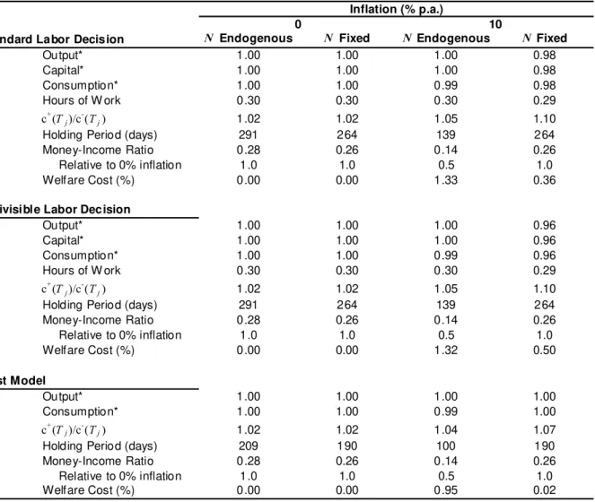
5. The Model with Capital and Labor
I now introduce the decisions on capital and labor. This extension allows us to
standard cash-in-advance model. Both with capital and endogenous labor supply. I
show that the calculations of the welfare costs are robust. The welfare cost increases
in parallel for fixed and endogenous periods. The welfare cost of 10percent instead
of zero inflation is still one percentage point higher with endogenous periods.
The expressions for the interval between transfers and for the money-income ratio
remain unchanged with capital and labor. As a result, the area under the demand
for money does not change. As the welfare cost increases, this extension puts in
evidence that the area under the demand for money is an approximation for the
welfare cost, but it does not take into account the full welfare cost of inflation (a
result also emphasized, for example, in Lagos and Wright 2005). With capital and
labor, the welfare cost of inflation increases about 03 percentage points for fixed
and endogenous. With endogenous, it increases to 133 percent of income.
Table 3 summarizes the effects of introducing capital and labor on the welfare cost of
inflation.
N Endogenous N Fixed Difference
Standard Labor Decision 1.33 0.36 0.97
Indivisible Labor Decision 1.32 0.50 0.83
No Capital or Labor (First Model) 0.95 0.02 0.93
Table 3. Welfare cost of 10% p.a. inflation instead of zero inflation (in % of income). The effect of introducing capital and labor.
Welfare cost: w(r) from r=13% p.a. to r=3% p.a . N Fixed: optimal choice of N under r=3.64% p.a., the geometric average of r over the period.
I use a standard cash-in-advance model with capital and labor, the difference is
the decision on the size of the holding periods. The model is similar to the models in
Cooley and Hansen (1989) and Cooley (1995).
Production is given by () = 0()()1−, where () and () are
ag-gregate capital and hours of work at time and 0 1. Capital depreciates at
the rate . Individual capital and hours of work are given by ( ) and ( ),
the real interest rate on capital () are given by () = (1−)
0
h ()
()
i
and
() =
0
h ()
()
i−(1−)
.
The government offers bonds that pay a nominal interest rate (). To avoid
the opportunity of arbitrage between government bonds and capital, we must have
()−() =()−. If this condition is violated, agents would arbitrarily increase
the quantity of bonds or capital in their portfolios.
Preferences now take into account consumption and hours of work. I consider the
logarithmic preferences ( ) = log+log (1−), 0, and the preferences for
indivisible labor( ) = log−, 0. I focus the exposition on the logarithmic
preferences, with standard labor decision. Both preferences are derived from( ) = [(1−)]1−1
1−1 with = 1 and are compatible with a balanced growth path (King et al.
1988). The preferences for indivisible labor were considered by Cooley and Hansen
(1989). They are obtained with= 1 and the additional assumption that agents can
only work zero or a certain positive number of hours (Hansen 1985).
The separability of consumption and hours worked obtained with = 1 implies
that, in the steady state, hours worked within holding periods are constant. Having
constant hours worked simplifies the analysis and facilitates the comparison of the
welfare cost of inflation with fixed or endogenous trading frequency. Having = 1
also facilitates the comparison with other estimates for the welfare cost of inflation
obtained in the literature.11
Agents make their decisions at = 0, given prices and their initial holdings of
11It is possible to obtain analytical formulas with 6= 1. However, the variation of hours worked
money0, bonds 0, and capital0. The maximization problem is
max
∞
X
=0
Z +1()
()
−[log( ) +log (1−( ))] (9)
subject to
∞
X
=1
(()) £
+(() ) + () () ¤
≤
∞
X
=1
(())−() +0(),
(10)
where +(
() ) =R(+1)() ()( ),˙ ( ) =− ()( ), and
0() =0 +00+
Z ∞
0
() ()()( ). (11)
With indivisible labor, the utility function changes to log( ) −( ). The
problem is written for the case with = 0, which simplifies the characterization of
the equilibrium. The purchase of capital and the income from capital appear in the
term 00 in the present value budget constraint. At (), agent sells bonds and
capital to start the holding period with +(() ) in money to be used in the
goods market. During a holding period[ +1), real holdings of bonds and capital
grow at the rates ()−() and()−. As ()−() =()−, the agents
are indifferent to the evolution of the two assets.12
The transfer cost Γ is given by (). If agents took () in Γ= () as their
own income, they would decrease labor and capital discontinuously at time to pay
12To obtain the present value budget constraint (10) use the constraint +(
) ++() +
()+() +()Γ=−() +−() +()−(),= 12 , where+,−,+, and
− are the quantities of bonds and capital just after and just before the transfer, and the fact that bonds and capital follow˙ () =()() +()()()and˙() =¡()−¢during holding
periods (as()−() =()−, it does not matter if labor income is invested in bonds, as the
equation for˙ implies). Substituting recursively and using the conditionslim→+∞()+() =
0andlim→+∞()()+() = 0imply (10). In a different context, Ljungqvist and Sargent
a smaller transfer cost. To rule out this possibility, each agent takes aggregate output
() as given, as the individual participation in aggregate output is small. As a
result, the transfer costΓ= () is also taken as given.
The market clearing conditions for money and bonds are the same as before. The
market clearing condition for goods now includes aggregate investment,˙ ()+().
Given a distribution of agents , the market clearing condition for capital and hours
of work are() =R ( )()and () =R ( )().
Solving the model with capital and labor
As in the case without capital and labor, focus on the equilibrium in the steady
state. In particular, the nominal interest rate is constant and the inflation rate is
constant. Now, moreover, the aggregate quantities of capital and labor are constant.
The first order conditions for consumption imply ( ) =0(−−)()−(+)(−
()), ∈(
+1),∈[0 ). This expression implies that aggregate consumption
is () =0(−−)1− −
. Therefore, the same relation holds between the nominal
interest rate and inflation to imply constant aggregate consumption, =+. The
non-arbitrage condition then implies =+.
With =+ and the expressions ofand from the maximization problem of
thefirms, the capital-hours ratio and the capital-output ratio are =
³ 0
+ ´ 1
1−
and
=
+. As ˙ = 0 in the steady state, the investment-output ratio in the steady
state is given by =
+.
The market clearing condition for goods implies++1 =. Therefore,
0() =
µ
1− 1
− +
¶ µ
1−−
¶−1
0
µ
(). (12)
Dividing by = 01−, we obtain the expression for the consumption-income
ratio just after a transfer,ˆ0() =
³
1− 1
− +
´ ³
1−−
´−1
, which is, apart from
As the expressions for and for the money-income ratio in (5)-(6), and (7) depend
only on ˆ0, the value of and the demand for money have the same expressions in
this economy with capital and labor.
Therefore, the fact that agents can now react to the change in inflation with changes
in capital and labor does not change the demand for money. In particular, this
extension shows that the area under the demand for money works as an approximation
for the welfare cost of inflation, but it does not account for the whole cost. Because
the demand for money is the same, the area under it from= 3 to = 13 percent is
also the same. However, the welfare cost of inflation increases for both fixed and
endogenous.
The first order conditions for( ) imply 1−( ) = 0, with = 010. As
is constant, ( ) =is constant over time. With the expression of , we obtain
the equilibrium value of the hours of work,
() = (1−) (1−) +ˆ0()
, (13)
where ˆ0() is the consumption-income ratio. (The preferences for indivisible labor
yield () = (1ˆ−)
0() following similar steps. The expressions for ˆ0(), (), (),
and()remain unchanged with indivisible labor.) Given that is constant across
time and across agents, aggregate hours of work are given by = 1 R0( )=
. With this, we have obtained all equilibrium variables to calculate the welfare cost
of inflation in this new economy.
The welfare cost of inflation is defined in the same way as in Section 4: as the
income compensation()to leave agents indifferent between an economy with ¯
and an economy with ¯, [((1 +()) ()) ()] = [(¯ (¯)) (¯)].