www.atmos-chem-phys.net/10/1/2010/
© Author(s) 2010. This work is distributed under the Creative Commons Attribution 3.0 License.
Chemistry
and Physics
Technical Note: Time-dependent limb-darkening calibration for
solar occultation instruments
S. P. Burton1,*, L. W. Thomason2, and J. M. Zawodny2 1SAIC, Hampton, Virginia, USA
2NASA Langley Research Center, Hampton, Virginia, USA
*now at: Science Systems and Applications, Inc., Hampton, Virginia, USA
Received: 4 June 2009 – Published in Atmos. Chem. Phys. Discuss.: 28 September 2009 Revised: 25 November 2009 – Accepted: 8 December 2009 – Published: 4 January 2010
Abstract.Solar occultation has proven to be a reliable tech-nique for the measurement of atmospheric constituents in the stratosphere. NASA’s Stratospheric Aerosol and Gas Ex-periments (SAGE, SAGE II, and SAGE III) together have provided over 25 years of quality solar occultation data, a data record which has been an important resource for the sci-entific exploration of atmospheric composition and climate change. Herein, we describe an improvement to the process-ing of SAGE data that corrects for a previously uncorrected short-term time-dependence in the calibration function. The variability relates to the apparent rotation of the scanning track with respect to the face of the sun due to the motion of the satellite. Correcting for this effect results in a decrease in the measurement noise in the Level 1 line-of-sight opti-cal depth measurements of approximately 40% in the middle and upper stratospheric SAGE II and III observations where it has been applied. The technique is potentially useful for any scanning solar occultation instrument and suggests fur-ther improvement for future occultation measurements if a full disk imaging system can be included.
1 Introduction
The Stratospheric Aerosol and Gas Experiment series of instruments, which includes SAGE (1979–1981), SAGE II (1984–2005), and SAGE III (2002–2006), employed the so-lar occultation technique to provide measurements of the pro-file of atmospheric constituents including ozone number den-sity and aerosol extinction coefficient. The data sets have been used in a broad range of applications, including climate
Correspondence to:S. Burton ([email protected])
change (Hansen et al., 1997), the climate impact of volcanoes (McCormick et al., 1995; Stenchikov et al., 1998), ozone trends (Solomon et al., 1997, 1998; Randel and Wu, 2007), and aerosol variability and trends (Thomason et al., 1998; SPARC, 2006).
The long lifetime of the instrument has permitted an evolv-ing understandevolv-ing of retrieval methods that has led to sub-stantial improvements of key data products like ozone rel-ative to early versions of the data sets (e.g. Cunnold et al., 1996; Steinbrecht, 2006; Terao and Logan, 2007). Herein, we describe an effort to further enhance the quality of SAGE data products by recognizing and reducing a previously un-corrected source of noise, namely the apparent rotation of the scan track across the face of the sun during the course of a measurement event. The rotation impacts the normalization process which is essential in the inference of the vertical de-pendence of transmission. In the frame of reference fixed to the satellite, the sun appears to rotate slightly as it rises or sets, while the scanning continues to be vertical (in the satellite frame) throughout the observation. This implies a mismatch between the limb darkening function in effect dur-ing the calibration phase and the atmospheric measurement phase of each observation event. The self-calibration of solar occultation data and the assumption of constant limb darken-ing will be described in more detail in the next two subsec-tions.
2 S. P. Burton et al.: Time-dependent limb-darkening calibration is easily applicable, amounts to approximately 40%. The
technique outlined here is potentially valuable to any solar occultation measurement that scans across the sun, not just the SAGE experiments. Furthermore, it suggests that a full-disk imaging camera on future solar occultation instruments would be highly useful, for it would allow precise calibra-tion with the appropriate limb darkening funccalibra-tion regardless of the rotation of the instrument relative to the Sun.
1.1 SAGE measurement technique
The SAGE II mission was terminated in August 2005, after more than 21 years of solar occultation measurements. The SAGE II data set consists of aerosol extinction measurements at four wavelengths, 1020 nm, 525 nm, 452 nm, and 386 nm; ozone and NO2number density; and water vapor mixing ra-tio. SAGE II was preceded by the original SAGE (now of-ten referred to as SAGE I), which provided ozone, NO2and aerosol extinction at 1000 nm and 450 nm. The SAGE III instrument (2002–2006) added to the suite of data products with temperature and pressure measurements, an expanded set of nine wavelengths for aerosol extinction profiles, and nighttime lunar occultation profiles of ozone, NO2, NO3, and OClO. Descriptions of instrument specifications are given by Mauldin et al. (1985) and SAGE III ATBD (2002).
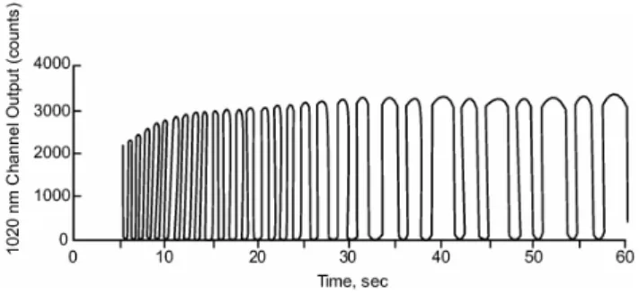
The three SAGE instruments made measurements using solar occultation, recording the attenuation of sunlight at multiple wavelengths through the Earth’s atmospheric limb during each satellite-observed sunrise and sunset. Solar occultation measurements are insensitive to calibration, in that transmittance measurements are formed by normaliz-ing the observations through the atmospheric limb by ob-servations during the same event along paths that do not intersect the atmosphere. Multiple transmittance measure-ments are obtained at each altitude by repeatedly scanning across the face of the sun as it rises or sets (Chu et al., 1989; SAGE III ATDB, 2002). Figure 1 illustrates an example of the SAGE data stream as a function of time for a sunrise event. In Level 1 processing, the measurements are com-bined to form a mean profile of transmission versus altitude at each wavelength, plus an uncertainty estimate, which is the input for Level 2 processing, where the contributions by various atmospheric constituents are separated and the slant path measurements are inverted into vertical profiles (Chu et al., 1989; SPARC, 2006; SAGE III ATDB, 2002). The uncer-tainty in the transmission data primarily consists of altitude registration errors for individual data points and normaliza-tion mismatch errors in registering the corresponding posi-tion of in-atmosphere data in the exoatmospheric scans. For SAGE II, electronic noise is generally well below the count level and not readily measurable.
As already mentioned, multiple transmittance measuments are obtained at each altitude as the instrument re-peatedly scans the sun. There are generally several mea-surements of transmission within each small altitude region,
Fig. 1. The time history of sunrise SAGE event at a single wave-length (1020 nm in this example). The sinusoid-like structure is due to the vertical scanning across and off the Sun. The alternating wide and narrow “waves” are the result of scanning either with or against the effective direction of the Sun’s motion. For sunrise events, the narrow waves are downward (toward the Earth) scans whereas the wide waves are upward scans.
since consecutive scans overlap by about 50–100%, depend-ing on altitude, the angle between the spacecraft direction or-bit plane and the Sun (the beta angle), and the direction of the scan (with the motion of the sun or against it). This redun-dancy allows for better characterization of the atmospheric attenuation and permits the estimation of the uncertainty in the averaged transmission profiles. The current project aims to reduce the errors in the normalization step so as to de-crease the variance in the transmission measurements and, concomitantly, reduce the reported measurement uncertain-ties for the Level 1 products. Ultimately, the primary goal is to improve the precision of the Level 2 data products partic-ularly at the upper ranges of where it is possible to measure them (e.g. ozone between 40 and 60 km).
2 Time dependent limb-darkening curve
2.1 Assumption of constant limb-darkening
A key part of the processing of solar occultation observations is the calibration of each vertical scan using a limb-darkening curve, orI0function, as in the following equation:
T=I /I0 (1)
Fig. 2.A schematic of how the Sun appears to a SAGE instrument including to-scale representations of the field of view (FOV) for SAGE II and SAGE III. The scan direction is centered along the center axis of the Sun normal to the Earth’s surface. Dark ellipses represent sunspots. In this coordinate system, the Sun appears to rotate such that solar features may either rotate into or out of the instrument’s FOV.
while the measurements of the limb-darkening are weakly two-dimensional. By “weakly two-dimensional” we mean that while we can successfully represent the measurements as varying only with vertical position along the scan track they are not actually confined to a single track. Rather there are a family of tracks in which each scan is rotated a frac-tion of a degree relative to the previous scan throughout an event. The apparent rotation of the image of the Sun in the field of view is the result of the orbital motion of the satel-lite while scanning is always vertically up and down in the satellite reference frame. The full rotation, depending on a variety of factors, can be up to ten degrees during the entire course of an event, a time interval of one to three minutes. Figure 2 shows a schematic of the SAGE measurement pro-cess that includes the field of view (FOV), scan direction and apparent solar rotation. In our approach, we treat the effect of this rotation as a small, time-dependent perturbation of the one-dimensional calibration function.
Rewriting Eq. (1) with the dependent variables specified and with the addition of this time-dependent perturbation produces the following:
Ttrue(z)=
I (z,p,t ) I0(p)
f (t,p) (2)
wherezrepresents the minimum altitude above the Earth’s surface (or “tangent” height) of the path the sunlight follows through the atmosphere to the instrument;pis the position on the face of the sun, measured along the scanning track from the top of the sun; andt is time.
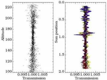
Fig. 3.Transmission is shown as a function of altitude (left) and ap-parent position on the face of the sun (right) for a SAGE II measure-ment event on 21 July 2000. Measuremeasure-ments from the 386 nm wave-length channel are displayed. The vertical axis in the right panel is position along a vertical line bisecting the solar image, represented in arbitrary units from 0 (top of the sun as seen from the spacecraft) to 2 (bottom of sun). The data shown here are for slant paths en-tirely above the atmosphere (minimum altitude is 100 km). At posi-tion approximately 0.9, there is a signature of a large sunspot, which has not been filtered for this demonstration. Variations in transmis-sion away from unity are due to errors in the limb-darkening curve used for calibration, as well as instrument noise. Calibration errors are correlated from scan to scan and are hypothesized to be due to rotation of the scan plane.
The assumption of a one-dimensional, time-independent calibration function, or I0 function, has been used for 26 years in SAGE processing and has produced excellent re-sults. However, further improvement can be obtained by rec-ognizing and correcting for the rotation of the scan track. The rotation of the scan track results in deviations of the measured transmittance that are not due to atmospheric at-tenuation, but rather are due to a slight mismatch between the limb-darkening function obtained from exoatmospheric observations and the solar image sampled along the slightly different scan track of a given in-atmosphere scan. This is es-pecially evident and easy to visualize if the scan track skims the edge of a sunspot, which will be seen in the following example. A spot can be observed in the exoatmospheric cal-ibration data but missing in the in-atmosphere scans, or vice versa. In addition, small variations can be observed even away from sunspots due to granulation, faculae or other fea-tures of the solar photosphere. A mechanism for identifying the presence of sunspots has been a part of SAGE processing for many years but it is not possible to eliminate variations due to other forms of solar inhomogeneity.
4 S. P. Burton et al.: Time-dependent limb-darkening calibration approximately one minute. For the purpose of this
demon-stration, a sunspot has been included that would be filtered in normal processing. In the left panel, the data are shown as a function of altitude. The transmission values cluster around unity because all the observations were taken outside the at-mosphere. Perfect normalization should result in a nearly uniform line of transmission with value of unity, with some random scatter due to instrument noise. The overall scale of the variance is small at all altitudes; however the normaliza-tion is noticeably imperfect. For instance, there is a visibly smaller variance towards the middle of the selected altitude range.
In the right panel of Fig. 3, the same normalized trans-mission values are shown as a function of the position on the sun, or rather, the linear distance along the vertical scan track. The first thing to notice is that the points with great-est deviation from unity have been resolved to the same sun position: these points originate from the unfiltered sunspot. Furthermore, even far from the sunspot, this choice of ab-scissa highlights the differences in calibration from scan to scan, since points at the same sun position are normalized by the same calibration value. In this display, points originating in the same scan are connected by a colored line. This color coding reveals the correlation in the apparent noise from scan to scan, and hints at a time-dependence in the variance. The noise is not random; instead, each scan appears to be a slight perturbation of the previous one. This correlation also ex-plains the pattern in the variation in the left panel. The nor-malization function is an average over all the exoatmospheric scans. The average appears to be more accurate in the middle of the range because there is a continuous, not random, vari-ation, between measurements at higher and lower altitudes, or rather at early and late times.
It is proposed here that the apparent time-dependence and correlation with position on the sun observed in Fig. 3 and other exoatmospheric SAGE measurements is due to a grow-ing mismatch between each scan and the limb-darkengrow-ing function that was derived from measurements up to a minute earlier or later. We hypothesize that the observed time-dependence stems primarily from the rotation of the scan plane due to satellite orbital motion.
In the next section, a model simulation is presented to sup-port the hypothesis that scan plane rotation produces appar-ent noise in the transmission measuremappar-ent. It’s followed in Sect. 2.3 and 2.4 by the description of an algorithm to correct for the effect in SAGE or SAGE-like solar occultation data. Data are presented which show the effect of the correction on SAGE II and SAGE III observations.
2.2 Model simulation of time dependent normalization function
In order to qualitatively confirm that the proposed mecha-nism could be responsible for the observed correlation in the transmission uncertainties, we have modeled the orbital
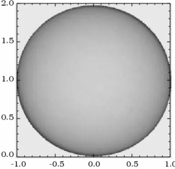
Fig. 4.An 865-nm image of the solar photosphere from the Gas and Aerosol Measurement Sensor, which flew aboard the NASA DC-8 aircraft during the SOLVE II campaign on 21 January 2003. This image was taken at a solar zenith angle of approximately 83.7◦.
geometry and resulting scan patterns. The model combines actual spacecraft and solar ephemeris data from a SAGE II event with a CCD image of the sun obtained from the Gas and Aerosol Measurement Sensor (GAMS) during the sec-ond SAGE-III Ozone Loss Validation Experiment (SOLVE-II) (Pitts et al., 2006). Figure 4 shows a solar image from the GAMS.
0.996 0.998 1.000 1.002 Transmission
0.0 0.5 1.0 1.5 2.0
Sun position
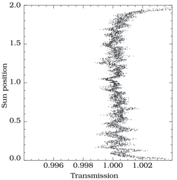
Fig. 5.Simulated transmissions are shown as a function of position on the face of the sun. The biases in transmission near the edges of the sun result from faulty edge matching, due to the image of the sun not being round. Since all scan data are generated from the same image, deviations from one (except at the edges) are indicative of the amount of variation that can be expected from rotation of the scan plane alone.
The calculated transmissions are shown in Fig. 5. Al-though the simulation described here is a rough experiment and there are notable differences between the GAMS imag-ing and the measurement environment of SAGE instrument, the visual similarity of the transmission variations here to those of actual SAGE II events is striking. This supports the idea that the rotation of the scan track is a likely cause of a significant proportion of the observed variance.
2.3 A first-order correction method
In the previous section we noted that the noise pattern in un-binned SAGE transmissions is consistent with rotation of the scan track with respect to features on the face of the Sun. Time series showing the transmission for selected positions along the scan track are shown in Fig. 6. The transmission shown here is normalized by theI0function as usual and then normalized again by a “best guess” transmission profile de-rived by the same averaging and smoothing process as in the standard production process. This renormalization isolates the time-dependent part of the transmission measurements, thereby approximating the time-dependent functionf (actu-ally 1/f) introduced in Eq. (2). The derived error function is shown in Fig. 6 as a function of scan number for a few selected sun position values. Each scan does not sample ex-actly the same positions along the scan track, so the data were
Fig. 6.Transmission, calculated by normalizing the SAGE II mea-surements against the exoatmospheric meamea-surements, and then re-normalized for this experiment by dividing by an average transmis-sion profile, is shown as a function of scan number. The measure-ment event shown here occurred on 1 May 1989. The panels show the transmission within a narrow range of Sun position for chan-nels 1 and 7. Specifically, frames(a)–(c)show channel 1 (1020 nm) for Sun positions 0.5, 1.0, and 1.5, respectively while frames(d)
through(f)show channel 7 (386 nm) for the same Sun positions. Broad scale variation, highlighted by overlaid quadratic fits, is at-tributed to apparent changes in the solar structure (granulation, solar faculae) due to movement of the scan track over the course of the event.
splined onto a grid in sun position to create Fig. 6. Because of the difficulty in creating an accurate transmission vs. al-titude profile in the lower stratosphere and troposphere, the error function values are only shown down to approximately 40 km. For this altitude range, the variation in the error func-tion is well captured by quadratic funcfunc-tions, which are also plotted in Fig. 6. The next section will use an alternative way to approach the isolation of the effects of the variation in the scan track from the actual atmospheric transmission, which is to represent the time-dependent function as a residual, that is, an additive function rather than a multiplicative function. Accordingly,
Ttrue(z)=I (z,p,t )/I0(p)+e(t,p) (3) whereTtrue represents the true transmission; e (t,p) is an “error” variable; and the other variables are as in Eqs. (1) and (2). The “error” variable is the time dependent part, and is the difference between the true transmission and the calculated transmission, that is, measured counts divided by the one-dimensional calibration function (I /I0). Combining Eq. (3) with Eq. (2) shows the relationship between the error variable and the time dependent I-zero correction,f (t,p)
f= 1+ e
I I0
!
6 S. P. Burton et al.: Time-dependent limb-darkening calibration
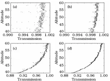
Fig. 7. Unbinned transmission is shown as a function of altitude between 40 and 60 km for SAGE II channels 1 (1020 nm) and chan-nel 7 (386 nm). Frames(a)and(b)show uncorrected and corrected channel 1 while frames(c)and(d)show uncorrected and corrected channel 7. Left and right panels depict transmission before and af-ter the correction, respectively. The specific SAGE II measurement event shown here occurred on 1 May 1989.
In either case, we approximate the function,eorf,by using a best guess transmission in place ofTtrue(z). Simple fits to the error function are then substituted back in to produce the time-dependent correction. In the simple method, the cor-rection is applied by multiplyingT byf, although in a full solution the correction is applied specifically to theI0part. Results using the quadratic fits described above are shown in Fig. 7 for a test event from 1 May 1989. Comparison of the left and right panels in this figure show a conspicuous decrease in the variance in the unbinned transmission, espe-cially in the 386 nm channel (bottom panels).
This relatively simple approach demonstrates the feasibil-ity of correcting forI0 for time-dependent changes. How-ever, some of the simplifications are not optimal for use in the SAGE data processing scheme. For instance, we felt that splining onto a grid in sun position and the use of a global quadratic fit introduce unnecessary error. A more ro-bust modification of this method has been implemented in routine data production and is described in the next section. 2.4 A second-order method
The following algorithm was implemented for SAGE III ver-sion 4.0 data processing (e.g. Thomason et al., 2009) and for a planned SAGE II version 6.3. Our goal was to remove as much variation correlated with position on the Sun as possi-ble while minimizing the risk of being unapossi-ble to separate the effects of the rotating scan track from real atmospheric vari-ability. Accordingly, we moved the cutoff down to 25 km, and thereby used more measurements in each fit. After sub-traction of the altitude based transmission profile from the
Fig. 8. Unbinned transmission is shown in the ozone channel (600 nm) between 40 and 60 km after all other transmission process-ing. In frame(a), no time-dependentI0correction was made, while data in frame(b)employs the correction as described in Sect. 3.4. The measurement event depicted here occurred on 1 May 2005 at (36.0◦N, 58.8◦E).
individual transmission measurements to produce the error function, represented in Eq. (3), local fits were calculated for each measurement point based on nearest neighbors in a combined time and sun-position space. That is, for each point in each scan, a set of neighbors is defined which are the error function estimates for points that are close together in time and linear distance along the scan (sun position). A local fit, cubic in both variables with cross terms, is calcu-lated on the neighbors of each point in each scan and applied only to that single point. By applying the fits only locally, we minimize systematic errors which might otherwise result from using a small-order fit. Fitting in the two-dimensional space, using the sun position variable in addition to the time variable, dispenses with the necessity of splining the mea-surements onto a grid, so no loss of accuracy is introduced in that way.
The time dependentI0correction for each measurement, f (t,p), is derived from the fits using Eq. (4), and then ap-plied to the calculatedI0function as in Eq. (2). With the new calibration function, Level 1 processing is iterated. Figure 8 shows the effect of the full correction on an event that oc-curred on 1 May 2005. The final transmission is shown just before the data are binned to produce a profile. The standard deviation is 30–50% smaller in most bins above 50 km. This is visible in the figure as a clear reduction in the scatter in the corrected case. Below about 50 km, where there begins to be a measurable signal, the uncorrected variance is already smaller, but the corrected data is still noticeably smoother.
0.0001
0.0010
0.0100
Mean Relative Transmission Error
20
40
60
80
100
Altitude (km)
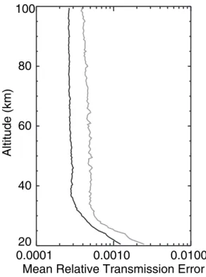
Fig. 9.Mean short wavelength transmission error for approximately 400 sunset events in October 2003 for Version 4 (black) and Ver-sion 3 (grey). The uncertainty is reduced by approximately 40%. The calibration correction described in this paper accounts for about half of the overall reduction.
reduction, but varies from channel to channel, due to varia-tion in the relative importance of solar granularity at different wavelengths. Other factors include improved refraction cal-culations (at low altitudes) and improved scan registration. The final ozone product is also improved in Version 4 due to reduction in the noise. We find that the useable extent of the SAGE III ozone profiles increases by nearly a scale height from 55 km in Version 3 to above 60 km in Version 4 as the overall ozone measurement uncertainty was reduced by about a factor of 2. The calibration correction described here is responsible for an approximately 30% reduction in the ozone uncertainty.
Because of the better match between each measurement and the new calibration function, the time dependentI0 cor-rection improves other parts of the Level 1 processing includ-ing the algorithms responsible for aligninclud-ing scans and locatinclud-ing the edges of the solar disk. In this way, the time dependent correction also affects measurements at altitudes lower than the 25 km cutoff. However, it is above the cutoff where the correction works to greatest effect. Below this level, we use the last correctedI0available from above 25 km.
Although the correction was possible and seemed unbi-ased in some tests penetrating down to just a few kilometers above the tropopause, the more conservative cutoff of 25 km has been adopted for SAGE III Version 4 and the future
SAGE II version 6.3 to more confidently avoid the introduc-tion of systematic error. We have retained the cutoff for two reasons. Firstly, although the error function is defined as the deviation between the calculated and true transmission, in practice the “true” transmission must be approximated. Specifically, we use a “best guess” profile, constructed by smoothing the data using a boxcar average and a running median, the same algorithm that is used to generate the fi-nal profile from the transmission scatter data. It is possible that errors in the best guess transmission profile could lead to errors in the time dependent correction, and these errors are more likely where the atmosphere has a high degree of natural variability. There is also some risk of falsely “cor-recting” or attempting to correct real atmospheric variability by the method described here. It is possible that future de-velopments will allow the algorithm to distinguish between real atmospheric variability and time dependent calibration errors.
3 Concluding remarks
In this work we have presented evidence that a previously unaddressed source of measurement uncertainty exists in the solar occultation technique. This is the time dependent error in the calibration function due to the small (<10◦
) rotation of the scan plane about the center of the sun over the course of a measurement event. Correcting for this effect in SAGE II and SAGE III observations produces a decrease of 20–50% in the variance of the transmission measurements (before the measurements are combined into a single profile), at high altitudes where the correction is most straightforward to implement. While the improvement is smaller and more difficult to apply in the lower stratosphere and troposphere, we feel that the correction technique and, perhaps more importantly, the realization that this error source exists, holds promise for the further improvement of future solar occultation experiments. Specifically, any solar occultation instrument that is deployed in tandem with a full sun imaging device can reap great benefits in that the correct calibration function for every scan in any orientation will be able to be precisely determined.
Edited by: M. Van Roozendael
References
Chu, W. P., McCormick, M. P., Lenoble, J., Brogniez, C., and Pru-vost, P.: SAGE II inversion algorithm, J. Geophys. Res., 94, 8339–8351, 1989.
8 S. P. Burton et al.: Time-dependent limb-darkening calibration
Hansen, J., Sato, M., Ruedy, R., Lacis, A., Asamoah, K., Beckford, K., Borenstein, S., Brown, E., Cairns, B., Carlson, B., Curran, B., de Castro, S., Druyan, L., Etwarrow, P., Ferede, T., Fox, M., Gaffen, D., Glascoe, J., Gordon, H., Hollandsworth, S., Jiang, X., Johnson, C., Lawrence, N., Lean, J., Lerner, J., Lo, K., Lo-gan, J., Luckett, A., McCormick, M. P., McPeters, R., Miller, R., Minnis, P., Ramberran, I., Russell, G., Russell, P., Stone, P., Tegen, I., Thomas, S., Thomason, L., Thompson, A., Wilder, J., Willson, R., and Zawodny, J.: Forcings and chaos in interannual to decadal climate change, J. Geophys. Res., 102, 25679–25720, 1997.
Mauldin III, L. E., Zaun, N. H., McCormick Jr., M. P., Guy, J. H., and Vaughn, W. R.: Stratospheric Aerosol and Gas Experiment II instrument: a functional description, Opt. Eng., 24, 307–312, 1985.
McCormick, M. P., Thomason, L. W., and Trepte, C. R.: Atmo-spheric effects of the Mount Pinatubo eruption, Nature, 373, 399–404, 1995.
Pitts, M. C., Thomason, L. W., Zawodny, J. M., Wenny, B. N., Liv-ingston, J. M., Russell, P. B., Yee, J.-H., Swartz, W. H., and Shet-ter, R. E.: Ozone observations by the Gas and Aerosol Measure-ment Sensor during SOLVE II, Atmos. Chem. Phys., 6, 2695– 2709, 2006,
http://www.atmos-chem-phys.net/6/2695/2006/.
Randel, W. J. and Wu, F.: A stratospheric ozone profile data set for 1979–2005: Variability, trends, and comparisons with column ozone data, J. Geophys. Res., 112, D06313, doi:10.1029/2006JD007339, 2007.
SAGE III ATDB 2002, SAGE III Algorithm Theoretical Basis Doc-ument: Solar and Lunar Algorithm, Earth Observing System Project science Office web site (http://eospso.gsfc.nasa.gov).
Solomon, S., Portmann, R. W., Garcia, R. R., Randel, W., Wu, F., Nagatani, R., Gleason, J., Thomason, L., Poole, L. R., and Mc-Cormick, M. P.: Ozone depletion at mid-latitudes: Coupling of volcanic aerosols and temperature variability to anthropogenic chlorine, Geophys. Res. Lett., 25, 1871–1874, 1998.
Solomon, S., Borrmann, S., Garcia, R. R., Portmann, R., Thomason, L., Poole, L. R., Winker, D., and McCormick, M. P.: Heteroge-neous chlorine chemistry in the tropopause region, J. Geophys. Res., 102, 21411–21429, 1997.
SPARC. 2006: Assessment of Stratospheric Aerosol Proper-ties (ASAP), SPARC Report No. 4, WCRP-124, WMO/TD-No. 1295, edited by: Thomason, L. and Peter, T., February, 2006. Steinbrecht, W., Claude, H., Sch¨onenborn, F., McDermid, I. S., Leblanc, T., Godin, S., Song, T., Swart, D. P. J., Meijer, Y. J., Bodecker, G. E., Connor, B. J., K¨ampfer, N., Hocke, K., Calisesi, Y., Schneider, N., de la No¨e, J., Parrish, A. D., Boyd, I. S., Br¨uhl, C., Steil, B., Giorgetta, M. A., Manzini, E., Thomason, L. W., Zawodny, J. M., McCormick, M. P., Russell III, J. M., Bhartia, P. K., Stolarski, R. S., and Hollandsworth-Frith, S. M.: Long-term evolution of upper stratospheric ozone at selected stations of the Network for the Detection of Stratospheric Change (NDSC), J. Geophys. Res., 111, D10308, doi:10.1029/2005JD006454, 2006. Stenchikov, G., Kirchner, I., Robock, A., Graf, H.-F., Antuna, J., Grainger, R., Lambert, A., and Thomason, L.: Radiative forcing from the 1991 Mount Pinatubo volcanic eruption, J. Geophys. Res., 103, 13837–13857, 1998.
Terao, Y. and Logan, J. A.: Consistency of time series and trends of stratospheric ozone as seen by ozonesonde, SAGE II, HALOE, and SBUV(/2), J. Geophys. Res., 112, D06310, doi:10.1029/2006JD007667, 2007.