Alternative fidelity measure between quantum states
Paulo E. M. F. Mendonça,1,
*
Reginaldo d. J. Napolitano,2,†Marcelo A. Marchiolli,3,‡ Christopher J. Foster,1,§and Yeong-Cherng Liang4,储1
Department of Physics, The University of Queensland, Queensland 4072, Australia 2
Instituto de Física de São Carlos, Universidade de São Paulo, Caixa Postal 369, 13560-970, São Carlos, SP, Brazil 3
Instituto de Física Teórica, Universidade Estadual Paulista, Rua Pamplona 145, 01405-900, São Paulo, SP, Brazil 4
School of Physics, The University of Sydney, NSW 2006, Australia
共Received 18 July 2008; published 19 November 2008兲
We propose an alternative fidelity measure共namely, a measure of the degree of similarity兲between quantum states and benchmark it against a number of properties of the standard Uhlmann-Jozsa fidelity. This measure is a simple function of the linear entropy and the Hilbert-Schmidt inner product between the given states and is thus, in comparison, not as computationally demanding. It also features several remarkable properties such as being jointly concave and satisfying all ofJozsa’s axioms. The trade-off, however, is that it is supermultipli-cative and does not behave monotonically under quantum operations. In addition, metrics for the space of density matrices are identified and the joint concavity of the Uhlmann-Jozsa fidelity for qubit states is established.
DOI:10.1103/PhysRevA.78.052330 PACS number共s兲: 03.67.⫺a, 89.70.Cf
I. INTRODUCTION
The understanding of the set of density matrices as a Rie-mannian manifold 关1兴implies that a notion of distance can be assigned to any pair of quantum states. In quantum infor-mation science, for instance, distance measures between quantum states have proved to be useful resources in ap-proaching a number of fundamental problems such as quan-tifying entanglement关2,3兴, the design of optimized strategies for quantum control 关4,5兴, and quantum error correction
关6–12兴. In addition, the concept of distinguishability between quantum states 关13兴 can be made mathematically rigorous and physically insightful thanks to the close relationship be-tween certain metrics for the space of density matrices and the error probability arising from various versions of the quantum hypothesis-testing problem关14兴. Distance measures are also regularly used in the laboratory to verify the quality of the produced quantum states.
A widely used distance measure in the current literature
共or, more precisely, afidelity measure—that is, a measure of the degree of similarity—between two general density matri-ces兲, is the so-calledUhlmann-Jozsa fidelityF. Historically, this measure had its origins in the 1970s through a set of works by Uhlmann and Alberti 关15–18兴, who studied the problem of generalizing the quantum mechanical transition probability to the broader context of
*
-algebras. The use of the termfidelityto designate Uhlmann’s transition probabil-ity formula is much more recent and initiated in the works of Schumacher 关19兴 and Jozsa 关20兴. Indeed, in an attempt to quantify the degree of similarity between a certain mixed state and a pure state兩典, Schumacher dubbed thetransi-tion probability具兩兩典the fidelity between the two states. In parallel, Jozsa recognized Uhlmann’s transition probabil-ity formula as a sensible extension of Schumacher’s fidelprobabil-ity, where now the measure of similarity is related to a pair of mixed statesand. Ever since, Uhlmann’s transition prob-ability formula has been widely accepted as the generaliza-tion of Schumacher’s fidelity.
The prevalence of this measure as one of the most used notions of distance in quantum information is not accidental, but largely supported on a number of required and desired properties for the role. For example,Fsatisfies all ofJozsa’s axioms; that is, besides recovering Schumacher’s fidelity in the case where one of the states is pure, the following three additional properties also hold: First, F equals unity if and only if it is applied to two identical states; in other cases, it lies between 0 and 1. Second, it is symmetric; i.e., the fidel-ity between and is the same as that between and. Third, it is invariant under any unitary transformation on the state space. Nevertheless,Fisnotthe unique measure satis-fying these properties. A prominent alternative which also complies with Jozsa’s axioms and shares many other proper-ties ofFis given by the nonlogarithmic variety of the quan-tum Chernoff boundQ, recently determined in Ref.关21兴. In analogy with its classical counterpart 关22兴, the quantum Chernoff bound determines—in the limit of asymptotically many copies—the minimum error probability incurred in dis-criminating between two quantum states关21,23兴.
Despite fulfilling the properties listed above, both Fand
Q are, in general, unsatisfying measures from a practical computational viewpoint. AlthoughFcan be expressed in a closed form in terms ofand, it involves successive com-putation of the square roots of Hermitian matrices, which often compromises its use in analytical computations and numerical experiments, especially when the fidelity measure must be computed many times. Even more serious is the case ofQ, which to date has only been defined variationally as the result of an optimization problem 关23兴. The question that naturally arises is whether an easy-to-compute generalization of Schumacher’s fidelity can be obtained. In this paper, we *mendonca@physics.uq.edu.au
†
reginald@ifsc.usp.br ‡
mamarchi@ift.unesp.br §
foster@physics.uq.edu.au 储
provide a positive answer to this question and a thorough analysis of our proposed alternative fidelity measureFN.
Recently, we became aware of the very recent work of Miszczaket al.关24兴in whichFNwas introduced as an upper bound to the Uhlmann-Jozsa fidelity. In many ways our analysis of FN is complimentary to that provided in Ref.
关24兴; results in common are noted in the corresponding sec-tions of our paper.
Our paper is structured as follows. In order to provide a concrete ground for our proposal of FN as an alternative fidelity measure, we first reexamine, in Sec. II, a set of basic properties of the Uhlmann-Jozsa fidelity. In Sec. III we for-mally introduce FNand analyze it in the spirit of the prop-erties reviewed in Sec. II. The computational efficiency of FNis contrasted with a number of previously known distance or fidelity measures in Sec. IV. We summarize our main re-sults and discuss some possible avenues for future research in Sec. V.
II. UHLMANN-JOZSA FIDELITY
In this section, we will briefly survey some physically appealing features inherent to the Uhlmann-Jozsa fidelityF. In Sec. III, these features will be used as a reference for characterizing the proposed fidelity measure.
A. Preliminaries
The Uhlmann-Jozsa fidelity F was originally introduced as a transition probability between two generic quantum states and关15兴:
F共,兲ªmax 兩典,兩典兩具兩典兩
2
=关Tr共
冑
冑
冑
兲兴2. 共1兲
Here,兩典and兩典are restricted to be purifications ofand, while the second equality indicates that the maximization procedure can be explicitly evaluated. At this stage, it is worth noting that it is not uncommon to find
冑
F being re-ferred to, instead, as the fidelity共see, for example, Ref.关22兴兲. In Ref.关20兴, Jozsa conjectured that Eq.共1兲was the unique expression that satisfies a number of natural properties ex-pected for any generalized notion of fidelity 关25兴. Through-out, we shall refer to these asJozsa’s axioms.共1兲 Normalization—i.e., F共,兲苸关0 , 1兴 with the upper bound attained if and only if=共theidentity of indiscern-ible property兲.
共2兲 Symmetry under swapping of the two states—i.e., F共,兲=F共,兲.
共3兲Invariance under any unitary transformationUof the state space—i.e.,F共UU†,UU†兲=F共,兲.
共4兲Consistency with Schumacher’s fidelity when one of the states is pure—i.e.,
F共,兩典具兩兲=具兩兩典 共2兲 for arbitrary and兩典.
The proof that F satisfies all of Jozsa’s axioms follows easily from the variational definition of Eq. 共1兲 共see, e.g., Ref.关22兴for technical details兲. The remainder of this section discusses a number of less immediate properties of F.
B. Concavity properties
The concavity property of quantities like entropy, mutual information, and fidelity measure are often of theoretical in-terest in the quantum information community 关22兴. In this regard, it is worth noting that a useful feature of F is its
separate concavity in each of its arguments; i.e., for p1,p2
艌0,p1+p2= 1, and arbitrary density matrices1,2,1, and
2, we have
F共p11+p22,1兲艌p1F共1,1兲+p2F共2,1兲. 共3兲 By symmetry, concavity in the second argument follows from Eq.共3兲. Separate concavity can be proven关15,20兴using the variational definition ofFfrom Eq. 共1兲.
While it is known that
冑
Fisjointly concave关16,26兴, i.e.,冑
F共p11+p22,p11+p22兲艌p1
冑
F共1,1兲+p2冑
F共2,2兲, 共4兲it is also known that the Uhlmann-Jozsa fidelityFdoesnot, in general, share the same enhanced concavity property关27兴.
C. Multiplicativity under tensor products
Another neat mathematical property ofF共,兲is that it is multiplicative under tensor products: for any density matri-ces1,2,1, and2:
F共1丢2,1丢2兲=F共1,1兲F共2,2兲. 共5兲 This identity follows easily from the following facts: for any Hermitian matrices AandB,共i兲Tr共A丢B兲= Tr共A兲Tr共B兲and
共ii兲
冑
A丢B=冑
A丢冑
B.An immediate consequence of this result is that for two physical systems, described by and, a measure of their degree of similarity given by F remains unchanged even after appending each of them with an uncorrelated ancillary state —i.e.,F共丢,丢兲=F共,兲.
D. Monotonicity under quantum operations
Given that F共,兲 serves as a kind of measure for the degree of similarity between two quantum states and , one might expect that a general quantum operation E will make them less distinguishable and, hence, more similar ac-cording to F关22兴:
F„E共兲,E共兲…艌F共,兲. 共6兲 Indeed, it is now well known that Eq.共6兲holds true关18兴for an arbitrary quantum operation described by a completely positive trace-preserving 共CPTP兲 map E:哫E共兲. Inequal-ity 共6兲 qualifies F as a monotonically increasing measure
under CPTP maps and can be considered the quantum analog of the classical information-processing inequality—which expresses that the amount of information should not increase via any information processing.
maps 关28兴. Clearly, since
冑
F satisfies all the above-mentioned conditions, Eq. 共6兲also follows by simply squar-ing the correspondsquar-ing monotonicity inequality for冑
F.E. Related metrics
The Uhlmann-Jozsa fidelity by itself is not a metric共for a quick review of metrics, see Appendix A兲. However, one may well expect that a metric, which is a measure of dis-tance, can be built up from a measure of similarity such asF. Indeed, the functionals
A关F共,兲兴ªarccos关
冑
F共,兲兴, 共7兲B关F共,兲兴ª
冑
2 − 2冑
F共,兲, 共8兲C关F共,兲兴ª
冑
1 −F共,兲 共9兲 exhibit such metric properties共see Refs.关22,31–35兴and also Appendix B 3 for more details兲. In particular, these function-als are now commonly known in the literature, respectively, as theBures angle关22兴, theBures distance 关32,33兴, and thesine distance关35兴.
F. Trace distance bounds
An important distance measure in quantum information is the metric induced by the trace norm 储·储tr, which is com-monly referred to as the trace distance关22兴:
D共,兲=1
2储−储tr. 共10兲 The trace distance is an exceedingly successful distance mea-sure: it is a metric 共as is any distance induced by norms兲, unitarily invariant关36兴, jointly convex关22兴, decreases under CPTP maps关37兴, and in the qubit case, is proportional to the Euclidean distance between the Bloch vectors in the Bloch ball. The trace distance is also closely related to the minimal probability of error on attempts to distinguish between a single copy of two nonorthogonal quantum states 关38兴. For all of these reasons, one is generally interested to determine how other distance measures relate with the trace distance.
The following functions of the Uhlmann-Jozsa fidelity were shown in Ref.关39兴to provide tight bounds forD关40兴: 1 −
冑
F共,兲艋D共,兲艋冑
1 −F共,兲. 共11兲 In fact, the stronger lower bound 1 −F艋Dholds ifandhave support on a common two-dimensional Hilbert space
关41兴 共e.g., any pair of qubit states兲 or if at least one of the states is pure关22兴.
From these inequalities, one can conclude a type of quali-tative equivalence between the Uhlmann-Jozsa fidelityFand the trace distance D: whenever F is small, D is large and wheneverFis large, Dis small.
III. ALTERNATIVE FIDELITY MEASURE
A. Preliminaries
We shall now turn attention to our proposed measure of the degree of similarity between two quantum states and
—namely,
FN共,兲= Tr共兲+
冑
1 − Tr共2兲冑
1 − Tr共2兲. 共12兲This is simply a sum of the Hilbert-Schmidt inner product betweenandand the geometric mean between their lin-ear entropies. It is worth noting that the same quantity—by the name superfidelity—has been independently introduced in Ref.关24兴as an upper bound for F.
Remarkably, when applied to qubit states,FNis precisely the same asF. This observation follows easily from the fact that for density matrices of dimension d= 2, it is valid to write
兩FN共,兲兩d=2= Tr共兲+ 2
冑
det共兲冑
det共兲, 共13兲which is just an alternative expression of Ffor qubit states
关33,42兴.
Whend⬎2, however,FNno longer recoversF, but can be seen as a simplified version of the fidelity measure pro-posed by Chen and collaborators 关43兴, which reads as
FC共,兲=1 −r
2 +
1 +r
2 FN共,兲, 共14兲
wherer= 1/共d− 1兲anddis the dimension of the state space of and . Moreover, it is straightforward to verify that while FN reduces to the Schumacher’s fidelity 关the right-hand side of Eq.共2兲兴when one of the states is pure; the same cannot be said forFC.
It is not difficult to see from Eq. 共12兲 that FN satisfies Jozsa’s axioms 2, 3, and 4 as enumerated in Sec. II A. The non-negativity ofFNrequired by axiom 1 is also immediate from the definition. As a result, FN is an acceptable gener-alization of Schumacher’s fidelity according to Jozsa’s axi-oms if the following proposition is true.
Proposition III.1.FN共,兲艋1 holds for arbitrary density matrices and, with saturation if and only if=.
Proof.To begin with, recall that anyd⫻ddensity matrix can be expanded in terms of an orthonormal basis of Hermit-ian matrices兵vk其
k=0 d2−1
such that Tr共vivj兲=␦ij共see, for example,
Refs. 关44,45兴兲. In particular, if we let ⌼ជª共v0, . . . ,vd2−1兲, then andadmit the following decomposition:
=rជ·⌼ជ and=sជ·⌼ជ, 共15兲
whererជandsជare real vectors withd2entries共corresponding to the expansion coefficients which can be determined using the orthonormality condition兲. Since and are density matrices, rជ and sជ satisfy 0艋rជ·sជ艋1 and r,s艋1, where r
=储rជ储ands=储sជ储.
Using the expansion of Eq.共15兲in Eq.共12兲, we arrive at the following alternative expression ofFN,
fN共rជ,sជ兲=rជ·sជ+
冑
1 −r2冑
1 −s2 共16兲=Rជ·Sជ, 共17兲
where, in the second line, we have defined two unitvectors inRd2+1
Rជª共rជ,
冑
1 −r2兲 andជSª共sជ,冑
1 −s2兲. 共18兲The normalization of Rជ and Sជ implies that FN共,兲=Rជ·Sជ
艋1, with saturation if and only if Rជ=Sជ, or equivalently
=. 䊏
B. Concavity properties
As with
冑
F, the measureFNis jointly concave in its two arguments; i.e., for p1,p2艌0,p1+p2= 1, and arbitrary den-sity matrices 1,2,1, and2, we haveFN共p11+p22,p11+p22兲
艌p1FN共1,1兲+p2FN共2,2兲. 共19兲
Since F fails to be jointly concave in general, FN has a stronger concavity property. Remarkably, given the equiva-lence betweenF andFNin the d= 2 case, the result of this section implies that F is jointly concave when restricted to qubit states.
The rest of this section concerns a proof of this concavity property of FN. We start by proving the following lemma, which provides a useful alternative expression of inequality
共19兲.
Lemma III.1. Define a function F:关0 , 1兴→Rby
F共x兲ª共rជ+xuជ兲·共sជ+xvជ兲+
冑
1 −储rជ+xuជ储2冑
1 −储sជ+xvជ储2.共20兲
Given the density matrices 1, 2, 1, and 2, there exist vectorsrជ,sជ,uជ,vជ苸Rd
2
andx苸关0 , 1兴such that the inequality
F共x兲艌共1 −x兲F共0兲+xF共1兲 共21兲
is equivalent to Eq. 共19兲.
Proof.The proof is by construction. Using the parametri-zation of Eq.共15兲for the density matrices in inequality共19兲, we obtain the following equivalent inequality for the vectors
r
ជiandsជi:
fN共p1rជ1+p2rជ2,p1sជ1+p2sជ2兲艌p1fN共rជ1,sជ1兲+p2fN共rជ2,sជ2兲,
共22兲
where the function fNwas defined in Eq. 共16兲.
A straightforward computation shows that inequality共21兲
is identical to inequality共22兲 when we identifyx⬅p2, 1 −x
⬅p1, and set
r
ជ=rជ1, uជ=rជ2−rជ1,
s
ជ=sជ1, vជ=ជs2−sជ1. 共23兲
IfF共x兲has negative concavity inx苸关0 , 1兴, then inequal-ity 共21兲 is automatically satisfied as it establishes that the straight line connecting the points(0 ,F共0兲)and(1 ,F共1兲)lies below the curve 兵(x,F共x兲)兩x苸关0 , 1兴其. As a result, the joint concavity ofFNis proved with the following proposition.
Proposition III.2. For x苸关0 , 1兴, andrជ,sជ,uជ,vជ苸Rd
2 speci-fied in Eq. 共23兲, the functionF共x兲 关cf. Eq.共20兲兴satisfies
d2F共x兲
dx2 艋0 共24兲
and hence FNis jointly concave.
The proof of this proposition is given in Appendix B 1.
C. Multiplicativity under tensor products
In contrast with F, the measureFN is not multiplicative under tensor products. In fact, it is generally not even invari-ant under the addition of an uncorrelated ancilla prepared in the state. In this case,FNbetween the resulting states reads as
FN共丢,丢兲
= Tr共兲Tr共2兲
+
冑
1 − Tr共2兲 Tr共2兲冑
1 − Tr共2兲 Tr共2兲
, where the left-hand side equals FN共,兲 if and only if Tr共2兲
= 1 or, in other words, if and only ifis a pure state. More generally, it can be shown that FNis supermultiplica-tive, i.e.,
FN共1丢2,1丢2兲艌FN共1,1兲FN共2,2兲. 共25兲 A proof of this property is given in Appendix B 2; a similar proof was independently obtained in Ref.关24兴.
D. Monotonicity under quantum operations
That FN is only supermultiplicative may be a first sign that it may not behave monotonically under CPTP maps. In fact, as we shall see below, Ozawa’s counterexample关46兴to the claimed monotonicity of the Hilbert-Schmidt distance
关47兴can also be used to show thatFNdoes not behave mono-tonically under CPTP maps.
Let˜and˜ be two two-qubit density matrices, written in the product basis as
˜ =1 2
冢
1 0 0 0 0 1 0 0 0 0 0 0 0 0 0 0
冣
and˜ =1 2
冢
0 0 0 0 0 0 0 0 0 0 1 0 0 0 0 1
冣
,
共26兲
and consider the 共trace-preserving兲 quantum operations of tracing over the first or second qubit. A straightforward com-putation shows that if the first qubit is traced over, then
FN„Tr1共˜兲,Tr1共˜兲…= 1⬎ 1
2=FN共˜ ,˜兲, 共27兲 which satisfies the desired monotonicity property. However, if instead the second subsystem is discarded, we find
FN„Tr2共˜兲,Tr2共˜兲…= 0⬍ 1
2=FN共˜ ,˜兲. 共28兲 Together, Eqs. 共27兲and共28兲show thatFN is neither mono-tonically increasing nor decreasing under general CPTP maps.
pro-jective measurements—with the measurement outcomes forgotten—give rise to a higher value ofFNfor the resulting pair of states? An affirmative answer would follow from a proof of the inequality
FN
冉
兺
iPiPi,
兺
iPiPi
冊
艌FN共,兲 共29兲for any complete set of orthonormal projectors Pi and for arbitrary density matrices and.
It is a simple exercise to prove Eq.共29兲for the particular case where either of the commutation rules 关Pi,兴= 0 or
关Pi,兴= 0 is observed for all values ofi. Whether the same conclusion can be drawn for the more general, noncommu-tative cases remains to be seen. In this regard, we note that a preliminary numerical search favors the validity of Eq.共29兲.
E. Related metrics
In parallel to the metrics A关F兴, B关F兴, and C关F兴 intro-duced in Sec. II E, we define
A关FN共,兲兴ªarccos关
冑
FN共,兲兴, 共30兲B关FN共,兲兴ª
冑
2 − 2冑
FN共,兲, 共31兲C关FN共,兲兴ª
冑
1 −FN共,兲, 共32兲 and prove that whileC关FN兴preserves the metric properties, both A关FN兴 andB关FN兴 do not always obey the triangle in-equalityX关FN共,兲兴艋X关FN共,兲兴+X关FN共,兲兴, 共33兲 whereX here refers to eitherA,B, orC. For example, con-sider the qutrit density matrices, =13/3,
=
冢
1 0 0 0 0 0 0 0 0冣
and=
冢
0.90 0.04 0.03 0.04 0.05 0.02 0.03 0.02 0.05
冣
. 共34兲
Numerical computation of the quantities appearing in the triangle inequality gives rise to Table I. Note that for X
=A,B, the first column dominates the second; i.e., the tri-angle inequality is violated and therefore neither A关FN兴nor
B关FN兴is metrics. ForX=C, no violation is observed for the above density matrices. Next, we prove that this is the case for any three density matrices,, and; thus,C关FN兴is a metric.
Proposition III.3. The quantity C关FN共,兲兴 is a metric for the space of density matrices.
To prove this proposition, we will make use of the follow-ing theorem due to Schoenberg关48兴 共see also关49兴, Chap. 3, Proposition 3.2兲. We state here an abbreviated form of the theorem sufficient for our present purposes.
Theorem III.1 (Schoenberg). LetXbe a nonempty set and
K:X⫻X →R a function such that K共x,y兲=K共y,x兲 and
K共x,y兲艌0 with saturation if and only if x=y, for all x,y
苸X. If the implication
兺
i=1 nci= 0⇒
兺
i,j=1 n
K共xi,xj兲cicj艋0 共35兲
holds for alln艌2,兵x1, . . . ,xn其債X, and兵c1, . . . ,cn其債R, then
冑
Kis a metric.We make a small digression at this point to remark that, in spite of its successful application on the grounds of classical probability distance measures 关50–52兴, Schoenberg’s theo-rem has received almost no attention by the quantum infor-mation community. In this paper, besides proving the metric properties ofC关FN兴, we will also make use of Schoenberg’s theorem to provide independent proofs of the metric proper-ties of B关F共,兲兴 andC关F共,兲兴 共see Appendix B 3兲.
Proof of Proposition III.3. Clearly, from the definition of
C2关FN共,兲兴, it is easy to see that it inherits fromFN共,兲
the property of being symmetric in its two arguments and thatC2关F
N共,兲兴艌0 with saturation if and only if=. So, to apply Theorem III.1, we just have to show that for any set of density matrices 兵i其i=1
n 共n
艌2兲 and real numbers 兵ci其i=1 n
such that兺i=1 n
ci= 0, it is true that
兺
i,j=1 nC2关FN共i,j兲兴cicj艋0. 共36兲
This follows straightforwardly by exploiting the zero-sum property of the 共real兲coefficients ciand the linearity of the trace,
兺
i,j=1 n关1 − Tr共ij兲−
冑
1 − Tr共i 2兲冑
1 − Tr共j 2兲兴c
icj
= − Tr
冋
冉
兺
i=1 ncii
冊
2册
−冋
兺
i=1 n
ci
冑
1 − Tr共i 2兲
册
2
艋0,
共37兲
which concludes the proof. 䊏
We note that a proof of the metric property of
冑
2C关FN共,兲兴—by the namemodified Bures distance—was independently provided by Ref. 关24兴. The proof provided above is significantly shorter thanks to the power of Schoe-nberg’s theorem.F. Trace distance bounds
In Sec. II F, we have seen that a kind of qualitative equivalence betweenDandFcan be established through the bounds onDgiven by functions ofF; cf. Eq.共11兲. Here, we will provide similar bounds on D in terms of functions of FN.
Proposition III.4. For any two density matricesandof TABLE I. A numerical test of the triangle inequality forA关FN兴,
B关FN兴, andC关FN兴.
X X关FN共,兲兴 X关FN共,兲兴+X关FN共,兲兴
A 0.9553 0.9241
B 0.9194 0.9137
dimension d, the trace distanceD共,兲satisfies the follow-ing upper bound:
D共,兲艋
冑
r2
冑
1 −FN共,兲, 共38兲 whererªrank共−兲. Moreover, this upper bound onDcan be saturated with states of the form=Udiag关⌳d兴U † Tr共diag关⌳d兴兲
and =Udiag关P共⌳d兲兴U † Tr共diag关⌳d兴兲
,
共39兲
whereUis an arbitrary unitary matrix of dimensiond,⌳dis an ordered list ofdelements taking values in the set兵1,2其
共1,2艌0, but not simultaneously zero兲andP共⌳d兲is the list formed by some permutation of the elements in⌳d.
Proof. Note that the product of square roots in the expres-sion of FN, Eq. 共12兲, is the geometric mean between the linear entropies ofand. It then follows from the inequal-ity of arithmetic and geometric means that
1 − Tr共2兲
2 +
1 − Tr共2兲
2 艌
冑
1 − Tr共 2兲冑
1 − Tr共2兲 ,
共40兲
which can be reexpressed as the following inequality after summation of Tr共兲to both sides:
储−储HS艋
冑
2关1 −FN共,兲兴. 共41兲Here, 储X储HSª
冑
Tr共X†X兲 is the Hilbert-Schmidt norm共also known as Frobenius norm兲, defined for an arbitrary matrixX. The Hilbert-Schmidt norm and the trace norm 储X储trªTr共
冑
X†X兲are related according to关53兴储X储tr艋
冑
x储X储HS, 共42兲 where xªrank共X兲. Used in Eq. 共41兲, the above inequality leads to the desired resultD共,兲=1
2储−储tr艋
冑
r
2
冑
1 −FN共,兲. 共43兲 To prove that the states in Eq.共39兲saturate this bound, we first note that because those states are isospectral, their linear entropies are identical and hence inequality共40兲is saturated. To prove saturation of inequality共42兲, simply use Eq.共39兲to compute储−储tr= Tr关
冑
共−兲2兴=r兩1−2兩 Tr共diag关⌳d兴兲
, 共44兲
储−储HS=
冑
Tr关共−兲2兴=冑
r兩1−2兩 Tr共diag关⌳d兴兲, 共45兲
from which the identity 储−储tr=
冑
r储−储HS isimmedi-ate. 䊏
How good are these upper bounds? With some thought, it is not difficult to conclude that the states arising from Eq.
共39兲can only have evenrand are thus unable to saturate the upper bound of Eq. 共38兲 for odd r. Nonetheless, from our
numerical studies, it seems like the absolute upper bound— corresponding to the choice r=d on the right-hand side of Eq. 共38兲—is actually unachievable byanystates ifd is odd. An illustration of this peculiarity can be seen in Fig. 1共a兲, where the upper bound corresponding to r= 3 is well sepa-rated from the region attainable by physical states. In con-trast, for every even d, the states given by Eq.共39兲do trace out a tight boundary for the region attainable with physical states, as shown in Fig.1共b兲for d= 6.
On the other hand, it can also be seen from Fig.1that no points occur in the region where D艋1 −FN. Indeed, inten-sive numerical studies ford= 3 , 4 , . . . , 50 have not revealed a single pair of density matrices which contributed to a point in this region. This suggests that the following lower bound onD, in terms ofFN, may well be established.
Conjecture III.1. The trace distanceD共,兲and the mea-sureFN共,兲 between two quantum states andsatisfy
(a)
(b)
FIG. 1. 共Color online兲Plot of the trace distanceD共,兲 vs 1
−FN共,兲 for 4⫻106pairs of randomly generated and with
共a兲d= 3 and共b兲d= 6. The darker共blue兲points are generated using pairs of mixed states whereas the lighter共green兲points are gener-ated using at least one pure state. The antidiagonal solid line is the conjectured lower bound, whereas the upper bounds given by Eq.
D共,兲艌1 −FN共,兲. 共46兲 In relation to this, it is also worth noting that the following
共weaker兲lower bound can readily be established via a recent result given in Ref. 关24兴:
Proposition III.5. The trace distanceD共,兲and the mea-sure FN共,兲between two quantum states andsatisfy the inequality
D共,兲艌1 −
冑
FN共,兲. 共47兲Proof. This lower bound onDfollows immediately from the lower bound on D given in inequality 共11兲 and the in-equalityF艋FNrecently established in Ref.关24兴. 䊏 As with the Uhlmann-Jozsa fidelityF, we can thus infer that whenever FN is large enough, D is close to zero and whenever FN is close to zero, D is close to unity. However—as should be clear from Fig. 1共b兲—the converse implication is not necessarily true.
IV. COMPUTATIONAL EFFICIENCY
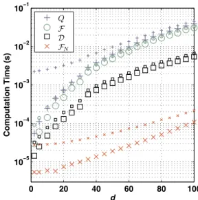
For two general density matrices and , analytical evaluation of the Uhlmann-Jozsa fidelity F共,兲 can be a formidable task. This is in sharp contrast with FN共,兲, which involves only products and traces of density matrices. Even at the numerical level—due to the complication in-volved in evaluating the square root of a Hermitian matrix— the computation of F共,兲can be rather resource consum-ing. For a quantitative understanding of the computational efficiency, we have performed a numerical comparison of the time required to calculate the fidelity measuresFandFN, the nonlogarithmic variety of the quantum Chernoff bound Q, and the trace distanceD. We have implemented the compu-tations in both Matlab and C; we present the Matlab codes for reasons of accessibility and succinctness, while the C codes provide accurate timings without the overhead of the Matlab interpreter.
The time required to evaluate each function was estimated by averaging the times for 100 pairs of randomly generated
d-dimensional density matrices 关54兴. Results are shown in Fig.2as a function ofd. The Matlab codes are presented in Appendix C; we attempted to make these codes as efficient as possible within the constraints of the Matlab environment. Corresponding C codes were implemented as Matlab MEX-files for convenience and can be found online 关56兴. Our C implementation directly calls the LAPACK and BLAS librar-ies included in the Matlab distribution for eigenvalue decom-positions and matrix operations. The minimization required in the computation ofQwas performed using the Brent mini-mizer from the GNU Scientific Library关57兴.
The results shown in Fig. 2 are consistent with the ex-pected algorithmic complexity: Both F and Q require two Hermitian diagonalizations, taking an expectedO共d3兲 opera-tions each关58兴. ComputingQis the slowest since it requires both sets of eigenvectors, whileFrequires only eigenvalues from one of the diagonalizations. Next fastest is the compu-tation of D which requires only eigenvalues from a single diagonalization. All of F, Q, and D appear to require an asymptotic O共d3兲 operation because of the necessity of
di-agonalization or some other method for computing functions of the input matrices. On the other hand, our proposed fidel-ity measure FN requires only three Hilbert-Schmidt inner products, with asymptotic performance O共d2兲. Figure 2
clearly shows that the practical numerical evaluation ofFNis dramatically faster than the evaluation of F,D, or Q. This raises the prospect of using FN as a numerically efficient estimate of distance measures such as F 关24兴 and D—particularly for smalldwhere the bounds proven in Sec. III F are tighter. As the dimension increases, the computa-tional advantage of usingFN becomes even greater, but the quality of the estimate drops.
V. CONCLUDING REMARKS
In this paper, we have proposed the quantity FN as an alternative fidelity measure共namely, a measure of the degree of similarity兲 between an arbitrary pair of mixed quantum states. This measure and the prevailing Uhlmann-Jozsa fidel-ity F and the nonlogarithmic variety of the quantum Cher-noff boundQ关21兴are, to the best of our knowledge, the only known fidelity measures between density matrices that com-ply with Jozsa’s axioms关20兴. That is,F,Q, and FNare the only known measures that generalize to pairs of mixed states the concept of fidelity introduced by Schumacher between a pure and a mixed state关19兴.
The simplicity of FN is in sharp contrast withF andQ
since it involves only products of density matrices. Numeri-cally, this leads to significant reduction in computation time forFN共,兲overF共,兲, especially for higher-dimensional systems.
Besides being easier to compute,FNhas also been shown to preserve共and even enhance兲a number of the useful
prop-0 20 40 60 80 100
10−5 10−4 10−3 10−2 10−1
d
C
omputation
Time
(s
)
Q
F D F
N
FIG. 2. 共Color online兲A semilog plot of the average computa-tion time in Matlab and C for the fidelity measuresF共䊊兲,FN共⫻兲,
the nonlogarithmic variety of the quantum Chernoff boundQ共⫹兲, and the trace distanceD共䊐兲as a function of the dimensiondof the
erties ofFandQ. For example, we have shown thatFNis a jointly concave measure, that it can be used to place upper and lower bounds on the value of the trace distance, and that it gives rise to a new metric for the space of density matrices. A remarkable consequence of the joint concavity of FN is that F is also jointly concave when restricted to a pair of qubit states—an interesting problem which remained un-solved thus far关59,60兴.
Our measure, nevertheless, is not without its drawbacks. To begin with, FN—unlike measures such asFor Q—does not behave monotonically under CPTP maps. In addition, it does not necessarily vanish when applied to any pair of
mixed states, which are otherwise recognized to be com-pletely different according toF,Q, or their trace distanceD. In fact, the explicit dependence on the linear entropies of
and gives rise to the following undesirable feature: the value ofFNbetween two completely mixed states residing in disjoint subspaces can get arbitrarily close to unity as the dimension of the state space tends to infinity.
The undesirable features ofFNprovide a clue as to when FN may not be the preferred measure of similarity between two quantum states: We know thatFNdoes not measure the similarity between two high-dimensional, highly mixed states共i.e., states having non-negligible linear entropy兲in the same way that measures like F, Q, or D would. In these cases, the interpretation of FN as a measure of similarity between quantum states must be carried out with extra cau-tion.
With this in mind, we nevertheless seeFNas an attractive alternative toF. Even when out of its range of applicability, it follows from a very recent result of Miszczak et al.关24兴
that FN provides an upper bound on the Uhlmann-Jozsa fi-delityF. Moreover, it seems promising thatFNbetween any two quantum states may be measured directly in the labora-tory, without resorting to any state tomography protocol关24兴. Let us now briefly mention some possibilities for future research that stem from the present work. To begin with, it would be interesting to search for a quantitative relationship between FN and Q analogous to that between FN and D established in this paper or that betweenFNandFgiven in Ref. 关24兴. An estimate of Q based on some function ofFN would be useful given that a closed form for Q is not cur-rently known and thatFNcan be computed relatively easily. In addition, assuming FN as an alternative to F, it seems reasonable to reexamine some of the problems whereFhas proven useful, but with FN playing its role. In particular, it would be interesting to investigate whether the simplicity associated withFN will offer some advantages overF.
As a first example, we recall from Refs.关2,3兴that a stan-dard measure for the amount of entanglement of a stateis given by the shortestdistancefromto the set of separable density matrices. Given the relative simplicity of FN with respect toF, it is not inconceivable that a distance measure based on FN 共such asC关FN兴兲 may lead to a more efficient determination of this quantity if compared, for example, to
C关F兴or the Bures distance关3兴. Of course, sinceC关FN兴does not satisfy all the sufficient conditions required to give rise to a good entanglement measure 关2兴, any serious attempts in this direction should be preceded by further investigation of the impact of the nonmonotonicity ofFNunder CPTP maps.
For instance, the nonmonotonicity of FN might also imply that the shortest distance from any given stateto the set of separable states—as measured by C关FN兴—does not satisfy the necessary conditions stipulated in Ref. 关61兴, but this is not clear to us at this stage.
As another example,FNcan be used as a figure of merit in designing optimized quantum control and/or quantum er-ror correction strategies: One is typically interested in deter-mining a quantum operation C that minimizes the averaged
distance between the elements of a set of noisy quantum statesiand a predefined set of target quantum statesi. In this context, it would be interesting to investigate if distance measures based onFNwould lead to any advantage in terms of computation time. Clearly, this has potential applications to the implementation of real-time quantum technologies.
Yet another possible direction of research consists of em-ploying FN as a distance measure between quantum operations—as opposed to quantum states—via the isomor-phism between quantum states and CPTP maps 关62,63兴. In this regard, it is worth investigating whether distance mea-sures based onFNwould satisfy the six criteria proposed in Ref. 关34兴. Remarkably, from the results of the present work and Ref. 关24兴, a few strengths of FN-based measures can already be anticipated. Of special significance are the fulfill-ment of the criteria “easy to calculate” and “easy to mea-sure.” Along these lines, some operational meaning for FN would also be highly desirable. Although we do not presently have a compelling physical interpretation of FN, it is not inconceivable that one can be found in an analogous way to F关41兴.
ACKNOWLEDGMENTS
The authors thank Karol Życzkowski, Armin Uhlmann, and an anonymous referee for useful comments on an earlier version of this manuscript. P.E.M.F.M. and Y.C.L. acknowl-edge Sukhwider Singh, Andrew C. Doherty, Alexei Gilchrist, Marco Barbieri, Stephen Bartlett, and Mark de Burgh for helpful discussions. This work is supported by the Brazilian agencies Coordenação de Aperfeiçoamento de Pessoal de Nível Superior 共CAPES兲, Fundação de Amparo à Pesquisa do Estado de São Paulo共FAPESP兲, Project No. 05/04105-5, the Brazilian Millennium Institute for Quantum Information, Conselho Nacional de Desenvolvimento Científico e Tec-nológico 共CNPq兲, and the Australian Research Council.
APPENDIX A: METRICS
From a mathematically rigorous viewpoint, a distance measureDon a setSis a functionD:S⫻S→Rsuch that for every a,b,c苸S the following properties hold.
共M1兲D共a,b兲艌0 共non-negativity兲,
共M2兲D共a,b兲= 0 if and only ifa=b共identity of indiscern-ible兲,
共M3兲D共a,b兲=D共b,a兲 共symmetry兲,
APPENDIX B: PROOFS
1. Proof of Proposition III.2
In this appendix the joint concavity of FNis established via the proof of Proposition III.2.
Proof. Differentiating Eq.共20兲twice with respect tox, we obtain
d2F共x兲 dx2 = 2uជ·
v
ជ+ d 2f共x兲
dx2 g共x兲+f共x兲 d2g共x兲
dx2 + 2 df共x兲
dx dg共x兲
dx ,
共B1兲
where, for convenience, we define the functions f共x兲
ª
冑
1 −储rជ+xuជ储2andg共x兲ª
冑
1 −储sជ+xvជ储2. After somecompu-tation we find that
d2F共x兲
dx2 =F1共x兲+F2共x兲, 共B2兲
where
F1共x兲ª2uជ·vជ−
g共x兲u2 f共x兲 −
f共x兲v2
g共x兲 , 共B3兲
F2共x兲ª2
uជ·共rជ+xuជ兲vជ·共sជ+xvជ兲
f共x兲g共x兲 −
g共x兲关uជ·共rជ+xuជ兲兴2
关f共x兲兴3
− f共x兲关
vជ·共sជ+xvជ兲兴2
关g共x兲兴3 . 共B4兲
The negative semidefiniteness of d2F共x兲/dx2 in the range x 苸关0 , 1兴can be observed ifF1共x兲andF2共x兲are written in the following alternative form:
F1共x兲= −
冐
冑
g共x兲f共x兲uជ−
冑
f共x兲 g共x兲vជ冐
2 ,
F2共x兲= − 1
f共x兲g共x兲冋 g共x兲
f共x兲uជ·共rជ+xuជ兲− f共x兲
g共x兲vជ·共sជ+xvជ兲
册
2 .
䊏
2. Proof of supermultiplicativity ofFN
To prove that FN is supermultiplicative, we first define
riªTr共i 2兲
andsiªTr共i 2兲
, such that 0⬍ri, si艋1 共note that here we useriinstead ofri
2
as the norm square ofrជi, likewise for si兲. Straightforward algebra gives
FN共1丢2,1丢2兲−FN共1,1兲FN共2,2兲
=
冑
共1 −r1r2兲共1 −s1s2兲−冑
共1 −r1兲共1 −s1兲共1 −r2兲共1 −s2兲 − Tr共11兲冑
共1 −r2兲共1 −s2兲− Tr共22兲冑
共1 −r1兲共1 −s1兲. A direct application of Cauchy-Schwarz’s inequality Tr共ii兲艋冑
risigivesFN共1丢2,1丢2兲−FN共1,1兲FN共2,2兲
艌
冑
共1 −r1r2兲共1 −s1s2兲−冑
共1 −r1兲共1 −s1兲共1 −r2兲共1 −s2兲−
冑
r1s1共1 −r2兲共1 −s2兲−冑
r2s2共1 −r1兲共1 −s1兲.The supermultiplicative property is obtained by showing the positive semidefiniteness of the right-hand side of the above expression. This is the content of the following propo-sition.
Proposition B.1. For 0艋a,b,c,d艋1, we have
冑
共1 −ab兲共1 −cd兲艌冑
共1 −a兲共1 −b兲共1 −c兲共1 −d兲+
冑
ac共1 −b兲共1 −d兲+冑
bd共1 −a兲共1 −c兲.共B5兲
Proof. First note that if any of the variables equals 1, then the validity of the inequality is immediate. For example, let
d= 1 so that inequality 共B5兲reduces to
冑
共1 −ab兲共1 −c兲艌冑
b共1 −a兲共1 −c兲. 共B6兲This is trivially satisfied for all 0艋a,b,c艋1. In what fol-lows, we restrict ourselves to 0艋a,b,c,d⬍1 and show that inequality 共B5兲 is equivalent to the standard inequality of arithmetic and geometric means 共hereafter referred as the AM-GM inequality兲. This inequality is just an expression of the fact that the geometric mean of a list of non-negative real numbers is never larger than the corresponding arithmetic mean.
Apply the substitution a
⬘
= 1 −a 共similarly forb⬘
,c⬘
, andd
⬘
; note that 0⬍a⬘
,b⬘
,c⬘
,d⬘
艋1兲to inequality共B5兲and di-vide the result by冑
a⬘
b⬘
c⬘
d⬘
to get the equivalent inequality冑
共1 +A+B兲共1 +C+D兲艌1 +冑
AC+冑
BD, 共B7兲where we have definedA= 1/a
⬘
− 1共similarly for B,C, and D; note that 0艋A,B,C,D⬍ ⬁兲. Squaring the inequality above we findA+C
2 +
B+D
2 +
AD+BC
2 艌
冑
AC+冑
BD+冑
ABCD,共B8兲
which is clearly a sum of three AM-GM inequalities. 䊏
3. Proof of the metric property ofB[F] andC[F]
In the following, we give an alternative demonstration of the metric properties ofB关F兴andC关F兴 共see Refs.关32,34兴for the standard proofs兲. Our proof consists of a simple applica-tion of Theorem III.1 due to Schoenberg.
Proposition B2. The functionals B关F共,兲兴 and
C关F共,兲兴, defined in Eq. 共8兲 and Eq. 共9兲, are metrics for the space of density matrices.
Proof. Let K关F共,兲兴 represent either B关F共,兲兴 or
C关F共,兲兴 for brevity. As with F, it is easy to check that
K2关F共,兲兴 is symmetric in its two arguments and that
K2关F共,兲兴艌0 with saturation if and only if =. So, ac-cording to Theorem III.1,K关F共,兲兴 is a metric if for any set of density matrices兵i其i=1
n 共
n艌2兲and real numbers兵ci其i=1 n
such that兺i=1 n c
兺
i,j=1 nK2关F共i,j兲兴cicj艋0. 共B9兲
To prove this, we derive an upper bound for K2关F共i,j兲兴, which can be easily seen to satisfy the condition above. First, note that
F共i,j兲=关Tr共兩
冑
i冑
j兩兲兴2艌兩Tr共冑
i冑
j兲兩2=关Tr共
冑
i冑
j兲兴2 = Tr共冑
i冑
j丢冑
i冑
j兲 = Tr关共冑
i丢冑
i兲共冑
j丢冑
j兲兴⬅A共i,j兲, 共B10兲
where the first equality follows from the definition
兩A兩ª
冑
A†A for every matrix A and the inequality from the fact that Tr共兩A兩兲= maxU兩Tr共UA兲兩 共the maximization runsover unitary matricesU关20,64兴兲. Then, it follows that
B2关F兴= 2共1 −
冑
F兲艋2共1 −F兲艋2共1 −A兲, 共B11兲C2关F兴= 1 −F艋1 −A艋2共1 −A兲, 共B12兲 or, in our more compact notation, K2关F兴艋2共1 −A兲.
Now, replacingK2关F共i,j兲兴with the above upper bound in the left hand side of Eq. 共B9兲, it is easy to obtain the desired inequality:
兺
i,j=1 n兵2 − 2Tr关共
冑
i丢冑
i兲共冑
j丢冑
j兲兴其cicj= − 2Tr
冉
冏
兺
i=1 nci
冑
i丢冑
i冏
2冊
艋0, 共B13兲where the equality is obtained by using the fact that 兺i=1 n c
i = 0, the linearity of the trace operation, and the hermiticity of
ci
冑
i丢冑
i. 䊏Finally, let us just mention that besides establishing the metric properties of B关F兴 andC关F兴, the present proof also establishes
冑
2 − 2关Tr共冑
冑
兲兴2as a metric for the space of density matrices. In fact, by a similar application of Schoe-nberg’s theorem, the quantityH共,兲ª
冑
2 − 2 Tr共冑
冑
兲can also be shown to be a metric.APPENDIX C: MATLAB CODES
In this appendix, we present the Matlab codes that we have used to compute the various functions involved in the numerical experiment presented in Sec. IV.
For rho and sigma density matrices,
• FNwas computed using
Fn= real共rho共:兲’ⴱsigma共:兲. . .兲 +sqrt共共1 − rho共:兲’ⴱrho共:兲兲ⴱ. . .兲 共共共1 − sigma共:兲’ⴱsigma共:兲兲兲兲;
• Fwas computed using
关V , D兴= eig共rho兲;
sqrtRho= Vⴱdiag共sqrt共diag共D兲兲兲ⴱV’; F = sum共sqrt共eig共Hermitize共. . .兲兲兲兲
共共共共sqrtRhoⴱsigmaⴱsqrtRho兲兲兲兲ˆ2;
Here sqrtRhoⴱsigmaⴱsqrtRho is not quite Hermitian due to small numerical errors. We therefore employ the function Hermitize 共m兲=共M + M
⬘
兲/2 to turn the almost-Hermitianmatrix into a Hermitian one—this causes Matlab to select a more efficient algorithm for the diagonalization.
• Dwas computed using
D = 0.5ⴱsum共abs共eig共rho-sigma兲兲兲; • Qwas computed using
关Vr, Drho兴= eig共rho兲; Dr= diag共Drho兲;
关Vs, Dsigma兴= eig共sigma兲; Ds= diag共Dsigma兲; A = abs共Vr’ⴱVs兲.ˆ2;
关x , Q兴= fminbnd共@共s兲. . .兲
共共Dr. ’ .ˆs兲ⴱAⴱ共Ds.ˆ共1 − s兲兲, 0 , 1兲;
The algorithm used here follows from the formula for Tr共s1−s兲given in the section entitledconvexity in sof Ref.
关21兴.
关1兴I. Bengtsson and K. Życzkowski, Geometry of Quantum States: An Introduction to Quantum Entanglement共Cambridge University Press, Cambridge, England, 2006兲.
关2兴V. Vedral, M. B. Plenio, M. A. Rippin, and P. L. Knight, Phys. Rev. Lett. 78, 2275共1997兲.
关3兴V. Vedral and M. B. Plenio, Phys. Rev. A 57, 1619共1998兲.
关4兴A. M. Brańczyk, P. E. M. F. Mendonça, A. Gilchrist, A. C. Doherty, and S. D. Bartlett, Phys. Rev. A 75, 012329共2007兲.
关5兴P. E. M. F. Mendonça, A. Gilchrist, and A. C. Doherty, Phys. Rev. A 78, 012319共2008兲.
关6兴M. Reimpell and R. F. Werner, Phys. Rev. Lett. 94, 080501
共2005兲.
关7兴A. S. Fletcher, P. W. Shor, and M. Z. Win, Phys. Rev. A 75, 012338共2007兲.
关8兴M. Reimpell, R. F. Werner, and K. Audenaert, e-print arXiv:quant-ph/0606059v1.
关9兴R. L. Kosut and D. A. Lidar, e-print arXiv:quant-ph/ 0606078v1.
关11兴N. Yamamoto and M. Fazel, Phys. Rev. A 76, 012327共2007兲.
关12兴N. Yamamoto, S. Hara, and K. Tsumura, Phys. Rev. A 71, 022322共2005兲.
关13兴C. A. Fuchs, Ph.D. thesis, University of New Mexico, 1995.
关14兴M. Hayashi,Quantum Information: An Introduction共 Springer-Verlag, Berlin, 2006兲.
关15兴A. Uhlmann, Rep. Math. Phys. 9, 273共1976兲.
关16兴P. Alberti and A. Uhlmann, inProceedings of the Second In-ternational Conference on Operator Algebras, Ideals, and their Applications in Theoretical Physics, edited by H. Baum-gartel, G. Laßner, A. Pietsch, and A. Uhlmann 共BSB B. G. Taubner-Verl., Leipzig, 1983兲, pgs. 5—11.
关17兴P. M. Alberti, Lett. Math. Phys. 7, 25共1983兲.
关18兴P. M. Alberti and A. Uhlmann, Lett. Math. Phys. 7, 107
共1983兲.
关19兴B. Schumacher, Phys. Rev. A 51, 2738共1995兲.
关20兴R. Jozsa, J. Mod. Opt. 41, 2315共1994兲.
关21兴K. M. R. Audenaert, J. Calsamiglia, R. Munoz-Tapia, E. Bagan, Ll. Masanes, A. Acín, and F. Verstraete, Phys. Rev. Lett. 98, 160501共2007兲.
关22兴M. A. Nielsen and I. L. Chuang,Quantum Computation and
Quantum Information 共Cambridge University Press,
Cam-bridge, England, 2000兲.
关23兴Formally, the quantum Chernoff bound is defined as 关21兴 QCBªlimn→⬁− log共Pe,min,n兲/n= −ln共Q兲, where Pe,min,nis the
minimum error probabiliy incurred in discriminatingncopies of two given quantum states 丢n, 丢n, and Q
ªmin0艋s艋1Tr共s1−s兲.
关24兴J. A. Miszczak, Z. Puchała, P. Horodecki, A. Uhlmann, and K. Życzkowski, Quantum Inf. Comput. 9, 0103共2009兲.
关25兴Although, as mentioned above, this conjecture can be seen to be false with the counterexample of the nonlogarithmic variety of the quantum Chernoff boundQ, determined in Ref.关21兴. In addition, as we will see in Sec. III A, the measure FN
intro-duced in this paper provides yet another counterexample to this conjecture.
关26兴A. Uhlmann, Rep. Math. Phys. 45, 407共2000兲.
关27兴Note that joint concavity implies separate concavity, but not the other way around. For example, the separate concavity of
冑
F共,兲can be obtained from Eq.共4兲by setting1=2andusing the fact thatp1+p2= 1.
关28兴This follows easily from the Stinespring representation of a CPTP map and from the representation of the partial trace operation given in Refs.关29,30兴.
关29兴A. Uhlmann, Wiss. Z.-Karl-Marx-Univ. Leipzig, Math.-Naturwiss. Reihe 20, 633共1971兲.
关30兴E. A. Carlen and E. H. Lieb, Lett. Math. Phys. 83, 107共2008兲.
关31兴A. Uhlmann, Rep. Math. Phys. 36, 461共1995兲.
关32兴D. Bures, Trans. Am. Math. Soc. 135, 199共1969兲.
关33兴M. Hübner, Phys. Lett. A 163, 239共1992兲.
关34兴A. Gilchrist, N. K. Langford, and M. A. Nielsen, Phys. Rev. A 71, 062310共2005兲.
关35兴A. E. Rastegin, e-print arXiv:quant-ph/0602112v1.
关36兴R. Bhatia, Matrix Analysis, Vol. 169, of Graduate Texts in Mathematics共Springer-Verlag, New York, 1997兲.
关37兴M. B. Ruskai, Rev. Math. Phys. 6, 1147共1994兲.
关38兴C. W. Helstrom, Quantum Detection and Estimation Theory,
Vol. 123, of Mathematics in Science and Engineering 共 Aca-demic Press, New York, 1976兲.
关39兴C. A. Fuchs and J. van de Graaf, IEEE Trans. Inf. Theory 45, 1216共1999兲.
关40兴Both inequalities in Eq.共11兲are saturated if=and also if
andhave orthogonal supports. A less trivial example of satu-ration of the upper bound onDis obtained when bothand
are pure states, whereas the lower bound on D can only be 共nontrivially兲saturated in Hilbert spaces of dimension strictly greater than 2共see Ref.关41兴for an example withd= 3兲. More-over, it is not difficult to show that the equality 1 −F=Dholds true if关,兴= 0andat least one of the states is pure.
关41兴R. W. Spekkens and T. Rudolph, Phys. Rev. A 65, 012310
共2001兲.
关42兴M. Hübner, Phys. Lett. A 179, 226共1993兲.
关43兴J. L. Chen, L. Fu, A. A. Ungar, and X. G. Zhao, Phys. Rev. A 65, 054304共2002兲.
关44兴M. S. Byrd and N. Khaneja, Phys. Rev. A 68, 062322共2003兲.
关45兴G. Kimura, Phys. Lett. A 314, 339共2003兲.
关46兴M. Ozawa, Phys. Lett. A 268, 158共2000兲.
关47兴C. Witte and M. Trucks, Phys. Lett. A 257, 14共1999兲.
关48兴I. J. Schoenberg, Trans. Am. Math. Soc. 44, 522共1938兲.
关49兴C. Berg, J. Christensen, and P. Ressel,Harmonic Analysis on Semigroups共Springer-Verlag, New York, 1984兲.
关50兴F. Topsøe, IEEE Trans. Inf. Theory 46, 1602共2000兲.
关51兴F. Topsøe, http://www.math.ku.dk/~topsoe.
关52兴B. Fuglede and F. Topsøe, http://www.math.ku.dk/~topsoe.
关53兴To see that, assume, for simplicity, thatXis a square matrix of dimensiondand letជ 苸Rdbe the vector with entries
1艌 2 艌¯艌 dcorresponding to the singular values ofX. In addi-tion, letvជ 苸Rdbe the vector with the firstx= rank共X兲 entries
equal to 1 and the remainingd−x entries equal to 0. Then, it follows that 储X储tr=兩ជ·vជ兩, 储X储HS=储ជ储 and
冑
x=储vជ储. In thisframework, inequality 共42兲 is equivalent to Cauchy-Schwarz inequality applied toជ andvជ i.e.,兩ជ·vជ兩艋储ជ储储vជ储.
关54兴Here, we follow the algorithm presented in Ref.关55兴to gener-ated-dimensional quantum states. In particular, the eigenval-ues兵i其id=1of the quantum states were chosen from a uniform distribution on thed-simplex defined by兺ii= 1.
关55兴K.Życzkowski, P. Horodecki, A. Sanpera, and M. Lewenstein, Phys. Rev. A 58, 883共1998兲.
关56兴The C codes implemented as Matlab MEX-files can be found at http://physics.uq.edu.au/people/foster/new_fidelity.html.
关57兴M. Galassi, J. Davies, J. Theiler, B. Gough, G. Jungman, M. Booth, and F. Rossi,GNU Scientific Library Reference Manual
共Network Theory Ltd., Bristol, 2006兲.
关58兴B. N. Parlett, Comput. Sci. Eng. 2, 38共2000兲.
关59兴M. A. Nielsen共private communication兲.
关60兴A. Uhlmann共private communication兲.
关61兴G. Vidal, J. Mod. Opt. 47, 355共2000兲; M. Horodecki, Open Syst. Inf. Dyn. 12, 231共2005兲.
关62兴M. Horodecki, P. Horodecki, and R. Horodecki, Phys. Rev. A 60, 1888共1999兲.
关63兴A. Fujiwara and P. Algoet, Phys. Rev. A 59, 3290共1999兲.