Article
J. Braz. Chem. Soc., Vol. 26, No. 2, 373-380, 2015. Printed in Brazil - ©2015 Sociedade Brasileira de Química 0103 - 5053 $6.00+0.00
A
*e-mail: [email protected]
Colloidal Dispersion Stability: Kinetic Modeling of Agglomeration and Aggregation
Guilherme K. Gonzatti,*,a Paulo A. Netz,b Luana A. Fielc and Adriana R. Pohlmannb
aPrograma de Pós-Graduação em Química and bInstituto de Química, Universidade Federal do Rio Grande do Sul (UFRGS), 91501-970 Porto Alegre-RS, Brazil
cPrograma de Pós-Graduação em Ciências Farmacêuticas, Universidade Federal do Rio Grande do Sul (UFRGS), 90610-000 Porto Alegre-RS, Brazil
In this work we present a simple model for the kinetics of agglomeration and aggregation of colloidal particles. We consider that particles agglomerate rapidly and endothermically forming oligomers. These oligomers can, in turn, aggregate irreversibly, in a process that leads to the destabilization of the colloidal system. As these two processes have very different relative energy activations, they occur in different time-scales: the first step is faster and reaches a state
of quasi-equilibrium. Because of this, the enthalpy change during the agglomeration can be
experimentally determined through the variable temperature multiple light scattering (VTMLS) method. Interestingly, this value is related to the relative kinetic stability of the system and can be used to evaluate the stability of new colloidal compositions. Our results are in qualitative agreement with experimental data of low concentration colloidal dispersions consisted of polymer particles and/or surfactant-coated particles.
Keywords: colloidal stability, kinetic modeling, indefinite self-association, secondary-minimum
Introduction
Colloidal dispersions are composed of microscopic solids suspended in a fluid. These systems occur naturally in many situations in biological processes and have an ever growing importance in many realms of technology and science, be it as drug carriers, paints and inks, self-assembling structures, or model systems for the study of collective behavior of crystal, glasses and gels.1-5
Colloidal systems are, however, inherently thermo-dynamically unstable due to surface effects, as a single solid phase would have lower energy. Yet it is possible for these systems to be kinetically stable, depending on its lifetime. The control of such stability is of great importance in the development of colloidal dispersions for therapeutic uses.6-13 A better understanding of the kinetics involved in
the mechanisms of instability has been the aim of several studies since the early works from Smoluchowski14 up to
more recent and thorough approaches, which consider the influence of the secondary interaction energy minimum15,16
a key feature for self-assembling systems.
As the analysis of colloids kinetics is a vast and complex subject, the many numerical, theoretical and computational studies of colloids kinetics found in the literature give valuable insight on the process and precise results, but are unfortunately not readily suitable for the prediction of colloidal stability, a necessary endeavour.
Though nanotechnology has been used as a strategy to control size distribution of colloidal dispersions granting them increased physical stability, the development of methods for rapid and non-destructive evaluation of this stability remains a challenge for applied material sciences. In this context, variable temperature multiple light scattering (VTMLS) has been recently proposed as a novel method for the rapid determination of the relative stability of colloidal dispersions. Experimentally, the VTMLS approaches subject dispersions of polymer particles and/or surfactant-coated particles of low concentration to thermal stress and measure the intensity of backscattered radiation.1
validity of the assumptions made in the VTMLS analysis by modelling the kinetics of the phenomena and solving numerically the kinetics equations thus obtained.
The remaining of this paper is structured as follows: in the Methodology section, the theoretical bases for the VTMLS are briefly exposed and the kinetic model defined; in Results and Discussions, we present the simulation results and relate them to the experimental results; and in Conclusions we summarise our findings.
Methodology
Theoretical thermodynamical basis and VTMLS analysis
In the VTMLS analysis it is assumed that the destabilization of a colloidal dispersion occurs via a two-step mechanism, illustrated in Figure 1. First the dispersed particles can agglomerate endothermically and reversibly by desorption of some surfactant micelles, forming larger agglomerates. The second and final step is the irreversible aggregation of the particles leading to coalescence of the larger agglomerates, destroying the colloidal dispersion. We emphasise that, according to the International Union of Pure and Applied Chemistry (IUPAC), the agglomeration process is a reversible process in which the particles assemble through weak interactions rather than remaining isolated, whereas aggregation is the irreversible process that leads to phase separation.18
The main idea in the process is that, as two moieties come upon contact, energy is absorbed at the first step, breaking the weak forces between the surfactant micelles and the particles, leading to an intermediate state (oligomer) of higher energy. Part of the energy absorbed is then used to overcome the activation energy of the second step. Thus, systems with higher values of enthalpy change (∆H) during
agglomeration can aggregate faster (due to a lower energy
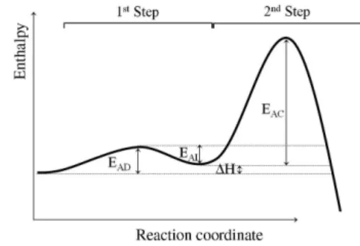
barrier), i.e., have lower kinetic stability. Therefore the enthalpic gain in the first step can be used as an indicative of stability for colloidal dispersions. Figure 2 shows an enthalpy diagram for the process.
A secondary interaction minimum, as depicted in Figure 2, is an extremely important characteristic in colloidal systems, both for thermodynamic properties in self-assembly systems (such as gel-forming colloids) and for the kinetics involved.2-5,19 The role of this secondary minimum is also
more important for interacting particles of greater size.15
The method postulates that the activation energy in the second step is much higher than in the first step. Therefore, the first step is orders of magnitude faster than the second step and, consequently, it can be assumed that a state of thermodynamic quasi-equilibrium can be reached, justifying an analysis through classical thermodynamics.
The classical model of indefinite self-association20
can be used to elucidate the thermodynamics of this equilibrium, as explained below. In this approach, a dispersed particle, i.e., a monomer (A1) can agglomerate
with another monomer forming a dimer (A2), which can
in its turn agglomerate with another monomer, and so on, forming oligomers. This can be represented by Scheme 1:
If the energy change in each of these equilibriums is of similar value, it is reasonable to assume the equilibrium
Figure 1. Illustrative model of the process in aqueous solution. First are depicted the nanosphere monomers (in grey) coated with surfactant. After the first-step agglomeration process oligomers are formed (shown by the dashed line) and some of the surfactant is released. After the second-step aggregation process the oligomers are more closely (and irreversibly) bound and have an even smaller surfactant shell. After this point, the aggregates can flocculate or sedimentate, depending on the density of the solid and fluid phase difference (adapted from reference 1).
Figure 2. Diagram of the enthalpy as a function of the reaction coordinate of the process. EAD is the activation energy for the agglomeration process
in the first step; EAI is the activation energy for the inverse reaction; EAC is the activation energy for the irreversible aggregation (coalescence) and ∆H is the enthalpy change in the first step.
Scheme 1.
1 1 2
A
+
A
A
1 2 3
A
+
A
A
1 i i 1
A
A
A
+
constant has the same value for all of them (EK model). The concentration of each oligomer ([Ai]) is then related to the
equilibrium constant (K) by equation 1. As the temperature influences the value of the equilibrium constant, it will consequently change the concentration profile of oligomers.
[ ]
[ ]
[ ]
[ ]
2 2
2 2 2 2 1
1
A
K A K A
A = ∴ =
[ ]
[ [
] ]
[ ]
[ ]
3 33 3 2 3 1
1 2
A
K A K K A
A A
= ∴ =
2 3
K =K ==K
[
[
[
[
]
]
]
]
]
]
1 1 2 1 i i i i i i K A A K A K A − −= ∴ = (1)
We now define two quantities. The first one is the total concentration of primary particles (CT) which takes
into account all primary particles, whether agglomerated or not (equation 2) and the numerical concentration (CN) which is the total concentration of agglomerates
(equation 3).
[ ] [ ]
1 2 2[ ]
T i
C = A + A ++i A (2)
[ ] [ ]
1 2[ ]
N i
C = A + A + …+ A (3)
The ratio of CN and CT gives us the osmotic coefficient
(ϕ’).20 If K[A1] < 1, it is possible to express ϕ’ as equation 4.
' 1 1 4
2 T N T T KC C C KC
φ = = − ± + (4)
An increase in temperature leads to an increase in the value of K, which in turn causes a decrease of ϕ’. For small
changes of CN there is an approximately linear relation
between ln CN and ln K:
lnK∝−lnCN (5)
The well-known van’t Hoff equation (equation 6) shows the relation of the equilibrium thermodynamic constant with temperature (T):
2 ln ΔH T K RT ∂ = − ∂ (6)
where R is the perfect gas constant. By definite integration between two temperatures, T1 and T2, equation 6 yields
equation 7:
2
1 2 1
ΔH 1 1
ln K
K R T T
= − − (7)
Combining equation 5 and 7 we may write equation 8:
2
1 2 1
ΔH 1 1
ln N N
C A
C R T T
= − (8)
where A is a positive proportionality constant.
In a multiple light scattering analysis the backscattering signal (BS) is related to the differences in the refractive indices and to the photon transport length in the medium (l*),
which is dependent on the particle volume fraction (ϕ) and
the particle size of the dispersed phase (d):20,21
(
)
11 2
* 2 3 1
~ ( ) 2 s g Q BS l d φ − − =
(9)
where Qs is the scattering efficiency factor and g is the
asymmetry factor. Considering that l* ~ CN-1/3, and therefore
BS ~ CN
1/6, it is then possible to combine equations 4, 8 and
9 to relate the backscattering signal to enthalpy changes in the agglomeration, as shown in equation 10:
2
1 2 1
ΔH 1 1
ln BS A'
BS R T T
= − (10)
Experimentally, the VTMLS analysis evaluates the relative stability of colloidal dispersions by measuring the BS of samples subjected to a constant thermal gradient: the samples are heated from 296 to 323 K in 1 h. Even though it is not possible to determine the exact value of
∆H, it is possible to determine the value of A’∆H and to
compare its value for several formulations. It was found, as confirmed by the ageing test, that formulations where these values are higher are the less stable, as shown in Figure 3.
It is important to remark that this approach is only possible by assuming that the agglomeration is sufficiently faster than the aggregation, achieving a state of quasi-equilibrium. To evaluate the validity of the assumptions presented we have studied numerically the kinetics of the process.
Kinetic modeling
For the thermodynamic approach it is immaterial the exact process that leads to the formation of the oligomers (Scheme 1), but to study the kinetics of the process it is necessary. Our approach makes no distinction between the processes that lead to the formation of oligomers, in this sense it is more general than the indefinite aggregation model discussed above, but does not lead to analytical expressions for CN, CT, and ϕ’. In order to study the kinetics of the system
it is necessary to evaluate the time evolution of the oligomer concentration and to consider the mechanism of oligomer formation. This can be represented by Scheme 2:
where kα
(i,j) represents the kinetic constant for the direct
(α = D) and inverse (α = I) reactions of i-mers and j-mers forming (i + j)-mers.
Using Newton’s notation for time derivatives and the Kronecker delta (δ
ij), the kinetic equations to describe
these processes involving monomers and dimers are the following:
[
[ ] ] [ ][ ] [ ]
(1,1) (1,1) ( ,1) (1, )
˙
˙
2
1 1 2 1 1
2 2
2 D 2 I Di i I i i
i i
A k A k A k A A k A
∞ ∞ + = = = − + −∑ +∑ [ [ [ [ ] ] ] ] ( )
(
( )[ ][ ])
[ ](1,1) (1,1) 2, ( 2, ) 2
2 1 2 2 2 2
1 1
1 i i i i i
D I D I
i i
A k A k A δ k A A k A
∞ ∞
+
= =
= − −∑ + +∑ (11)
and successively for higher order oligomers.
Such equations cannot be solved analytically and must be solved numerically. Due to the complexity of such equations some approximations must be made. First of all, numerical methods require a finite number of equations and parameters. Therefore, we arbitrarily truncate the system: the highest order oligomer that can be formed is the octamer; the binary collision of two entities (oligomers and/or monomers) may lead to the formation of a higher order oligomer; as this process is reversible, all oligomers may be broken, leading to the formation of two smaller entities; the direct kinetic constant (kD) has the
same value for every direct reaction and likewise for the inverse reactions (kI); the thermodynamic constant of the
agglomeration equilibria is calculated by the ration of the kinetic constants, i.e., K = kD / kI.
In order to fully represent the real system, the irreversible coalescence must be taken into account. Thus, every oligomer can coalesce irreversibly. As is observed experimentally, once formed, aggregates either coalesce or flocculate, depending on their density, leading to phase separation. Because of this we can expect that the aggregates will not be appreciably available to interact with agglomerates acting as a new “aggregation site”. Therefore, we choose not to consider reactions of the type Ai + A0 A0. With these considerations the process can be
summarised by Scheme 3 rather than Scheme 2:
where A0 denotes the oligomers that have aggregated
irreversibly, making no distinction of which oligomers coalesced. As larger oligomers are more likely to aggregate irreversibly, kC should, strictly speaking, take this into
account. As we limit our systems to the formation of oligomers, we simplify this situation and consider that the kinetic constant for this process is the same for every oligomer.
We remark that as aggregation takes place, the number of species that may undergo the reversible agglomeration diminishes and CT is not constant. Because of this, we do
not limit our model to the early stage approximation.15
Equation 11 becomes:
7 8
˙1 1 1 2
1 2
[ ] D (1 i)[ ][ ]i I (1 i)[ ]i
i i
A k δ A A k δ A
= =
= − ∑ + + ∑ +
6 8
˙ 2
2 1 2 2 2 4
1 3
[ ] D[ ] (I C)[ ] D (1 i)[ ][ ]i I (1 i)[ ]i
i i
A k A k k A k δ A A k δ A
= =
= − + − ∑ + + ∑ +
5 8
˙3 1 2 3 3 3 6
1 4
[ ] D[ ][ ] (I C)[ ] D (1 i)[ ][ ]i I (1 i)[ ]i
i i
A k A A k k A k δ A A k δ A
= =
= − + − ∑ + + ∑ +
4 8
˙ 2
4 1 3 2 4 4 4 8
1 5
[ ] D([ ][ ] [ ] ) (I C)[ ] D (1 i)[ ][ ]i I (1 i)[ ]i
i i
A k A A A k k A k δ A A k δ A
= =
= + − + − ∑ + + ∑ +
3 8
˙5 1 4 2 3 5 5
1 6
[ ] D([ ][ ] [ ][ ]) (I C)[ ] D [ ][ ]i I [ ]i
i i
A k A A A A k k A k A A k A
= =
= + − + − ∑ + ∑
2 8
˙ 2
6 1 5 2 4 3 6 6
1 7
[ ] D([ ][ ] [ ][ ] [ ] ) (I C)[ ] D [ ][ ]i I [ ]i
i i
A k A A A A A k k A k A A k A
= =
= + + − + − ∑ + ∑
˙7 1 6 2 5 3 4 7 7 1 8
[A]=kD([A][A] [+ A][A] [+ A][A]) (−kI+kC)[A]−kD[A][A]+k AI[ ]
˙ 2
8 1 7 2 6 3 5 4 8
[A]=kD([A][A] [+ A][A] [+ A][A] [+ A] ) (− kI+kC)[A] (12)
The temperature-dependence of the system is accounted for in the calculation of the kinetic constants. An effective kinetic constant takes into account both the dynamics of particle diffusion and chemical kinetics.2,3 We consider
Scheme 2.
( , )i j
( , )i j
D
i j i j
I
k
A
A
A
k
++
Scheme 3. 08
C D ki j i j
I
k
A
A
A
A
i
j
k
+that for systems such as the ones studied through the VTMLS analysis1 the diffusion rate is not dominant and
that agglomeration rate is determined essentially by the surfactant rearrangement, in agreement with the experimental observation that agglomeration is an endothermic process.1
We can also argue that the diffusion contribution to kinetics takes a similar exponential form. As shown by Behrens and Borkovec,15 the rate of particles interacting
through a particle pair potential u(r) leads to a Fuchs integral expression:
( )
1
2
exp[ ]
4 ( )
S
r
u r
RT
k dr
r D r
π
∞ − =
∫
(13)where rS is the position of the secondary minimum and D(r)
is the relative pair diffusion coefficient. If we consider that for our systems the secondary minimum is very narrow, we can treat it as a negative delta-function at r = rS. This
ultimately leads to
( )
1
2
exp
exp[ ]
4
S
S S
r u
RT u
k k
r D r RT
π
−
≈ ∴ ∝ − (14)
Under these considerations, the effective kinetics constants are determined by an Arrhenius-like equation (equation 15).
Ai
E RT i
k Ae
−
= (15)
where A is the Arrhenius pre-exponential factor and EAi is
the activation energy for the direct agglomeration (i = D), inverse agglomeration (i = I) and coalescence (i = C).
Since it is not the aim of this work to reproduce the VTMLS experimental results quantitatively and given the high number of variables involved, we make use of reduced units: we consider the perfect gas constant and the Arrhenius pre-exponential factors to be equal to unity.
The relative activation energies for the process are defined as follows: EAD = 1 + ∆H; EAI = 1 and EAC = 12 − ∆H,
as can be qualitatively seen in Figure 2. Preliminary analysis with different values for these parameters yielded the same trend of results (not shown).
The activation energies are dependent on the enthalpy change occurring in the agglomeration process. Experimentally, this quantity assumes different values, according with the dispersion of the colloidal dispersion. To study systems with different stabilities we performed calculations using five different values of ∆H: 0.4, 0.6, 0.8,
1.0 and 1.2 (in reduced units).
The kinetic equations were solved numerically using the fourth-order Runge-Kutta method, using a time step of 1.5 × 10⁻⁴ time units, according to the following procedure:
initially the system is composed only of monomers ([A1] = 0.75 a.u.) and is kept at unit temperature (T = 1) for
30 time units. The system is then heated 0.05 a.u. and kept in this temperature for 15 time units. This is done until the temperature reaches the value of 1.20 a.u. (T = 1.20). At this point, the system is cooled to its starting temperature, the temperature being reduced in 0.05 a.u. every 15 time units. This is done twice in order to investigate hysteresis. The system is heated to 120% of its starting temperature (and not 110%, as is done experimentally1) to evaluate
the effect of thermal stress. The time evolution of the concentration of each oligomer, monomer and coalesced material is recorded for analysis.
Analysis is performed with the concentration profile of oligomers as a function of time for systems with different values of ∆H and with the numerical concentration of
oligomers as a function of inverse temperature (analogously to the experimental VTMLS analysis).
Results and Discussion
We present here the numerical calculation results. To better show the influence of the ∆H parameter, the profile
of the concentration of oligomers vs. time for two systems (∆H = 0.4 and 1.2) is presented in Figure 4.
It can be seen in Figure 4 that the systems are initially composed only of monomers. This is not an equilibrium state as indicated by the very negative value of [A1] slope.
Agglomeration happens and the concentration profile changes quickly, with the consumption of monomers and formation of oligomers. In very short times a stationary state is reached, characterised by [A•i] ≅ 0, for 1 ≤ i ≤ 8.
Systems with intermediate values of ∆H showed analogous
results, with increasing ∆H value leading to an increase in
the amount of coalesced material (not shown).
When the system is disturbed by changes in temperature it responds, changing the profile of the concentration of oligomers in solution. However, it can be seen that this happens very quickly and a new stationary state is obtained. The systems are majorly composed of monomers at every temperature, but as agglomeration is an endothermic process, the monomer concentration decreases with the increase of temperature. The effect is that CN follows the
same trend as [A1], since this is the species present in
greatest concentration.
The rate of coalescence can be measured by the first time-derivative of A0, from Figure 4. It can be seen
low temperatures the coalescence stops almost entirely, accelerating with increasing temperature.
Comparing the systems with different enthalpy change values, we note that the system with lower ∆H is less
affected by temperature and higher order oligomers are present in smaller concentrations. Consequently, it results in a slower coalescence due to two factors: first, there is a small concentration of oligomers that can undergo irreversible aggregation. And secondly, it is less likely that these oligomers will aggregate because the system with lower ∆H has a higher EAC. Therefore formulations
with smaller enthalpy changes are indeed expected to have greater kinetic stability.
To make a qualitative comparison of these results with the ones obtained experimentally, we plot ln CN as
a function of inverse temperature, shown in Figure 5, to determine the value of A’∆H (see equation 8, which is
analogous to equation 10), used in the VTMLS analysis. Systems with higher values of enthalpy changes present higher hysteresis heating/cooling cycles. Thus, these systems have lower kinetic stability, because the observed hysteresis is caused by the irreversible aggregation. A linear regression is made from data consisting of the first heating of the system up to 110% of its initial temperature, which is the numerical equivalent of what is performed experimentally in the VTMLS analysis using backscatter intensity. The slope obtained by this linear regression is numerically equal to A’∆H, which is the parameter used
to compare relative stabilities experimentally. These results are shown in Table 1.
Figure 4. Time evolution of monomer and oligomer concentration and of coalesced matter. (a) System with ∆H = 0.4 and (b) system with ∆H = 1.2. In (c) and (d) the respective regions of low-concentration are shown for better visualization.
0.82 0.84 0.86 0.88 0.90 0.92 0.94 0.96 0.98 1.00 1.02 -0.62
-0.60 -0.58 -0.56 -0.54 -0.52 -0.50 -0.48 -0.46
ln C
N
Temperature / a.u.-1
Figure 5. ln CN as a function of inverse temperature for systems evaluated
with different ∆H values. Systems from top to bottom: ∆H = 1.2, 1.0, 0.8, 0.6 and 0.4. Each point denotes the numerical result and the dotted lines are guides to show hysteresis. These data are analogous to the VTMLS experimental analysis.
Table 1. A’∆H values for the different systems simulated
∆H A’∆H
0.4 0.08773
0.6 0.11978
0.8 0.14465
1.0 0.16268
From the data in Table 1 we can see that the least stable systems are indeed the ones with higher values of A’∆H.
It can also be seen that A’ is not constant among different systems. In our numerical simulations this is explained by the simplification that there is an approximately linear relation between ln CN and ln K (see equation 5). These
quantities were calculated through equation 4 for the simulated systems and the results are presented in Figure 6. From Figure 6 it is straightforward to conclude that this approximation is valid for our systems, but indeed the value of the proportionality constant employed (A’) is expected to vary. Nevertheless, a monotonic relation between ∆H and
A’∆H (and between ln CN and ln K) is always maintained,
therefore justifying the use of VTMLS method as predictive of the stability ranking.
Lastly, we must consider that in these numerical simulations we truncated the formation of a higher order oligomer, the octamer, while in the indefinite self-association model employed to explain the thermodynamics of agglomeration can continue indefinitely. It is possible to evaluate the relative error associated with this because there is an analytical expression for CN value expected for
the indefinite agglomeration, which is given by 2
(1 )
x
x −
.20
The error estimate (Erel) is calculated by equation 16:
( )
8
2 1
2
(1 )
100%
(1 )
i
i
rel
x ix
x E
x x
= − −
=
−
∑
(16)
where x = K[A1].
It is found that for every system under consideration Erel < 0.025%. This indicates that there is no need to
consider the formation of higher order agglomerates.
Conclusions
In order to investigate the validity of the thermodynamic analysis on which the VTMLS, a novel technique that allows rapid and non-destructive evaluation of the relative stability of colloidal dispersions, is based, we have modeled the kinetics involved. We have developed a simple model for kinetic reversible agglomeration followed by irreversible aggregation of colloidal particles, particularly for polymer particles and/or surfactant-coated particles at low concentrations. Given the qualitative agreement of our calculations with data obtained experimentally, our model suggests that the mechanism through which colloidal particles become unstable occurs in two steps. In the first step, particles agglomerate rapidly and endothermically (a reversible step), forming oligomers. In a second step the particles aggregate irreversibly, in a much slower process. Because these processes occur in different time scales, it is possible for the system to reach a quasi-equilibrium state with respect to the first process and therefore study the oligomer distribution through a classical thermodynamic approach. We have also shown that the value of enthalpy change during the agglomeration is related to the kinetic stability of the system and though it is not possible to determine the actual value of this parameter it is possible to determine a relative stability for different systems.
References
1. Fiel, A. L.; Adorne, M. D.; Guterres, S. S.; Netz, P. A.; Pohlmann, A. R.; Colloids Surf., A 2013, 431, 93.
2. Corezzi, S.; De Michele, C.; Zacarelli, E.; Tartaglia, P.; Sciortino, F.; J. Phys. Chem. B2009, 113, 1233.
3. Corezzi, S.; Fioretto, D.; Sciortino, F.; Soft Matter2012, 8, 11207.
4. Lu, P. J.; Zacarelli, E.; Ciulla, F.; Schofield, A. B.; Sciortino, F.; Weitz, D. A.; Nature2008, 453, 499.
5. Lu, P. J.; Weitz, D. A.; Annu. Rev. Condens. Matter Phys.2013, 4, 217.
6. Soppimath, K. S.; Aminabhavi, T. M.; Kulkarni, A. R.; Rudzinski, W. E.; J. Controlled Release2001, 70, 1.
7. Brigger, I.; Dubernet, C.; Couvreur, P.; Adv. Drug Delivery Rev. 2002, 54, 631.
8. Schaffazick, S. R.; Guterres, S. S.; Freitas, L. L.; Pohlmann, A. R.; Quim. Nova2003, 26, 726.
9. Farokhzad, O. C.; Langer, R.; ACS Nano2009, 3, 16. 10. Vauthier, C.; Bouchemal, K.; Pharm. Res.2009, 26, 1025.
-1.5 -1.0 -0.5 0.0
-0.7 -0.6 -0.5 -0.4
y = - 0.66518 - 0.16483 x R2
= 0.98751193
ln K
ln C
N
11. González-Rodríguez, D.; Janssen, P. G. A.; Martín-Rapún, R.; De Cat, I.; De Feyter, S.; Schenning, A. P. H. J.; Meije, E. W.; J. Am. Chem. Soc.2010, 132, 4710.
12. Mora-Huertas, C. E.; Fessi, H.; Elaissari, A.; Int. J. Pharm. 2010, 385, 113.
13. Wenger, Y.; Schneider II, R. J.; Reddy, G. R.; Kopelman, R.; Jolliet, O.; Philbert, M. A.; Toxicol. Appl. Pharmacol. 2011, 251, 181.
14. von Smoluchowski, M.; Phys. Z.1916, 17, 557.
15. Behrens, S. H.; Borkovec, M.; J. Colloid Interface Sci.2000, 225, 460.
16. Oshima, H.; Colloid Polym. Sci.2013, 291, 3013.
17. Bender, E. A.; Cavalcante, M. F.; Adorne, M. D.; Colomé, L. M.; Guterres, S. S.; Abdalla, D. S. P.; Pohlmann, A. R.; Pharm. Res. 2014, 31, 2975.
18. International Union of Pure and Applied Chemistry (IUPAC); Compendium of Chemical Terminology (the “Gold Book”), 2nd ed.; Blackwell Scientific Publications: Oxford, 1997. 19. Dias, C. S.; Araújo, N. A. M.; Telo da Gama, M. M.; J. Chem.
Phys.2013, 139, 154903.
20. Martin, R. B.; Chem. Rev. 1996, 96, 3043.
21. Mengual, O.; Meunier, G.; Puech, K.; Snabre, P.; Colloids Surf., A 1999, 152, 111.
Submitted: July 16, 2014 Published online: December 12, 2014