Ensaios Econômicos
Escola de
Pós-Graduação
em Economia
da Fundação
Getulio Vargas
N
◦777
ISSN 0104-8910
Fracking, China and the Global Economy*
Pedro Cavalcanti Ferreira, Alberto Trejos
Os artigos publicados são de inteira responsabilidade de seus autores. As
opiniões neles emitidas não exprimem, necessariamente, o ponto de vista da
Fundação Getulio Vargas.
ESCOLA DE PÓS-GRADUAÇÃO EM ECONOMIA
Diretor Geral: Rubens Penha Cysne
Vice-Diretor: Aloisio Araujo
Diretor de Ensino: Carlos Eugênio da Costa
Diretor de Pesquisa: Humberto Moreira
Vice-Diretores de Graduação: André Arruda Villela & Luis Henrique Bertolino Braido
Cavalcanti Ferreira, Pedro
Fracking, China and the Global Economy*/
Pedro Cavalcanti Ferreira, Alberto Trejos – Rio de Janeiro :
FGV,EPGE, 2016
34p. - (Ensaios Econômicos; 777)
Inclui bibliografia.
Fracking, China and the Global Economy
Pedro Cavalcanti Ferreira
yFundação Getulio Vargas
Alberto Trejos
zINCAE
May 4, 2016
Abstract
We develop an intertemporal model of the international economy, where tradeable intermediate goods are produced with capital, labor and hydrocarbons, and used in the production of non-tradeable consumption and investment goods. The model is calibrated to 176 countries, grouped according to their characteristics. We conduct simulations about key events that are currently reshaping the world – e.g., fracking and China´s new model of development. The model reproduces closely the recent fall in oil prices and delivers results about the impact on global output and con-sumption, but also about the propagation to di¤erent countries through terms of trade and capital accumulation.
The authors would like to thank seminar participants at EPGE/FGV and Incae for useful suggestions and comments. Ferreira would like to thank CNPq/INCT and Faperj for the …nancial support.
yEPGE, Fundação Getulio Vargas, Praia de Botafogo, 190, Rio de Janeiro,RJ, Brazil, 22253-900. [email protected]
1
Introduction
Recent events, including prominently innovations in the production technology of hydrocarbons, and a transition in China towards new policies (what has been known in the press as a New Development Model, and simply means a consumption-to-investment ratio and a growth rate that are more similar to those of other economies), put us in a very di¤erent global economic landscape. On impact, these changes a¤ect the amounts that are supplied and demanded in global markets –especially of oil and minerals– and prompt large reactions in prices. In this paper, we ask what are the long-term e¤ects of these events –beyond the initial reaction– on di¤erent countries and on the planet as a whole, once one allows for two resulting transitions to manifest: …rst, the reallocation of resources across industries; second, the change in the patterns of consumption and investment and convergence to a new balanced growth path.
We develop a model that can be used to capture and quantify these e¤ects. In it, capital, labor and raw materials are used to produce intermediate inputs that are traded internationally, and in turn are used in separate industries that produce non-tradeable consumption and investment goods. The model is struc-tured to make the allocation of materials and factors, and the production and international trade of intermediate industries a static problem, whose solution has the form of a mapping between factors and income. This mapping is an endogenous object capturing the e¤ects of trade and trade barriers, and events in the materials market, but it can be used as if it was an exogenous technology when solving the intertemporal consumption and investment decision.
of materials dampens down to 20%, much smaller than the initial e¤ect of 35%. Global non-materials output increases by 0.2% on impact, and just 0.9% in the long run, but these moderate total e¤ects hide the asymmetries across countries. For instance, consumption falls on impact by 15% in the group of oil-rich countries, while it increases by almost 7% in China.
We run several other simulations. In one, we change the parameters that in‡uence the savings and investment decision in China, in a way that leads to an increase of the Chinese consumption-output ratio by ten percent; among other phenomena, the result is a further fall of 10% in the price of minerals and hydrocarbons, since the labor-intensive goods that China exports are also much more materials-intensive than the mix of goods that China would consume. We also compare the e¤ects of two counterfactuals: in one, China´s productivity slows down to the world average immediately, while in the other it takes a decade to gradually slow down. We …nd that the Chinese slowdown not only has obvious aggregate e¤ects on China, but also interesting distributional ones, as some groups of countries bene…t and others lose. In particular, both high-income and mineral-rich countries bene…t signi…cantly with a delay in the Chinese slowdown process.
This paper relates to several literatures. From the theoretical point of view, our model is a dynamic Heckscher-Ohlin model and so it is close to Corden (1971), Deardor¤ (2001), Bond, Iwasa and Nishimura (2011), Bajona and Ke-hoe (2010), Ferreira and Trejos (2006 and 2011) and many more. Most of these articles assume a small open economy that take international prices as given and part of them are interested mostly in the dynamic properties of the model. In contrast, in our model international prices are set endogenously and we explore the long-run e¤ects of several key shocks. Moreover, we study the propagation and distributional impacts across di¤erent economies of these shocks. In this sense we are closer to Beaudry and Collard (2006), that uses a N-country dy-namic Heckscher-Ohlin model with labor market imperfections to investigate how globalization can explain the world distribution of output. Models here are very di¤erent with respect, for instance, to which goods are tradable or not and there are no materials in their model. Propagation mechanisms are also very dissimilar.
There is a vast literature on the macroeconomic impact of oil shocks (e.g., Hamilton (1983 and 2003), Rotemberg and Woodford (1996), Kim and Loungani (1992), among many). These articles are interested in examining the business cycle e¤ects of oil price ‡uctuations, while we study long run impacts. More-over, most of this literature employs closed economy models and/or reduced form econometric estimations while we use a dynamic general equilibrium open economy setup. Hamilton (1988) and Atkson and Kehoe (1999) provide theo-retical analysis of the e¤ects of oil shocks on output. These models are closed to trade and they investigate the impact of oil shocks on a single economy, as opposed to ours where trade is the key propagation mechanism and we study the impact on a large group of economies.
Zilibotti (2011), Dekle and Guillaume (2012) and Brandt, Tombe and Zhu, 2013). Although we pay close attention to the behavior of China economy in our arti…cial economy, our main concern is the impact of China´s new develop-ment model - the increase of the consumption investdevelop-ment ratio and lower TFP growth - on the world economy. In addition, there is no international trade in these models. Moreover, as far as we know, there is no theoretical study that uses dynamic trade models to investigate the distributional and long-run impacts of oil shocks on China and on di¤erent countries across the world in a uni…ed framework.
This paper is organized in …ve sections in addition to this introduction. Section 2 describes the model and Section 3 the calibration; Section 4 presents the simulations and results, and Section 5 concludes.
2
Economy
The world is composed of countries, and country j holds a share j of the
world population. There are consumption and investment goods, c; I – both
non-tradable – which are produced using two intermediate goodsi= 1;2 that
are traded internationally. All markets are perfectly competitive. There are
three factors of production,K; L; M used to obtain intermediate goods. Capital
K –which for our purposes can be interpreted as only physical capital, or as a
combination of physical and human capital– is accumulated through investment,
labor L grows exogenously, and M is a …xed ‡ow of raw materials coming
from natural resources. Because, in the data, petroleum represents by far the
largest component of M, and also since much of our interest is around events
happening in the fossil fuel markets, we will callM "oil" throughout the paper.
In the calibration section we are more precise about which activities are included
in M. Capital and labor, like consumption and investment goods, cannot be
traded internationally; materials and intermediate goods can, at no extra cost, be bought or sold in the international market.
Because all markets are perfectly competitive and all technologies are con-stant returns to scale, the size of each individual …rm is irrelevant, and all that matters is the scale of each industry. Hence, we can write all in per-capita levels,
where denotes the share of the labor endowment going to …rms in industry1,
k1 is the corresponding capital/labor ratio, andm1 the oil needed per worker
in that industry.
Per worker production of industry1 will be:
Q1= minfm1= 1; z k11g (1)
To be precise, to produceQ1per-capita units of the tradeable intermediate
good1; the economy needs to allocate 1Q1 units of oil for that purpose, and
add value by assigning to …rms in that industry an amount of labor and capital
that satis…esQ1=z k11: Analogously, de…ne
noting that the productivity parameter z is the same across both industries.
Without loss of generality we assume that 1< 2.
There is no barrier or cost to trade, so there is a unique price for oil and
tradable goods.1 We use oil as numeraire, and denote the prices for intermediate
goodsp1 and p2. We assume that the population of all countries grows at the
same rate', and thatz grows everywhere at the same rate . Since we focus
below exclusively on balanced growth paths, we express everything in per-capita
e¢ciency units and disregard'and in most of what follows.
The intermediate goods are employed in the production of consumption
goodsc and investment goodsI;that are produced according to:
c = q1cq21c (3)
I = q1Iq12I ;
where the notationq denotes the per capita usage of the intermediate goods,
as opposed to their production Q, and we of course can have that q 6=Q as a
consequence of international trade. Notice that we are implicitly assuming TFP di¤erences across countries occur in the production of the intermediate rather than the …nal goods.
Time is discrete and agents live forever. Consumption yields utility u(c),
agents discount the future at rate . Investment delivers new capital in a
non-linear fashion, under the law of motionk0 = (1 )k+I . All countries have
a tax-subsidy scheme for consumption and investment, that is designed to be revenue neutral on the balanced growth path, where the ad-valorem subsidy
1 for investment is paid in full with an ad-valorem tax on consumption,
hence
= (1 )pII
pcc
(4)
There is a certain level of current account surplus, which is taken as exogenous
at the per-capita levelS, and which implies that in equilibrium:2
S=m+
2
X
j=1
pj(Qj qjc qji) jQj (5)
In principle, all the endogenous variables vary across countries, as well as
the endowmentskandm, and the productivity parameterz. Notice, however,
that relative productivity between intermediate industries 1 and 2 does not
vary across countries, so all trade is caused by factor endowment di¤erences, not by productivity di¤erences. Furthermore, the prices of intermediate goods and oil are common across countries, as they are fully tradeable in a perfectly
competitive world market, while the prices of consumption and investment,pc
and pI, may vary across countries as they come from perfectly competitive
national markets.
1See Ferreira and Trejos (2006 and 2011) for the e¤ects of tari¤s and trade costs on output
andmeasured TFP.
2The trade imbalances exist in the data, and ignoring them would bias signi…cantly the
3
Equilibrium
An equilibrium is an allocation of resources across intermediate industriesKj; Lj; Mj,
an allocation of intermediate goods across …nal good industriesqjc; qjI, factor
prices rj; wj; …nal goods pricespjc; pjI;consumption and investment cj; Ij, all
di¤ering by countryj, plus common international pricesp1; p2for the
interme-diate goods, that satis…es the following conditions:
1. All …rms producing intermediate goods in all countries maximize pro…ts taking prices as given, so
max
L;K(pi i)zK i ijL
1 i
ij rjKij wjLij
2. Those pro…ts are zero
(pi i)zKijiL
1 i
ij rjKij wjLij= 0 fori= 1;2 (6) 3. All …rms producing the …nal goods in all countries also maximize pro…ts
max
q1c;q2c
pcq1cq12c p1q1c p1q2c (7)
max
q1I;q2I
pIq1Iq
1
2I p1q1I p1q2I
4. Those pro…ts are also zero
pcq1cq21c = p1q1c+p2q2c; (8)
pIq1Iq
1
2I = p1q1I +p1q2I (9)
5. The markets for both non-tradable factors clear in each country: K1+
K2=K andL1+L2=L, which imply
k1+ (1 )k2=k K=L (10)
6. The international markets of all intermediate goods clear
X
j=1
jQij =
X
j=1
j(qicj+qiIj) i= 1;2 (11)
X
j=1
jmj =
X
j=1
j( 1Q1j+ 2Q2j)
7. Each country satis…es its current account constraint (5)
9. Consumers choose their consumption and investment to maximize their intertemporal utility:
V(k) = maxu(c) + V(k0) s:t:
w+rk+m = (1 + )pcc+ piI
k0 = (1 )k+I
The solution for an equilibrium –which is detailed in the Appendix– can be performed in two stages: …rst, solve conditions 1-6, imposing 7, to obtain the allocation of factors and intermediate goods, and utilize those results to derive
X(k) =w+rk+m. Then, use the endogenousX(k)as if it was a technology in
the LHS of the …rst constraint in condition 9, imposing 8, to then solve for the steady state (in terms of per-capita e¢ciency units) of the dynamic problem.
On the …rst stage, we derive that there exist two valuesek1 <ek2 such that
ifek1 < k <ek2, then the economy will diversify and produce both intermediate
goods. In this case,k1=ek1; k2=ek2 and
= 1(1 2)k 2(1 1)k1 ( 1 2)k1
2(0;1) (12)
National income w+rk +m, which we need for solving the
consump-tion/investment decision in equilibrium (condition 8), will satisfy (because the tax-subsidy scheme is revenue neutral)w+rk+m=p1(q1c+q1I)+p2(q2c+q2I)
X(k), where
X(k) =m S+
8 > < > :
z(p1 1)k 1 if k <ek1
zek 1 1
1 (p1 1)
h
1k+ (1 1)ek1
i
if k2hek1;ek2
i
z(p2 2)k 2 if k >ek2
(13)
In other words, if the economy has a relatively low capital-labor ratiok, it only
produces the labor-intensive good 1, exports some of it, and imports all the
good 2 that is required by its consumption and investment goods industries.
Similarly, if the economy has a very high capital-labor ratio, it only produces
the capital-intensive good 2, exports some of it and imports all the good 1 it
needs.
Notice that in the interval k 2 hek1;ek2
i
the "production" technologyX is
linear in k, another manifestation of the Factor Price Equalization Theorem.
Solving the dynamic problem –again, see Appendix– one obtains an Euler equa-tion which, in steady state, satis…es
[1 (1 )]pi[ ]1= 1
4
Calibration
We now proceed to select the parameters of the model. Some of these ( ; ; ; ; )
are common across countries, others ( i; i) are industry-speci…c, while the rest
(z; ; m; S) are country-speci…c. In the case of the former:
1. The parameter was set to0:96;corresponding to an annual interest rate
of 4%, and to 0:06, values commonly used in the literature.
2. Using data from 18 di¤erent sectors in the U.S., Acemoglu and Guerrieri (2008) divide the economy into two subcomponents, whose capital shares
average0:268and0:496. We use these values for 1and 2;respectively.
3. We obtained from the input-output tables of nine countries3 the ratio of
energy and mining inputs to value added of di¤erent industries, and then averaged them across countries. We found a positive correlation between material content and labor share. We average the mineral content of the industries grouped in Acemoglu and Guerrieri, and obtained values close to
20%and1%;for the high labor share and low labor share subcomponents,
respectively. These will be our targets in the calibration of 1 and 2:
4. We verify that the choice of does not a¤ect the results, almost at all,
provided that 6= 1. So, we set arbitrarily = 2=3. 4
5. To obtain and : Their weighted average is set to match the capital
share of the economy as a whole at1=3, while the di¤erence between them
is picked to ensure that the prices of the two tradable intermediate goods are consistent with the ratio of material input to value added in their industries.
To obtain the country-speci…c parameters, we …rst need to discuss our cross-country data. We use the Penn World Tables (PWT) data for national income accounts and for the size of the labor force, and World Bank data for fossil fuels and mineral resources, balance of payments, and other variables. We end up with a complete data set for 176 countries, which represent over 99% of the
world economy and population.5
3The countries are: USA, China, Japan, United Kingdom, Brazil, South Korea, Australia,
India and Germany. For all countries we use 2007 data. The tables are from th World Input-Output Database (www.wiod.org)
4If = 1, the model would have an in…nite number of steady state solutions in the
di-versi…cation cone. One alternative, as in Ferreira and Trejos (2006), is to add trade barriers, which makes the model much more complicated, but eliminates the indeterminacy. As our focus here is not to study the impact of protectionism, we opted for the simpler formulation, and introduce a non-linearity in the law of motion of capital,I , to gain determinacy. Alter-natively, we could have assumed = 1, but added some cost of adjusting the capital stock.
Results would not have changed, but this would complicate slightly the model.
5Here, we had to make a choice. Do we wantM to mean all minerals, or to mean only
Since the computational challenge of handling these many countries is prob-lematic and using all countries separately would make the interpretation of results very confusing, we choose to group them in 10 sets, according to their characteristics rather than by region. For mnemonic purposes, each group is labelled with the name of a prominent country within the group. The number of countries in each group ranges from 1 (China and the US are each a group by themselves) to 30 (in a group we label "India").
The groups are organized according to relative income, current account sur-plus or de…cit, and the size of their material production (again, minerals and hydrocarbons). There are …ve groups of high income countries: "Canada" (high income and resource rich), "Germany" (high income, resource poor, austere), "Italy" (high income, resource poor, not austere), "USA" (a group in itself) and "Saudi" (very oil-rich economies). There are three groups of middle income countries: "Brazil" (resource rich), "Turkey" (resource poor) and "China" (a group in itself). Finally, there are two groups of low income countries: "India" (resource poor) and "Congo" (resource rich).
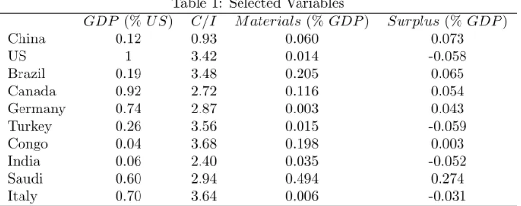
Table 1 presents, for the ten groups, values of some relevant variables. Rel-ative to the US, GDP varies across groups from 4%, for "Congo", to 92% for "Canada." There is also a large variation of mineral and hydrocarbon produc-tion as a proporproduc-tion of GDP, which ranges from 0.3% in the "Germany" group to 49.4% in the "Saudi" group, while current accounts vary from a de…cit around 6% of GDP in the US and in "Turkey," to a surplus of 27% of GDP in the case of the "Saudi" group. More relevantly, current account surplus in China stands as 7.3% of GDP.
Table 1: Selected Variables
GDP (%U S) C=I M aterials(% GDP) Surplus(%GDP)
China 0.12 0.93 0.060 0.073
US 1 3.42 0.014 -0.058
Brazil 0.19 3.48 0.205 0.065
Canada 0.92 2.72 0.116 0.054
Germany 0.74 2.87 0.003 0.043
Turkey 0.26 3.56 0.015 -0.059
Congo 0.04 3.68 0.198 0.003
India 0.06 2.40 0.035 -0.052
Saudi 0.60 2.94 0.494 0.274
Italy 0.70 3.64 0.006 -0.031
We pick the country-speci…c variables so that at the balanced growth paths corresponding to our equilibrium conditions, we match the data in Table 1.
The match is exact to the second signi…cant digit. The values ofmjandSj are
hand, we have data for the total mineral sector (energy and non-energy) for all the countries in our sample, but we have that split between the two categories only in a small subset.
used directly to match the columns for "oil" (again, minerals and hydrocarbon production as a fraction of GDP) and current account surplus. We calculated
thezj to match the PPP per capita GDP ratios, and the j to match theC=I
ratios.
5
Results
We calculate the balanced growth path for this economy given the calibration described in the previous section. That is, we obtain for each country the value of = f ; K1; K2; w; r; pc; pI; Y; c; Ig, and for the global economy the prices
p= fp1; p2g. One should notice that the calibration delivers a specialization
pattern that mimics, in a very stylized form, world specialization: Out of the 10 countries/groups, the poorest two - India and Congo - are on the balanced growth path fully specialized in the production of the labor intensive
interme-diate good (hence, = 1); China, Brazil and Turkey are diversi…ed –hence
2(0;1)– and the six remaining groups (Canada, US, Germany, Italy, Saudi
and Canada) are fully specialized in the capital intensive intermediate good, so
= 0.
We will perform several simulations to obtain the impact of certain economic phenomena. In some of these exercises, it would be interesting to distinguish between the short and the long run. Speci…cally, in each simulation exercise we assume that the economy is on the balanced growth path, and then consider the adjustment process to a new balanced growth path as we hit the economy with a one-time, permanent and unanticipated shock to some parameter. We distinguish two phases in the transition:
1. Theshort run, characterized by the new equilibrium prices, labor/oil
allo-cations and …nal outputs when we take as given not only the pre-shockK,
but also K1; K2, and allow labor and oil to ‡ow across industries
(vary-ing ), and for the prices and the c - I choice to respond to the new
parameters. These prices, and the new parameters, determine the new equilibrium allocation immediately after the shock, that is, before capital ‡ows across industries and the total capital stock start moving towards its new steady state.
2. The long run, as characterized by the new balanced growth path. We
5.1
Fracking
One of the world-changing phenomena that has emerged with increasing strength in the last few years is the use of new technologies in the extraction of hydrocar-bons (of which fracking –or hydraulic fracturing for tight oil-and-gas deposits– and the exploration of shale gas, are the best known). Because of the origin of the technology, the regulatory situation, and the kind of hydrocarbon deposits on which the new technologies perform better, these changes have been largely concentrated on the energy production of the US, that has become once again the largest producer of hydrocarbons in the world, and may become a net ex-porter in the next few years. Our …rst simulation is to …gure out the impact of the adoption of these technologies on our modelled global economy, by looking
for the short and long run e¤ects of changes in the parametermU S that match
the new production realities.
As time goes by, the increase of oil production in the US impacts prices, which then a¤ect investment and future capacity. We should be careful, thus, in the period of the data we use to …gure out how big is the impact of the new technology. For instance, if we go too far back in time to assess the changes in output, we will be capturing the e¤ects of the global recession, not just of the technology; if we go too far in the future, we would be watching the impact of prices and of recent political events in some competing producing countries. We choose for our estimates the period between 2011 and 2014, when –according to the International Energy Agency– the fracking technology innovation, which allowed the extraction of oil in areas that were not previously economically pro…table, explained most of the growth in US fossil fuel output, which was 49.35%; because there is a non-energy component of mineral production in the US, this corresponds to a change of 47% in US mineral production. By the end
of that period, the resulting and rather large fall in prices had not yet started.6
Of course, plenty of arguments can be found to argue that the shock in oil+gas supply was di¤erent than the one we assumed in our exercise. Other countries (notably Canada and Australia) are also using extensively the new technologies, let alone its eventual di¤usion to other late adapters. There are also many di¤ering sources and data for hydrocarbon supply that vary in the details. This is why we considered the robustness of our exercise to alternative
sizes in the change of mU S, and in particular describe below an alternative
experiment using an increase of 60% (the extreme among the other data sources and interpretations that we considered).
In the simulation, the main e¤ect of the increase inmU S by 47%, of course,
is a big fall in the price ofm, nearly 35.6% on impact (45.2% in the alternative
experiment where mU S increases by 60%). The model is able to explain a
large part of the short run ‡uctuation in oil prices. If we consider the average price of crude oil in 2014 as our time-0 price, the observed decrease of prices
6Non-hydraulic fracking has existed as a practical technology since the mid-1860s, and the
to March 2016 is 62%. Hence, our benchmark calibration explains 57% of this
fall.7 However, in the long run, the price fall is not as big: prices rebound
as more capital is accumulated, and more oil is demanded to satisfy increased demand for intermediate goods. The simulation results are of a long-run price
fall of only 19.7% (or 25.1% in the alterative experiment).8
Once oil is cheaper, of course, there are other secondary e¤ects across
indus-tries. In particular, the labor-intensive intermediate good1 is also much more
dependent on material than good2, and the fall in the oil prices translates in
a shift of resources towards the production of good1. The relative price of the
capital intensive good goes up by 5.7% on impact (2.6% in the long run), but
that is not enough to compensate the e¤ect of the cost of oil, so goes up in
the three groups where it can: the diversi…ed countries labelled Brazil, China and Turkey. This e¤ect is, again, stronger in the short run; a world richer in oil will use part of it to accumulate more capital, and this would bring up a countervailing shift of resources towards the capital-intensive industry in the long run. In fact, the global capital stock will end up increasing by 1.6%.
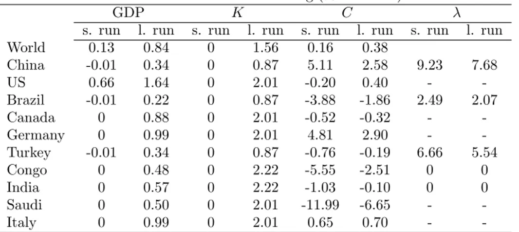
After all, due to the relatively low market share, a 47% increase in US hydrocarbon production only changes the global supply by 2.1%. The aggregate change in global output is not that large: 0.14% in the short run (when it only re‡ects the impact of a little bit extra oil), 0.85% in the long run (when it
re‡ects the new oil, and the new capital the oil allows)9. The impacts are also
comparatively small in the global levels of consumption, capital and , as shown in the …rst line of Table 2.
7Of course, to March 2016 global oil supply has also increased beyond the levels contained
in the experiment.
8We simulated the model with alternative changes in the oil supply. the short- and long-run
e¤ects change smoothly and the main results robust to alternatives.
9Note that results are in line with econometric estimations. Table 1 in Hamilton (2006)
Table 2: The E¤ects of Fracking (% variation)
GDP K C
s. run l. run s. run l. run s. run l. run s. run l. run
World 0.13 0.84 0 1.56 0.16 0.38
China -0.01 0.34 0 0.87 5.11 2.58 9.23 7.68
US 0.66 1.64 0 2.01 -0.20 0.40 -
-Brazil -0.01 0.22 0 0.87 -3.88 -1.86 2.49 2.07
Canada 0 0.88 0 2.01 -0.52 -0.32 -
-Germany 0 0.99 0 2.01 4.81 2.90 -
-Turkey -0.01 0.34 0 0.87 -0.76 -0.19 6.66 5.54
Congo 0 0.48 0 2.22 -5.55 -2.51 0 0
India 0 0.57 0 2.22 -1.03 -0.10 0 0
Saudi 0 0.50 0 2.01 -11.99 -6.65 -
-Italy 0 0.99 0 2.01 0.65 0.70 -
-But these small numbers for the world as a whole hide the more interesting aspect of the propagation: di¤erent countries are a¤ected in very di¤erent ways. Through terms of trade, and the di¤erentiated way in which the participants of trade relate to the market, the per-country e¤ects are very heterogeneous.
Take, for instance, Canada and Brazil. Both are comparatively rich in hydro-carbon endowments, and therefore a¤ected by a deterioration in their terms of trade when fracking starts elsewhere and brings prices down. Not surprisingly, both have a fall in consumption in the short run. But the impact is not exactly the same in both places. Canada has almost three times the productivity of Brazil, so they are rich in capital and fully specialized in the capital intensive
good2, while Brazil is diversi…ed. The fall in the oil price pushes up in Brazil
(a shift away from the capital-intensive good), reducing the value of capital so that the long-run change in the capital stock is just 0.87%; meanwhile, Canada
remains fully specialized in good2and the capital stock grows by 2%. Hence,
Canada fares better than Brazil (both lose in welfare - consumption - terms). The impact, on the other hand, is larger in Congo (completely specialized in the labor-intensive –and oil-intensive– good) and even larger in Saudi (stronger dependence on oil exports).
The opposite happens in countries that happen to be oil importers. Compare India, China and Germany. The …rst su¤ers a small fall in consumption, while the other two have large increases, especially in the short run. Oil dependence becomes a blessing when oil prices fall, and the stronger the dependence, the stronger the e¤ect. If, on top of that, the country is producing the oil-intensive good, the bene…ts are larger in the short run; further capital accumulation implies the opposite in the long run. Notice that China gains more from fracking immediately, but in the new steady state Germany is the biggest winner.
5.2
Consumption Increase in China
In the last three decades, a large part of the dramatic growth of the Chinese economy is owed to very fast capital accumulation. The ratio of private con-sumption to output has kept falling consistently, from about 50% in the early 1970s to about 35% in recent years. Even the former rate is low compared to the consumption levels we see in the US (between 70% and 80%) and even Germany
(60% to 70%).10
In recent years, at the outset of the Great Recession, China has started phas-ing out some of the economic features and policy choices that distort the con-sumption/investment decision towards the latter. Beyond the reasoning behind this change, we wonder here about its global, long-term implications. What are
the consequences for our model economy of an increase in the ChineseC=Iratio,
prompted by an increase in CH. A less frugal China will accumulate less
cap-ital in the long run, and therefore demand fewer materials. It will also shift production from capital-intensive to labor-intensive intermediate good. Both changes will a¤ect the world prices of tradeable goods, prompting (as before) small e¤ects on the aggregate global numbers, but large and disparate e¤ects on individual countries.
In our main scenario, we apply a change in CH from 0.436 to 0.57, which
makes the C=I ratio raise from 0.93 (the number we calibrated to), to 1.5.11
This brings about an 11% fall in oil prices, and a 3.3% increase inp2=p1. 12 In
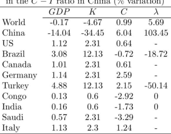
the long run, as the economy settles into a new equilibrium, the impact on the Chinese economy is, as expected, very large. The capital stock falls by 34.5%, so output falls by 4% while consumption increases by 6%. The specialization
pattern changes dramatically, since moves from 0.36 to 0.73. In fact, China
shifts from a minor importer to a large exporter of good 1.
1 0Of course, Chinese growth also owes a lot to TFP expansion –hence the next section. 1 1The reader may wonder aboutC=I= 0:93;which is not consistent with theC=Y = 0:35
fact mentioned above. Notice, however, that the latter fact relates to private consumption, while in our model we are calibrating to total consumption and total investment (since the model lacks a government).
1 2If we change
CH to a larger value such as 0.75, the fall in oil price would be around
15% andp2=p1 would increase by 5%. TheC=Iratio would be 2.24 in the long run, close to
Table 3: The Long-Run E¤ects of Changes
in theC Iratio in China (% variation)
GDP K C
World -0.17 -4.67 0.99 5.69
China -14.04 -34.45 6.04 103.45
US 1.12 2.31 0.64
-Brazil 3.08 12.13 -0.72 -18.72
Canada 1.01 2.31 0.61
-Germany 1.14 2.31 2.59
-Turkey 4.88 12.13 2.15 -50.14
Congo 0.13 0.6 -2.92 0
India 0.16 0.6 -1.73 0
Saudi 0.57 2.31 -3.29
-Italy 1.13 2.3 1.24
-The interesting part, on the other hand, is the propagation of the Chinese adjustment to the other countries. First, the vacuum left by the missing Chinese capital will be …lled in the rest of the world. Global capital stock will fall by only 4%, since there is an expansion in the steady state capital stock of all countries, and especially in the groups that happen to be diversi…ed: Brazil and Turkey.
In fact,KBRgoes up by over 12 %.
Global real GDP falls slightly by 0.17%, but all countries except China experience an increase of real GDP. The big winners are Brazil, Turkey and the US, where GDP growth in the long run is 3.1%, 4.8% and 1.1%, respectively. There is global growth in steady-state consumption, by nearly 1%, concentrated in the oil-poor or the capital-rich countries. Germany, who is both, is the biggest winner. In contrast, Brazil, Congo, India and Saudi, for either reason, are the losers.
Hence, China’s drive toward a new growth model in which the country shifts from investment to consumption will have not only sizable domestic impacts, as expect, but will a¤ect di¤erent countries in di¤erent forms. Welfare, measured as steady-state consumption, in Brazil and in similar economies will decrease, the same being true for oil rich economies, although GDP and investment will expand in all these economies.
5.3
TFP slowdown in China
Along with the hydrocarbon production technology, and the shift towards con-sumption in China, there is a third world-shaping event that is often discussed in the specialist press: the slowdown and "normalization" of the Chinese economy. In other words, the belief that China will become more similar to the rest of the world not only in its savings rate, but also in the growth rate of productivity.
roughly 0.4% annually, with a very low dispersion across groups; meanwhile, China´s TFP annual growth was 4%.
What is the impact of this Chinese "normalization"? What is the counter-factual if instead of being immediate, it took –say– 10 years for China´s TFP growth to fall gradually to global averages?
Obviously, in the long term our global economy would still converge to a balanced growth path, since after the transition period the TFP growth rates would be common across countries. But the starting point of the convergence to this new balanced growth path would not be with current TFP ratios across countries: it would be after some years of divergence.
If CH converges to average geometrically over ten years, the boost in
zCH relative to the other zj would be of 22.51%. Therefore, we compare the
steady state from our calibration with one where Chinese productivity is 22.51% higher.
The …rst thing to look at, as before, is the price of oil. In this case, higher Chinese TFP adds up to 24.7% higher price of oil in the short run, 28.7% in
the long run.13 Also, the relative pricep
2=p1 falls by 5.5%. Capital-rich and
oil-poor countries bene…t from a faster "normalization" of the Chinese economy, and vice versa.
Table 4: The E¤ects of higher steady state TFP in China (% variation)
GDP K C
s. run l. run s. run l. run s. run l. run s. run l. run
World 2.35 2.15 0 2.97 3.04 1.78 -1.84 -5.09
China 21.11 36.85 0 31.67 33.87 25.91 -9.17 -88.47
US 0 -1.99 0 -4.03 0.6 -0.33 -
-Brazil -0.01 -3.17 0 -12.27 2.69 2.97 -2.47 15.29
Canada 0 -1.79 0 -4.03 0.46 -0.24 -
-Germany 0 -2.01 0 -4.03 -3.3 -5.17 -
-Turkey -0.01 -5.01 0 -12.27 0.55 -1.3 -6.62 40.97
Congo 0 -0.53 0 -2.44 3.83 5.42 0 0
India 0 -0.64 0 -2.44 0.63 2.05 0 0
Saudi 0 -1.02 0 -4.03 8.51 9.44 -
-Italy 0 -2.01 0 -4.03 -0.38 -1.81 -
-A slower Chinese deceleration, on the other hand, would imply a capital stock higher by 31.7% in China, and this generates the price incentives for a fall in capital in the other countries. The biggest di¤erence is in the other diversi…ed countries, since the production function is linear in their relevant interval, and therefore requires larger changes in capital for a similar fall in the marginal productivity of capital. The capital stock in Brazil and Turkey would fall by 12.2%, as opposed to falls of 4% in the rich economies, and 2.4% in the poor
1 3One should be careful to understand what this means. The status quo until recently was
ones. Not surprisingly, production and real income also shift to China and to the poorer countries. World real income increases by 2.1%, and China´s by an impressive 16.3% in the short run, 28.9 in the long run. China also becomes almost specialized in the capital-intensive good, while Brazil and Turkey move in the opposite direction. Finally, welfare as measured by consumption increases in the oil-rich Saudi by an remarkable 9.4% and also in poor economies such as
India and Congo, that were bene…ted by the relative increase inp1prices. The
increase of consumption in China, as expected, was very large.
6
Conclusion
We have conducted three experiments on our calibrated model economy, re‡ect-ing three salient global events that are reshapre‡ect-ing our world: the emergence of new technologies –like fracking– for the production of hydrocarbons, and the transition of China towards its new economic model, which involves both an increase of their very low consumption-to-investment ratio, and the slowdown of their abnormally high TFP growth. All three events have in common that
they push oil prices down,14 and this propagates across the world in a
vari-ety of ways, generating an improvement in terms of trade that bene…ts the oil importers (Germany, Japan, India, etc.) and damages the energy-rich countries. Cheaper oil has as a second consequence that resources shift in the short run towards the labor intensive good (because it is also oil-intensive), and in the long run in the other direction (because more oil allows for more capital accumulation). Again, this has di¤erent e¤ects on capital-rich and capital poor countries.
Conceptually, we …nd the main contribution of this work to be in the possibil-ity to analyze how global events propagate di¤erently among di¤erent countries, through trade channels that a¤ect each participant depending on its features and comparative advantage. In several of the experiments conducted, we ob-serve capital or consumption react in one direction for some countries and the opposite for others. Most macro models of the international economy would not capture this subtlety, since countries relate to each other via income channels, and every event moves everybody in the same direction. In fact in our model, quantitatively the aggregate e¤ects of these events globally are not very large, compared to the individual e¤ects in di¤erent economies. For example, the im-pact of our fracking experiment changes global consumption by 0.4% only, but this hides increases of as much 3% in "Germany" and falls of as much as 6.7% in "Saudi".
These results are robust to di¤erent compositions of groups, calibration and, qualitatively, to the magnitude of shocks. We could also have reproduced the
1 4In the …rst and second experiments, oil prices fall in the short run, and bounce partially
experiment for the 176 individuals countries we have data. The main message of the paper would be the same: if China’s new model of development and the increase in oil supply are permanent phenomena, which seem to be the case, we are about to observe important distributional e¤ects of world output across countries and, maybe more importantly, of welfare.
References
[1] Acemoglu, D. and V. Guerrieri (2008) "Capital Deepening and
Nonbal-anced Economic Growth," Journal of Political Economy, vol. 116(3),
467-498.
[2] Atkeson, A. and P. J. Kehoe (1999), “Models of Energy Use: Putty-Putty Versus Putty-Clay,” American Economic Review, 89, 1028-1043.
[3] Bajona, C. and T. Kehoe, (2010) "Trade, Growth and Convergence in a Dynamic Heckscher-Ohlin model", Review of Economic Dynamics, 13(3), 487-513.
[4] Beaudry, P. and F. Collard (2006) "Globalization, Returns to Accumulation and the World Distribution of Output", Journal of Monetary Economics, 53(5), 879-909.
[5] Bond, E., Iwasa K, and K. Nishimura , (2011). "A Dynamic Two Coun-try Heckscher-Ohlin Model with Non-Homothetic Preferences", Economic Theory, 48(1): 171-204.
[6] Brandt, L., Tombe,T and X. Zhu, 2013. "Factor Market Distortions Across Time, Space, and Sectors in China," Review of Economic Dynamics, vol. 16(1), 39-58.
[7] Corden, W. (1971), "The e¤ects of trade on the rate of growth", in
Bhag-wati, Jones, Mundell and Vanek,Trade, Balance of Payments and Growth,
(North-Holland), 117-143.
[8] Deardor¤, A. (2001), "Rich and Poor Countries in Neoclassical Trade and
Growth,"The Economic Journal, 111(April), 277-294.
[9] Dekle, R. and V. Guillaume, (2012). "A Quantitative Analysis of China’s Structural Transformation," Journal of Economic Dynamics and Control, 36(1), 119-135.
[10] Ferreira, P. C. and A. Trejos (2006), “On the Long-run E¤ects of Barriers
to Trade,”International Economic Review, 47(4), 1319-1340.
[12] Hamilton, J. D. (1983), “Oil and the Macroeconomy Since World War II,” Journal of Political Economy, 91, 228-248.
[13] Hamilton, J. D. (1988), “A Neoclassical Model of Unemployment and the Business Cycle,” Journal of Political Economy, 96, 593-617.
[14] Hamilton, J. D. (2003), “What is an Oil Shock?” Journal of Econometrics, 113, 363-398.
[15] Hamilton, J. D. (2008), "Oil and the Macroeconomy," in New Palgrave Dic-tionary of Economics, 2nd edition, ed. Durlauf, S. and L. Blume, Palgrave McMillan Ltd.
[16] Kim, I. and P. Loungani (1992), “The Role of Energy in Real Business Cycle Models,” Journal of Monetary Economics, 29(2), 173-189.
[17] Rotemberg, J., and M. Woodford (1996), “Imperfect Competition and the E¤ects of Energy Price Increases,” Journal of Money, Credit, and Banking, 28 (part 1), 549-577.
[18] Song, Z., Storesletten, K and F. Zilibotti (2011), "Growing Like China," American Economic Review, 101(1), 196-233.
7
Appendix
From (6) we can derive the …rst order conditions
wj = (1 i)(pi i)zLij iKiji
rj = (pi i)zL1ij iK i
1
ij ;8i= 1;2; j = 1; :::;
Equating wages and rents across industries, and applying (10), delivers as an interior solution
e
k1 =
"
2 1
2 1
2
1 1
1 2p
2 2
p1 1
# 1 1 2
(15)
e
k2 =
"
2 1
1 1
2
1 1
1 1p
2 2
p1 1
# 1 1 2
e = 1(1 2)k 2(1 1)ek1 ( 1 2)ek1
It follows that ek1 < k <ek2 if and only if e2[0;1]. Then the economy will
be diversi…ed among the intermediate goods so =e, k1 =ek1 and k2 = ek2.
However, if the economy is so capital abundant thatek2< k, then = 0,k2=k;
similarly, if it is so labor abundant thatek1> k then it specializes in producing
independent of k if the economy is diversi…ed: the Factor Price Equalization Theorem of the Hecksher-Ohlin model. Substituting (15) in (1) and (2) one can
obtainQ1; Q2, and from
X(k) = (p1 1)Q1+ (p2 2)Q2+m S
one obtains (13). Alternatively, one can derive the same result from X(k) =
w+rk+m S.
To derive consumption and investment, derive from the FOC of (7) that
q2c
q1c =
1 p1
p2 (16)
q2i
q1i
= 1 p1
p2
Along with (8) this transforms into
pc =
p1p12
zc (1 )1
(17)
pi =
p1p12
zi (1 )1
and one can derive thenqic; qiI as functions ofI; cfrom (3), (16) and (17).
I = ( k)1=
c = X(k) pi( k)
1=
pc
To obtain I; c and close the model, construct the dynamic programming
problem
V(k) = maxu(c) + V(k0) s:t:
X(k) = (1 + )pcc+ piI
k0 = (1 )k+I
This Belman equation can be expressed unconstrained as
V(k) = maxu
"
X(k) pi[k0 (1 )k]1=
(1 + )pc
#
+ V(k0) The Envelope Theorem then amounts to
V0(k) = u0(c)
(1 + )pc
h
X0(k) + (1 )p
i[k0 (1 )k]
1= 1
which combined with the …rst order condition
u0(c)
(1 + )pc
pi[k0 (1 )k]1= 1= = V0(k0); transforms in steady state into
[1 (1 )]pi[ ]1= 1
=X0(k)k( 1)= ;
which is exactly (14), the critical Euler equation for this problem. Notice that
<1 is what allows this system to have a unique solution, since X is weakly