A REGULARIZED GMRES METHOD FOR INVERSE
BLACKBODY RADIATION PROBLEM
by
Jieer WUaand Zheshu MAb*
aSchool of Mathematics and Physics, Jiangsu University of Science and Technology, Zhenjiang, China
bDepartment of Power Engineering, Jiangsu University of Science and Technology, Zhenjiang, China
Original scientific paper DOI: 10.2298/TSCI110316078W
The inverse blackbody radiation problem is focused on determining temperature distribution of a blackbody from measured total radiated power spectrum. This problem consists of solving a first kind of Fredholm integral equation and many nu-merical methods have been proposed. In this paper, a regularized generalized mini-mal residual method is presented to solve the linear ill-posed problem caused by the discretization of such an integral equation. This method projects the original prob-lem onto a lower dimensional subspaces by the Arnoldi process. Tikhonov regular-ization combined with the generalized cros validation criterion is applied to stabi-lize the numerical iteration process. Three numerical examples indicate the effectiveness of the regularized generalized minimal residual method.
Key words: blackbody radiation, inverse problem, generalized minimal residual method, regularization
Introduction
During theoretical study of blackbody radiation problems, we often use a set of inaccu-rate experimental data to calculate other physical data. The inverse blackbody radiation (BRI) problem is one of the examples. According to Planck's law, the mathematical model of the blackbody radiation can be expressed as [1]:
w v hv
c
a T T
hv/kT
( )= ( )
-ò
2
1 3
2 0e
d 4
(1)
where frequencyvÎ[V1,V2],w(v) is the total radiated power spectrum,T– the absolute temper-ature and the range ofTusually goes from 100 to 1000 K,a(T) – the area temperature distribu-tion,c– the speed of light,k– the Boltzmann's constant, andh– the Planck's constant. The direct problem of blackbody radiation is to calculatew(v) bya(T) while the BRI problem is to obtain
a(T) by solving in integral eq. (1). The BRI problem is important in remote sensing applications. For convenience lettingG(n) =c2w(v)/2hv3and then expression (1) is equivalent to:
G( ) a T( ) T K v T a T( , ) ( ) T /
n
n
=
- =
ò
e dò
dh kT 1
0 0
4 4
(2)
where integral kernelK(n,T) = (ehv/kT– 1)–1. Equation (2) is a first kind of Fredholm integral equation and is an inherently ill-posed problem [1]. Since 1982, this problem has attracted many
scholars' attention. The first formulation for this problem was proposed by Bojarski [2] in 1982. The Laplace transform together with an iterative process was presented. Chen and Li [3], Dai and Dai [4] proved the existence and uniqueness of the solution of BRI. Sun and Jaggard [5], Dou and Hodgson [6], and Li and Xiao [7] discussed Tikhonov regularization methods. Li [8] proposed conjugate gradient method. Dou and Hodgson [9] employed maximum entropy method. Yeet al. [10] developed universal function set method. Wu and Dai [11] presented a regularizing Lanczos method.
Generalized minimal residual (GMRES) algorithm method [12] is a common tool for solving linear systems. Until recently GMRES method has been applied to discrete ill-posed problems. For instance Jensen and Hansen [13] systematically studied the characteristics of the regularization GMRES method. Calvettiet et al. [14, 15] discussed regularization GMRES method and applied theLcurve condition number to solve linear ill-posed problems and image restoration processing. In this paper, we discrete the integral eq. (2) and introduce the GMRES method to solve the obtained linear discrete ill-posed system. This method is based on the Arnoldi process, which yields a sequence of small least squares problems by approximating the original discrete ill-posed problem. Tikhonov regularization [1] combined with generalized cross validation (GCV) criterion [16] are used to stabilize the iteration process. Numerical re-sults illustrate the potential of the proposed method.
Discretization and regularization
In practice, the range ofTusually goes from 100 K to 1000 K, andvgoes from 0 Hz to 2×10¹⁴Hz. Assuming the range ofTis [T
1,T2], then eq. (2) can be expressed approximately as:
G v a T T
hv/kT T T
( )= ( )
-ò
e 1d
1 2
(3)
LetnÎ[V1,V2], we choosencollocation points:v1=V1+l(V2–V1)/(n– 1),l= 0, 1,...n– 1 on the [V1,V2], then eq. (3) becomes:
G vl a T T l n
hv kT j
n
l
( ) ( ) , , , ...,
/
=
- =
-=
-ò
e d1 0 1 1
0 1
(4)
The numerical quadrature ruler f x x b a f a
a b
( )d »( ) ( )
ò - withnintervals of equal length
on [T1,T2] is discreted as:
G a T T T T
n
a t
l hv kT
t t
j n
j hv
l j j
( ) ( ) ( )
/
n =
-ò =
-+
=
-å
e 1d e
1
0 1
2 1
l ktj
j n
/
-=
-å
1 0
1
(5)
If the vectorsxandbare defined byx= [a(t0), ...,a(tn–1)]T,b= [G(v
0), ...,G(vn–1)]T, and if then´nsquare matrix [A] is defined byA= (d/ehvl/ktj– 1)
n·nwhered= (T2–T1)/nthen eq. (5) can be written as:
Ax=b (6)
One of the most common methods of regularization is Tikhonov regularization [1], which replaces the system (6) by the minimization problem
x
min Ax b- 2 +l2 x 2or equiva-lently:
(ATA+l2I)x=ATb (7)
where l2 is a regularization parameter and ||×|| denotes the 2-matrix norm. Combining the GMRES method with Tikhonov regularization [1], system (6) is projected onto a Krylov subspace. The projected problem is also ill-posed. Since the dimension of the projected problem is usually small relative ton, regularization of the projected problem is much less expensive.
Regularized GMRES method
The GMRES method which based on the Arnoldi process is a popular iterative method for solving large linear system with a non-symmetrical non-singular matrix. In exact arithmetic, for a given starting vectorr0, the GMRES method projects system (6) to Krylov subspace:
Km(A,r0) = span{r0,Ar0, ...Am–1r
0} and determines iteratesxmÎx0+Km(A,r0),m= 1, 2, ...,
which satisfy: b Axm b Ax
x Km A b
- =
-Îmin( , ) . We use notation (x,y) =xTy,x,y
ÎRNin the following Arnoldi process.
Algorithm 1. (The Arnoldi process)
(1) letx0be a starting vector. Computer0=b–Ax0andv1=r0/||r0||; (2) forj= 1, ...,m; (2.1) com-puteh=Avj; (2.2) fori= 1, ...,jcomputehij= (h, vi) andh=h–hijvi, (2.3) computehj+1,j= ||h||, and (2.4) computevj+1=h/hj+1,j.
The Arnoldi process generates an orthonormal matrixVm+1= [v1,v2, ...,vm+1] whose columns are orthonormal bases of Km(A,r0), and an upper Hessenberg matrix Hm=(hij)Î ÎRm,m–1. In matrix form we have:
AVm=V Hm m +hm m mv eT
+1, +1 1 (8)
wheree1is the first canonical vector.
Let ~
,
H H
v e
m m
m m m T
h
=æ è ç ç
ö
ø ÷ ÷
+1 +1 1 ,
the GMRES method computes the approximation xm= x0 + Vmy, where y solves the least squares problem:
b-Ax = b-A x +V y = r e -H y
Î Î
m
y Rminm ( m y Rminm m
~
0 0 1 (9)
Generally with the increasing iteration, the largest and the smallest singular value of matrixH~mwill approximate those of matrixA, respectively. This means that the problem (9) in-herits properties of the system (6) and is also a small ill-posed problem. Therefore we use Tikhonov regularization method to regularize (9) and solve:
(H H~mT ~m +l2I y) = r0 H e~mT 1 (10) Suppose that the singular value decomposition (SVD) ofH~mis given by:
~
Hm =Pæ Q è çç ö
ø ÷÷
W
0
T (11)
y= r P q + =
å
0 2 2 2 1 1 ww l w i i i i i m i (12)
There exists different ways of choosing the regularization parameter. Here the GCV criterion is employed. This method is to find the parameterlthat minimizes the GCV function:
G( ) ( )
[ )]
#
l l
l
= I-HH r e I – HH#
0 1 2
2 tr(
whereHl# =(HHl# +l2I)–1HT. Here the symbol HisH~
min eq. (8) and tr(A) denotes the trace ofA.
Proposition 1. DenoteKi=l2/(w
i
2 +l2),i= 1, 2, ...,m, then:
G
K
m K
i i m
i m i m ( ) ( ) l = + å é ëê ù ûú + - å
+ =
=
r0 2 P1 2 P
12 1 1
1 1 1
(13)
Proof. Following eq. (11) it is immediate to see that:
I-HH =PéI - + I P
ë ê ù û ú l l # – ( )
m W W T
2 2 2 1
1
0
0
Since tr(AB) = tr(BA), we have:
tr( #) tr ( )
–
I-HH = éI - + I ë
ê ù
û
ú = + - å=
l l m i i m m K
W W2 2 2 1
1
1 1
0
0
Moreover, the numerator is:
( # ( ) (
–
I -HH r e = r éI - + I P e r P
ë ê ù û ú = l l
0 1 0
2 2 2 1
1 2 0 1 m T i K W W 0 0 1 1 2
12 1
i i m m = + å + é ëê ù ûú ) P
thus eq. (13) holds generally.
The proposition 1 suggests that one can estimate parameterlby finding the minimum value of eq. (13). Iflis known, then the approximate solutionxm=x0+Vmycan be found by eq. (12). The algorithm 2 summarizes how the computations for the regularized GMRES can be or-ganized.
Algorithm 2.(Regularized GMRES method)
(1) compute the linear system (6) by discretizing eq. (3), (2) choose a starting vectorx0and carry outmsteps of the Arnoldi process, (3) compute the SVD ofH~m, (4) solve eq. (10) using GCV criterion, (5) setxm=x0+Vmyk, and (6) check convergence. If not converged letm=m+ 1 and continue iterating.
In the algorithm, the iteration numbermshould not be too large. Usually we can set an upper limit for the number of iteration m. If the Krylov subspace dimension increases up to the maximum iteration number and the residual norm ||b–Axm|| is not small enough, we can apply the restarted GMRES method to get the iteratexm.
Numerical results
For numerical error estimation, we define the relative er-ror as:g= ||a(T) –xm||2/||a(T)||2, wherea(T) is the exact temper-ature distribution andxm– the approximate solution calculated by the regularized GMRES method.
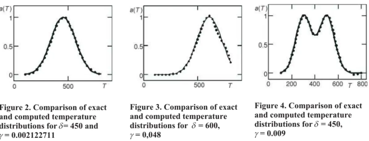
Example 1 is a Gaussian temperature distribution given by:a(T) = exp[–(T–d)2/25000],TÎ[100, 800], wheredis a parameter. For a givenn= 50, we discrete (3) and obtain the linear system (6). It is easy to know that the coefficient matrix Awithd= 450 is ill-conditioned because the largest singular value of matrixAis 5.153·104and the smallest singular value is 0. Letd= 200, 450, and 600. Application of the regularized GMRES method to these distributions results the temperature distributiona(T) as shown in fig. 1-3. These figures display the comparisons of the approximate solution determined by
the regularized GMRES method indicated by the dotted curve and the exact solution (solid curve). Obviously the overall agreement between calculated and exact values displayed in fig. 1 and fig. 2 is excellent. For the case of d= 600 the resulted distribution shown in fig. 3 has some disagreement and the corresponding relative errorg= = 0.048. This result is good and can be acceptable.
Example 2 is the double Gaussian temperature distribution given by:a(T) = exp(T– – 300)2/9000 + exp(T– 600)2/9000,TÎ[100, 800].
The computed results in fig. 4 shows good, but the cal-culated distributionsa(T) indicated by the dotted curve have some disagreement at the right part.
Example 3 is that of a rectangular temperature case:
a T T
T
T
T
( )
.
. ,
= -
-£ < £ < £ <£
ì 05
1 450
300 05
100 300
300 600
600 00
í ïï
î ï ï
In this example the distributionsa(T) is continuous, but not differential at some collocation points. Figure 5 shows the
Figure 1. Comparison of exact and computed temperature distributions ford= 200 and g= 0.000113216
Figure 2. Comparison of exact and computed temperature distributions ford= 450 and g= 0.002122711
Figure 3. Comparison of exact and computed temperature distributions for d= 600, g= 0,048
Figure 4. Comparison of exact and computed temperature distributions ford= 450, g= 0.009
calculated result (dotted curve) for this example. The agreement in the part of lower temperature is satisfactory but the oscillations appear in the right region. This phenomenon indicates that the discontinuity and the intrinsic instability of the physical problem effect the reconstructed result.
Conclusions
In this paper the regularized GMRES method is introduced to recover thea(T) from the total power spectral measurements of its radiation. From the limited numerical results we find that the proposed algorithm is numerically stable and can recover thea(T) which is continually differen-tial.
References
[1] Tikhonov, A. N., Arsenin, U. Y.,Solutions of Ill-Posed Problems, John Wiley and Sons, New York, USA, 1977
[2] Bojarski, N. N., Inverse Black Body Radiation,IEEE Trans. Antennas and Propagation, 30(1982), 4, pp. 778-780
[3] Chen, N., Li, G., Theoretical Investigation on the Inverse Black Body Radiation Problem,IEEE Trans. An-tennas and Propagation, 38(1990), 8, pp. 1287-1290
[4] Dai, Xi., Dai, J., On Unique Existence Theorem and Exact Solution Formula af the Inverse Black-Body Radiation Problem,IEEE Trans. Antennas and Propagation, 40(1992), 3, pp. 257-260
[5] Sun, X., Jaggard, D. L., The Inverse Blackbody Radiation Problem: A Regularization Solution,J. Appl. Phys., 62(1987), 11, pp. 4382-4386
[6] Dou, L., Hodgson, R. J. W., Application of the Regularization Methods to the Inverse Black Body Radia-tion Problem,IEEE Trans. Antennas and Propagation, 40(1992), 10, pp. 1249-1253
[7] Li, C., Xiao., T., The Fast and Stable Algorithms for the Numerical Inversion of Black Body Radiation, Chinese Journal of Computational Physics, 19(2002), 2, pp. 121-126
[8] Li, H. Y., Solution of Inverse Blackbody Radiation Problem with Conjugate Gradient Method, IEEE Trans. Antennas and Propagation, 53(2005), 5, pp. 1840-1842
[9] Dou, L., Hodgson, R. J. W., Maximum Entropy Method in Inverse Black Body Radiation Problem,J. Appl. Phys, 71(1992), 7, pp. 3159-3163
[10] Ye, J., The Black-Body Radiation Inversion Problem, Its Instability and a New Universal Function Set Method,Physics Letters A, 348(2006), 3-6, pp. 141-146
[11] Wu, J., Dai, H., Regularizing Lanczos Method for Inverse BIack Body Radiation Problem,Journal of Nanjing University of Aeronautics & Astronautics, 39(2007), 2, pp. 267-272
[12] Saad, Y., Schultz, M., GMRES: A Generalized Minimal Residual Algorithm for Solving Nonsymmetric Linear Systems,SIAM J. Sci. Statist. Comput., 7(1986), 3, pp. 856-869
[13] Jensen, T. K., Hansen, P. C., Iterative Regularization with Minimum-Residual Methods,BIT Numerical Mathematics, 47(2007), 1, pp. 103-120
[14] Calvetti, D.,et al., On the Regularizing Properties of the GMRES Method,Numerische Mathematik, 91 (2002), 4, pp. 605-625
[15] Calvetti, D.,et al., LMRES,L-Curves and Discrete Ill-Posed Problems,BIT, 42(2002), 1, pp. 44-65 [16] Golub, G. H.,et al., Generalized Cross-Validation as a Method for Choosing a Good Ridge Parameter,
Technometrics, 21(1979), 2, pp. 215-223