Universidade Federal de Uberlˆ
andia
Faculdade de Engenharia El´etrica
Programa de P´
os-Gradua¸c˜
ao em Engenharia El´etrica
The implementation of a theorem prover in
functional language and the use of the Rasch
Model combined with Condorcet-List
Theorem
Junia Magalh˜
aes Rocha
Universidade Federal de Uberlˆ
andia
Faculdade de Engenharia El´etrica
The implementation of a theorem prover in
functional language and the use of the Rasch
Model combined with Condorcet-List
Theorem
Tese apresentada por Junia Magalh˜aes Rocha `a Universidade Federal de Uberlˆandia (UFU) como parte dos requisitos para obten¸c˜ao do t´ıtulo de doutor.
Banca Examinadora:
————————————————————— Luciano Vieira Lima, Dr. UFU. Orientador (UFU) ————————————————————— Marcelo Rodrigues Sousa, Dr. (UFU)
Dados Internacionais de Catalogação na Publicação (CIP) Sistema de Bibliotecas da UFU, MG, Brasil.
R672i 2015
Rocha, Júnia Magalhães, 1985-
The implementation of a theorem prover in functional language and the use of the Rasch Model combined with Condorcet-List Theorem / Júnia Magalhães Rocha. - 2015.
122 f. : il.
Orientador: Luciano Vieira Lima.
Tese (doutorado) - Universidade Federal de Uberlândia, Programa de Pós-Graduação em Engenharia Elétrica.
Inclui bibliografia.
1. Engenharia Elétrica - Teses. 2. Inteligência artificial - Teses. 3. Processamento de linguagem natural (Computação) - Teses. 4. Prolog (Linguagem de programação de computador) - Teses. I. Lima, Luciano Vieira, 1960-. II. Universidade Federal de Uberlândia. Programa de Pós-Graduação em Engenharia Elétrica. III. Título.
The implementation of a theorem prover in functional language and the
use of the Rasch Model combined with Condorcet-List Theorem
Junia Magalh˜aes Rocha
Tese apresentada por Junia Magalh˜aes Rocha `a Universidade Federal de Uberlˆandia (UFU) como parte dos requisitos para obten¸c˜ao do t´ıtulo de doutor.
—————————————————– ——————————————
Luciano Vieira Lima, Dr. Alexandre Cardoso, Dr
Orientador Coordenador do
Agradecimentos
Em primeiro lugar agrade¸co a Deus pela for¸ca que me concedeu para a realiza¸c˜ao desse doutorado. Aos meus pais, Jos´e Antˆonio e Maria das Gra¸cas, minha irm˜a Juliane, minha av´o Nini e ao meu esposo F´abio pelo apoio incondicional. Agrade¸co a minha fam´ılia pela compreens˜ao nos momentos que estive ausente.
Aos professores Luciano Lima e Eduardo Costa pelo gigantesco conhecimento ao longo desses anos de Mestrado e Doutorado.
Aos meus amigos Rubens Barbosa e Will Roger que tanto me apoiaram nos trabalho do laborat´orio.
Contents
List of Figures . . . vi
1 Introduction 2 1.1 Objective . . . 5
1.2 Work Layout . . . 5
2 Condorcet-List Theorem and Rasch Method 7 2.1 The Jury Theorem . . . 7
2.2 Rasch Model . . . 10
2.3 Scales . . . 10
2.4 Specific objectivity . . . 12
2.5 Origin . . . 13
2.6 Rasch Logistic Distribution . . . 15
2.7 Calibration Algorithm . . . 18
3 Lisp and Mathematics 24 3.1 Tool for natural language processing . . . 27
3.2 Emacs . . . 28
3.3 Quicklisp . . . 30
3.4 Emacs commands . . . 34
3.5 Arithmetic operations . . . 35
3.6 The let-form . . . 37
3.7 Lists . . . 38
3.8 Packages . . . 41
3.10 format . . . 43
3.11 Loops . . . 44
4 An space efficient implementation of WAM 46 4.1 Concepts . . . 52
4.2 Enunciate the thesis . . . 52
4.3 Performing Tests . . . 53
4.4 Warren Abstract Machine - WAM . . . 55
4.4.1 Registers . . . 56
4.4.2 Unification . . . 58
4.4.3 The Cut . . . 59
4.4.4 Deterministic Predicates . . . 59
4.4.5 Infix Syntax . . . 60
4.4.6 Consult function . . . 63
4.4.7 Generated Lisp code . . . 63
4.5 Tests performed with WAM . . . 64
5 Future Work 78 5.1 Web pollution . . . 78
5.1.1 Text mining . . . 80
6 Conclusion 82
List of Figures
2.1 Condorcet’s Jury Probabilities . . . 8
2.2 Hit probability of the jury . . . 9
2.3 C x V . . . 11
2.4 Success and failure probabilities for problem R . . . 11
2.5 Specific Objectivity . . . 12
2.6 Origin of the Ability Scale . . . 16
Abstract
This thesis proposes the implementation of a theorem prover using a functional program-ing language. The implementation was based on the Warren Abstract Machine (WAM). The objective behind implementing the WAM is to achieve robustness and while running remain constant in both time and space. The inference engine was implemented using Common Lisp, due to its mathematical roots. The Theorem prover syntax approaches that of the language Prolog. Besides the theorem prover, it was demonstrated that the Rasch Model and the Condorcet-List can be brought together and used for the processing of natural language.
Keyword
Chapter 1
Introduction
Natural language processing (nlp) is a complex task, due to the fact that it requires analyzing underlying relationships, grammatical rules, meanings, logic and shared expe-riences.
One finds multiple meanings frequently among individual words and sentences. Besides this, one can express a concept in many different forms. Therefore, handling the ambiguity that arises from these two aspects of language poses a significant challenge to linguists.
It is a well known fact that people resolve ambiguity through the surroundig text, knowledge of the world and shared experience.
Surrounding text: Compared to other issues involving natural language processing, it is relatively simple task to analyse the surrounding text automatically.
Knowledge about the world: Procedural semantics can gather knowledge about the world.
Shared experience: The implementation of surrounding text analysis, and of a system that gathers knowledge about the world, leaves the question: How can a machine share experience with a human being? Before trying to answer such a question, let us see what procedural semantics pertain.
Procedural semantics contrasts with logical semantics, where it is assumed that facts are available in a database. In this case, the listener must match queries against this database. Critics of logic semantics claim that there is a very large amount of infor-mation that a speaker of a language must gather about the world and so the data base management system will never reach a complete set of facts. For instance, to speak at the level of a four year old child, a computer needs to know a lot of things about water alone: it freezes, it takes the shape of a glass, it boils, one can use it to take a bath, etc. People do not consult a database to obtain information about water. It is retrieved directly from observations about the world, and stored persistently in human memory. Therefore, the key is data persistence.
Instead of gathering facts about the world, procedural semantics actively constraints which facts are collected from the environment or from an interlocutor.
In order to create a model of the world and of its interaction with human beings and other machines, the computer must build a model of various objects. Of course, object oriented programming can be the basis for building a representation of the world.
Objects have attributes, like color, size, position, weight, integrity, etc. Attributes have values. For instance, colors can be white, blue, red, etc. A set of values for the attributes determines a state for an object.
Of course, objects belong to classes: birds, cities, stars, chemical elements, furniture, employers, etc. There are actions that can be performed by a system of classes. For instance, to kill is an action that can be realized by almost any kind of object. However, the consequence of killing can fall only upon animals, microorganisms or plants. Fighting requires two animals. Any act that one can perform on a set of objects is called a method. Choosing a method that will be applied to a set of objects is called dispatch.
Of course there are many methods that the computer can apply to a given set of objects. The computer can choose one of these methods or more than one. When the computer applies methods one after the other, each method adds constraints to the solu-tion. In the end, it is necessary to put together the result of the many applicable methods. This operation is called method combination, and builds an effective method.
Then, the computer sorts the list of applicable methods by placing the more specific method in front of the more general method. Finally, the machine takes the methods in the same order as found in the sorted list, and combines their code to produce the effective method. Of course there are many strategies for combining methods.
One cannot leave out the point that many computer languages that claim to be ob-ject oriented are in fact not. They fail in the first feature of obob-ject orientation: they do not have multiple dispatch. In consequence, there is no automatic method combina-tion. The programmer must hardwire the effective method inside each class. This makes implementing procedural semantics very difficult towards the impossible.
It is useless to have shared an experience with somebody else if one does not remember it. People build a common context with other people because they remember facts, events, and actions. They remember solutions to problems and the procedures for arriving at those solutions. They learn and store what they have learned as skills and behaviors. Two words sums up the building of shared experience: persistence and memoization.
Persistence refers to a state that outlives the process that created it. Without this capability, the state is lost at a computer shutdown. Let us consider a computer C that is helping a child K to write a prose composition. The computer has many methods for detecting errors and to produce appropriate advice and assessment. When a teacher corrects a mistake made by K, the computer can add a new method or constraint to the object concerned, or generate states to existing objects. However, when K turns off C, all states are lost. The common experience that C and K had together remains only in K’s memory. Of course one can add a logic rule in the C database, but this is tantamount to building a logic semantic. In the case of C and K, the child will remember his experience with the computer and teacher, but the computer will be left with a dead database.
Memoization stores the results of expensive function calls and returns the cache when the same inputs occur again. In few words, what persistence does for object states, memo-ization does for procedures and algorithms. In natural language processing, memomemo-ization is specially useful to accomodate ambiguity and left recursion in polynomial time and space.
The author believes that it is impossible to build a complex natural language processing application without targeted contributions of thousand of programmers during decades.
1.1
Objective
1. Objective 1: Implement a theorem prover based on Warren Abstract Machine. It is necessary to use a computer language that can accomodate any new technological advance, such as parallelism, persistence, memoization, etc. Its syntax and seman-tics must be based on mathemaseman-tics, so it will not suffer any substantial change from one decade to another. Finally, it must have a powerful scheme of encapsulation to prevent the work of a contributer having deleterious effects on the efforts of another researcher. The only language with all these attributes is Common Lisp.
2. Objective 2: The syntax of the proposed inference engine should be as close as possible to the tradicional syntax of Prolog.
3. Objective 3: The interface should accept declarations of deterministic predicates as well as non-deterministic predicates.
4. Objective 4: The inference engine should optimize the use of time and space. 5. Objective 5: It is also necessary to create a repository management system so that
a researcher can have instant access to all previous work. The technology for such a repository also exists, and it is called quicklisp. Therefore, the project presented herein will be available in quicklisp.
1.2
Work Layout
This study is divided into seven chapters. Chapter 1 presents an introduction to natu-ral language processing, the incumbent difficulties encountered carrying out this process become the essence of the presented thesis.
Chapter 3 functions as a foundation for understanding the programming of the codes presented in this thesis.
Chapter 4 provides details of the efficienty implementation of the Warren Abstract Machine (WAM) as proposed in this thesis.
Chapter 5 discusses the difficulties one finds when searching for information on web, this difficulty presents itself through the excessive content available. also discussions based on textmining techniques are used in order to facilitate the extraction of such information.
The conclusion for this thesis is presentes in chapter 6.
Chapter 2
Condorcet-List Theorem and Rasch
Method
The first motivating problem of this thesis was to apply Condorcet-List Theorem in a panel of experts. Deeper into the theme, the necessity of knowing the probability of success of each specialist who participated in the panel arose. At this moment, the second motivating problem emerged. How to discover the probability of success of each specialist? Would there be a measurement to each skill? Would there be a measurement for knowledge? Studying Theory of Measurement, we ascertained that the Model proposed by Rasch, Lord and Lazarsfeld may be applied to this problem.
This chapter aims at presenting how the Model of Rasch combined with Condorcet-list Theorem may be applied. The content of this chapter may be applied in several areas, such as data processing and engineering and in the problem that will be presented in the chapter 5 of this thesis, the process through which voting functions as a decantation filter, or be it produces through the majority vote a sufficient filter for finding the best content.
2.1
The Jury Theorem
Figure 2.2: Hit probability of the jury
himself, since his proof assumes that all jury members have the same hitting probability. However, Christian List and Robert Godin generalized the Condorcet’s theorem to many voters with different probabilities. Basically, they proved two propositions:
Proposition 1. There are k options, and each referee has independent probabilities
p1, p2, p3. . . pk of choosing options 1,2, ..., k. Besides this, the probability pi of
vot-ing for the correct outcome i exceeds each of the probabilities pj of voting for any
of the wrong outcomes, j 6= i. In this case, the correct option is more likely than any other option to be the plurality winner.
Proposition 2. As the number of voters/jurors tends to infinity, the probability of the correct option being the plurality winner converges to 1.
The reader will find the proof of these two propositions in [20].
In the present work the author will show how the Rasch model can be used to measure the value of a random variable, and assign a probability to the random variable that corresponds to a given measurement. In particular, the work describes how one can use the Rasch model in the identification of the information contents. Wright and Mok [21] provides a good tutorial on the Rasch model.
example of a classifier. Learning machines achieve classification goals through Artificial Intelligence schemes, like neural networks, deep learning, energy based learning, symbolic computation and genetic programming.
The author of the present work have suggested taggers coupled with the Condorcet-List theorem, Rasch method to solve the inverse problem of determining the grammatical classes of words, necessary to designing a natural language processing system. Since other researchers have placed a great number of well tested classifiers in libraries (for example, the rasp3os system) easily available to any engineer with access to the Internet and a working knowledge of Lisp, this work will concentrate on the Rasch method and the Condorcet-List theorem.
2.2
Rasch Model
In a measurement, there is a variable that one wants to evaluate. Variables like weight, temperature or height can be measured directly with scales, measuring tapes, etc. Un-observable variables like skill, efficiency, initiative, or soil electric properties are not so easy to measure. One can describe such latent variables, but cannot compare them to a standard meter, since they lack physical dimensions. However, one needs to assess them to appraise the quality of health care services, to design a grounding system or students in a particular subject.
In order to estimate the value of a latent variable, Rasch, Lord and Lazarsfeld devel-oped independently a branch of statiscs known as Measurement Theory.
Since the Rasch model proved so useful in measuring latent traits and attributes in human sciences, the author of this work used this Model for example to evaluate the grammatical classes of English words.
2.3
Scales
as being individuals.
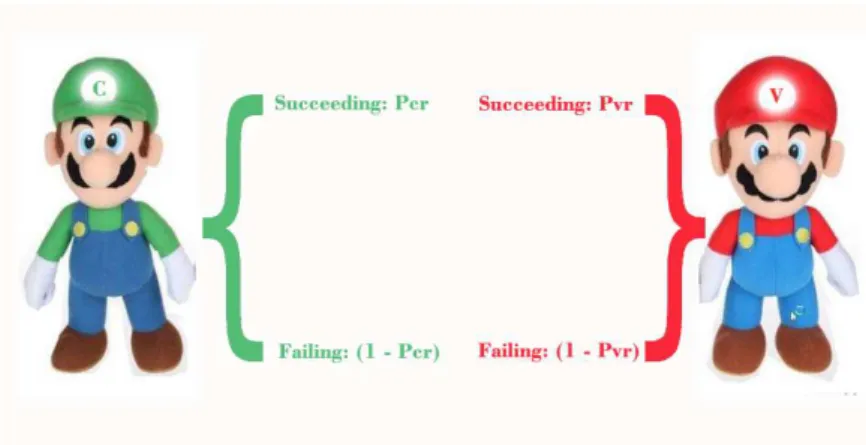
Let us consider two persons c and v, and an item r that one wants to classify. What is the probability of c hitting item r? What is the probability of v hitting item r? The first problem is to compare the skills of c and v based on their performance in resolving itemr. In this context, an item is a member of an object class. The two persons need to classify many items to arrive at a raw score.
Figure 2.3: C x V
The difference between raw scores is not a good basis for comparison. If both scores are very high, a large difference may not be meaningful. Therefore, statisticians prefer ratios. Let us ignore those results where both cand v hit or both of them fail together.
The probability of c succeeding in solving the problem r is given by Pcr and the
probability ofc failing to solve the same problem can be calculated by (1−Pcr). On the
other hand, the probabilities of v succeeding and failing at solving the same problem are given by Pvr and (1−Pvr) respectively.
LetN10be the notation of how many itemschits andv misses by the number of tries.
On the same token, let N01 denote the number of c misses and v hits by the number of
tries. The ratio betweenN10 and N01 is given below
N10
N01
= Pcr×(1−Pvr) (1−Pcr)×Pvr
Probability is estimated as the relative ratio of success to the number of trials, where the number of trials tend to infinity.
2.4
Specific objectivity
One can say thatc is better than v if its superior results do not depend on the problem. This property is called specific objectivity.
Figure 2.5: Specific Objectivity
Let us consider two variations r and s of a given problem. One has hand a good statistical comparison betweencandv when the ratioN10/N01 does not change when one
changes the item. In this case, one has the equality given below.
Pcr×(1−Pvr)
(1−Pcr)×Pvr
= Pcs×(1−Pvs) (1−Pcs)×Pvs
Pcr
(1−Pcr)
= Pcs (1−Pcs)
× (1−Pvs)
Pvs
× Pvr
(1−Pvr)
2.5
Origin
The next step is to choose the origin for the measurement scales that one intends to introduce. Let us consider a classifiero whose ability matches the difficulty of an item o. In this case, the classifier will solve the item in half of the trials, and the item will defeat the classifier for the other half. This classifier is said to be at the origin of the ability scale, and the item is at the origin of the difficulty scale. Since the classifier solves the item half of the times, the probability of success is Poo = 0.5.
Let us compare c with the classifier of the origin. The ability of a classifier at the origin ties with the difficulty of the problem at the origin.
For the problem discussed in this work, when the grammatical classes of English words is correct the problem is overcome, on the contrary, the problem defeats the method.
When the two are tied in strength, the probability of the method at the origin solving the problem at the origin is 0.5, and the probability of the problem persisting is also 0.5. Substituting individualvfor individualoand problemsfor problemo, one can rewrite the formula to calculate the odds of cfinding the solution to the item r.
Pcr
(1−Pcr)
= Pco (1−Pco)
× (1−Poo)
Poo
× Por
(1−Por)
Since Poo is 0.5 one has that (1−Poo)/Poo = 1. Therefore
Pcr
(1−Pcr)
= Pco (1−Pco)
× Por
(1−Por)
Let’s take the logarithm from both sides of this equation
ln( Pcr (1−Pcr)
) = ln( Pco (1−Pco)
× Por
(1−Por)
)
ln( Pcr (1−Pcr)
) = ln( Pco (1−Pco)
) + ln( Por (1−Por)
ln( Pcr (1−Pcr)
) = ln( Pco (1−Pco)
)−ln((1−Por)
Por
) If one defines
Ac = ln(
Pco
(1−Pco)
)
Dr= ln(
(1−Por)
Por
) The equation becomes:
ln( Pcr (1−Pcr)
) =Ac−Dr
Notice thatAcdoes not depend on the problemr andDrdoes not depend on the
classi-fierc. This finding is the greatest contribution made by Georg Rasch to the Measurement Theory.
Therefore,A is a measurement of the classifier, and does not depend on any problem in particular;Dis the measurement of the problem, and does not depend on any classifier. The definition of the logarithm yields the following expression for the ratio between the probability of success and the probability of failure for a given item and classifier.
Pcr
(1−Pcr)
=eAc−Dr Pcr =eAc−Dr −Pcr×eAc−Dr
Pcr×(1 +eAc−Dr) =eAc−Dr
Pcr =
eAc−Dr
1 +eAc−Dr Logistic equation (2.2)
One often refers to parameters Ac and Dr as the ability of the individual/classifier
and item difficulty respectively.
An assumption of the model is that the ratio N10/N01 that compares two classifiers
remains invariant when one changes the item.
2.6
Rasch Logistic Distribution
The Danish psychologist Georg Rasch proposed a measurement theory where the proba-bility distribution is essentially logistic, id est, the probaproba-bility distribution is given by the following expression:
Pcr =
eAc−Dr
1 +eAc−Dr Logistic equation
The model for testing will be represented by a list of tuples. Each tuple represents a test item. The first element of the tuple is the parameter u, with the value 1 for a hit or 0 for a miss. In order to estimate the skill of an examinee, one starts with a first approx-imation of the skill, and obtains better estapprox-imations through successive approxapprox-imations.
Table 2.1: Raw Scores
Individual/Item 1 2 3 4 5 6 7 8 9 10
Person C 1.0 1.0 1.0 1.0 1.0 1.0 1.0 0.0 1.0 0.0 Person V 1.0 0.0 1.0 1.0 1.0 1.0 0.0 1.0 0.0 0.0 Person 3 1.0 1.0 1.0 1.0 1.0 0.0 1.0 0.0 0.0 1.0 Person 4 0.0 1.0 0.0 1.0 0.0 0.0 0.0 0.0 0.0 0.0 Person 5 1.0 1.0 1.0 0.0 0.0 0.0 1.0 0.0 0.0 1.0
Many people not conversant with measurement theory think that one does not need a model for measuring a latent variable. For instance, why do I need probability distribution to calculate a classifier’s probability of hits or a student’s score? One often argues that one can simply divide the number of correct answers by the total number of questions, in order to obtain the score.
Table 2.2: Ability of Individuals - First approximation
Individual Ability
Person C 0.8 Person V 0.6 Person 3 0.7 Person 4 0.2 Person 5 0.5
According to the Rasch model, the problem presented herein follows the logistic curve. Thus the ability of the individual is presented in Table 2.3. By considering the individual O as the origin of the ability scale, one has:
|_____________________________|______________________________|
P4 P5 O V P3 C
-1.919 -0.054 0.548 1.194 1.936
Figure 2.6: Origin of the Ability Scale
Table 2.3: Ability of Individuals - Rasch Model
Individual Ability
Person C 1.936 Person V 0.548 Person 3 1.194 Person 4 -1.919 Person 5 -0.054
Table 2.4: Difficulty of Problem - First approximation
Item 1 2 3 4 5 6 7 8 9 10
Difficulty 0.8 0.8 0.8 0.8 0.6 0.4 0.6 0.2 0.2 0.4 Table 2.5: Difficulty of Problem
Item 1 2 3 4 5 6 7 8 9 10
Difficulty -1.507 -1.507 -1.507 -1.507 -0.124 0.968 -0.124 2.169 2.169 0.968 Table 2.5 presents the difficulty of each item, in accordance with the Rasch model. By considering the problem O as the origin of the difficulty scale, one has:
|_____________________________|______________________________|
1 5 O 6 8
-1.507 -0.124 0.968 2.169
Figure 2.7: Origin of the Difficulty Scale
The results obtained in tables 2.3 and 2.5 will be explained in section 2.7.
This section shows that models are necessary in any measurement specially in mea-surements of latent variables. Imagine that a pilot wishes to measure the distance between the cities of Paris and New York. Through the use of Riemann Geometry the shortest distance between two points lies on a great circle; in this case, the distance between Paris and New York is around 5,884,000 meters. Below, one calculates the same distance according to the Euclidean Geometry.
CL-USER(1): (defparameter rieD 5884000) RIED
CL-USER(2): (defparameter R #i(40000000.0/2.0/pi)) R
CL-USER(3): (defparameter eucD #i(2*R*sin(alpha/2))) EUCD
CL-USER(4): #i(rieD-eucD) 207208.64909257367d0
Geometry, a difference of about 200 km is encountered. Conclusion: data only makes sense when inserted into a model.
2.7
Calibration Algorithm
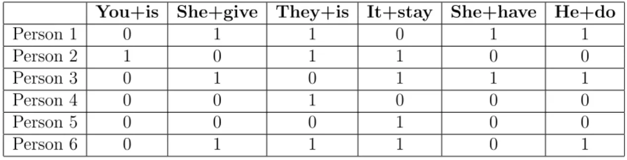
In this section, the author presents the steps for calibrating the Rasch Model. The facilitator builds a table where each column contains hits or misses for a given item. Each row shows hits or misses for a grammatical class (vide Table 2.6).
Table 2.6: Raw Scores
You+is She+give They+is It+stay She+have He+do
Person 1 0 1 1 0 1 1
Person 2 1 0 1 1 0 0
Person 3 0 1 0 1 1 1
Person 4 0 0 1 0 0 0
Person 5 0 0 0 1 0 0
Person 6 0 1 1 1 0 1
Let us understand what calibration is. If we determine that probability depends on parameters like difficulty and ability, calibration therefore is the process of determining these parameters.
In general, raw measurements do not correlate well with the model. However, Joint Likelihood Estimation can force raw data into the model, thus discovering the ability and difficulty parameters.
On the facilitator’s matrix, the cells receive value 1 if grammatical class is correct or 0 otherwise (vide Table 2.6).
(defparameter Xn
#2A((0.0 1.0 1.0 0.0 1.0 1.0) ; 1 (1.0 0.0 1.0 1.0 0.0 0.0) ; 2 (0.0 1.0 0.0 1.0 1.0 1.0) ; 3 (0.0 0.0 1.0 0.0 0.0 0.0) ; 4 (0.0 0.0 0.0 1.0 0.0 0.0) ; 5 (0.0 1.0 1.0 1.0 0.0 1.0) ; 6 ))
Using this initial data one proceeds to determine the origin of the ability and difficulty scales. To meet this goal, an iterative algorithm must force raw data onto the logistic curve. The first step of the iteration calculates row and column averages to estimate initial difficulty and ability vectors for the data matrixXn.
The hitsfunction returns a list with the average arithmetic for each line of the array Xn. The average will be the starting point for the ability calculation. The function hab_logitcalculates the initial ability vector.
(defun hits(m)
(make-array (list d0) :initial-contents (loop for i from 0 below d0
collect (loop
for j from 0 below d1
when #i(m[i,j]==1) sum 1.0 into s1 finally (return #i(s1 /d1))) )))
(defun hab_logit (vet &optional (v_logit (make-array d0))) (loop for i from 0 below d0 do
#i(v_logit[i]=log(vet[i]/(1-vet[i])))) v_logit)
The misses function returns a list with the arithemetic average of each column in the array Xn. The average will be the starting point for the difficulty calculation. The functiondif_logit produces the initial difficulty vector.
(defun misses(m)
(make-array (list d1) :initial-contents (loop for j from 0 below d1
collect (loop
for i from 0 below d0
when #i(m[i,j]==1) sum 1.0 into s1 finally (return #i(s1 / d0))) )))
(defun dif_logit (vet &optional (v_logit (make-array d1))) (loop for i from 0 below d1 do
#i(v_logit[i]=log((1-vet[i])/vet[i]))) v_logit)
element. The functionprobabilitycalculates the odds given by equation 2.2. The odds for each difficulty/ability pair is stored in a two dimensional array.
(defun avg-vector (vet) (loop for x across vet
sum x into s count x into c finally (return (/ s c)))) (defun adj_dif_logit (vet avg)
(map ’vector (lambda(x) (- x avg)) vet))
(defun probability (A Dadj &optional (m (make-array (list d0 d1)))) (loop for i from 0 below d0 do
(loop for j from 0 below d1 do
#i(m[i,j] := (exp (A[i] - Dadj[j])) / (1.0 + (exp (A[i] - Dadj[j])))) )) m)
In order to update the ability and difficulty vectors, one must calculate the residual between the current and the previous probability matrix.
(defun residual(mi me &optional
(rs (make-array (list d0 d1))))
(loop for i from 0 below d0 do
(loop for j from 0 below d1 do
#i(rs[i,j] := mi[i,j] - me[i,j]) ))
rs)
(defun residual_sum(m &optional
(sum (make-array d0)))
(loop for i from 0 below d0 do
(loop for j from 0 below d1 do
#i(sum[i] := sum[i] + m[i,j]) ))
sum)
(defun variance (m &optional
(mv (make-array (list d0 d1)))) (loop for i from 0 below d0 do
(loop for j from 0 below d1 do
#i(mv[i,j] := m[i,j] * (1 - m[i,j])) )) mv)
(defun sum_row_mat(m)
(make-array (list d0) :initial-contents (loop for i from 0 below d0 collect
(loop for j from 0 below d1 sum #i(-m[i,j])))) )
(defun sum_col_mat(m)
(make-array (list d1) :initial-contents (loop for j from 0 below d1 collect
(loop for i from 0 below d0 sum #i(-m[i,j])))) )
After summing up the residual and variance for each of the two dimensional arrays along each row, one is ready to update the difficulty and ability vectors.
(defun newA(A rs vrc &optional
(nAbil (make-array d0))) (loop for i from 0 below d0 do
#i(nAbil[i] := A[i]-rs[i]/vrc[i])) nAbil)
(defun newD (D rs vrc &optional
(nDif (make-array d1))) (loop for i from 0 below d1 do
#i(nDif[i] := D[i]-rs[i]/vrc[i]) ) nDif)
These steps must be repeated until the sum of the squares of the residuals becomes sufficiently small.
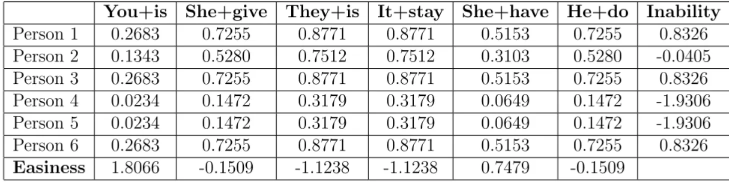
Table 2.7: Probabilities
You+is She+give They+is It+stay She+have He+do Inability
Person 1 0.2683 0.7255 0.8771 0.8771 0.5153 0.7255 0.8326 Person 2 0.1343 0.5280 0.7512 0.7512 0.3103 0.5280 -0.0405 Person 3 0.2683 0.7255 0.8771 0.8771 0.5153 0.7255 0.8326 Person 4 0.0234 0.1472 0.3179 0.3179 0.0649 0.1472 -1.9306 Person 5 0.0234 0.1472 0.3179 0.3179 0.0649 0.1472 -1.9306 Person 6 0.2683 0.7255 0.8771 0.8771 0.5153 0.7255 0.8326
Easiness 1.8066 -0.1509 -1.1238 -1.1238 0.7479 -0.1509
Using this initial data one proceeds to determine the origin of the ability and difficulty scales. To meet this goal, an iterative algorithm must force raw data onto the logistic curve.
The facilitator adds a row for the List classifier to the table. The Condorcet-List classifier selects all classifiers with probabilities above 0.5 and promotes a votation among them, choosing the plurality winner class.
Table 2.8: Probabilites of Voters
You+is She+give They+is It+stay She+have He+do
Person 1 0.7255 0.8771 0.8771 0.5153 0.7255
Person 2 0.5280 0.7512 0.7512 0.5280
Person 3 0.7255 0.8771 0.8771 0.5153 0.7255 Person 4
Person 5
Person 6 0.7255 0.8771 0.8771 0.5153 0.7255
In table 2.8 all voters with a hitting probability less than 0.5 were removed. After this filtering process the majority vote was realized. The majority vote was obtained through a consideration of the vote of each voter, presented in table 2.6. In the case of a draw or that there does not exist a single vote for the item, the value of zero is attributed for the Condorcet-List vote. Therefore, the Condorcet-List vote is presented in table 2.9.
Table 2.9: Condorcet-List Voter
You+is She+give They+is It+stay She+have He+do
Condorcet-List 0.0 1.0 1.0 1.0 1.0 1.0
voters.
Table 2.10: Hit Probabilities
You+is She+give They+is It+stay She+have He+do
Condorcet-List 0.3999 0.9117 0.9644 0.9645 0.8168 0.9117
Chapter 3
Lisp and Mathematics
In this chapter, the author will provide the content necessary for an adequate understand-ing of all followunderstand-ing chapters.
Which programming methodology should I use to prevent my programs from becoming obsolete? The author presents the reasons why Lisp was chosen as the language for the development of this work.
Computer languages have, in general, a very complex syntax. A Python programmer, for instance, must learn many syntactical variants for calling up a function: The function that calculates the logarithm has a prefix notation, while the functions that perform multiplications and additions obey infix syntax rules. Even the four basic arithmetic operations do not obey the same syntax rules, since they have different precedence and associativity.
>>> import math
>>> math.log(3,4)
0.7924812503605781
>>> (3+4)*(5+6+7)*8
1008
application cannot adapt the compiler to fit the problem they are dealing with.
Instead of accepting an arbitrary syntax, the Lisp community adopted a kind of sym-bolic expressions, which evolved from a mathematical notation proposed by Lukasiewicz in 1920. In mathematics, basic constructions and transformation rules are kept to a min-imum. Thislex parsimoniæhas many consequences. The first one is that few rules can classify all symbolic expressions:
1. Numerals have traditional notation: 3, 3.1416, -8, etc.
2. Symbols are sequences of characters that cannot be interpreted as numbers and do not contain brackets: sin, x, y, *ops*, etc.
3. Quoted lists such as ’(a b e) represent sequences of objects. 4. Unquoted lists such as (log 8 2) denote function calls.
5. Abstractions such as (lambda(x y) (log (abs x) y)) define functions. The sequence of symbols (x y) is called a binding list, and the expression (log (abs x) y) is the body of the abstraction.
Any variable that appears in the binding list is said to be bound. Free variables occur in the body of the abstraction but not in the binding list.
Another consequence of its mathematical foundations is that Lisp has a clear and simple semantics. The rules of computation are based on a Mathematical system called the Lambda Calculus.
α-conversion Changing the name of a bound variable produces equivalent expressions. Therefore, (λ(x)x) and (λ(y)y) are equivalent.
β-reduction ((λ(x)E)v) can be reduced to E[x:=v].
Lisp has a Read Eval Print Loop (REPL) that performs β-reduction over symbolic expressions in order to simplify their forms. In theβ-reduction process, the first element of a list can be considered as a function or a macro.
CL-USER(1): (log 3 4)
0.79248124
CL-USER(2): (* (+ 3 4) (+ 5 6 7) 8)
1008
One immediate advantage of its mathematical foundations is that Lisp is unlikely to become obsolete. This means that one may expect that a language like Python or Fortran to suffer changes without backward compatibility. One can even expect that Python or Fortran would be phased out. However, Lisp code written many decades ago can be easily run in a modern computer. Besides this, since Lisp does not change, computer scientists can work on Lisp compilers for many decades, which results in fast and robust code.
Let (lambda(x) (- (/ (* (+ x 40) 9) 5.0) 40)) represent the function
λ(x)(x+ 40)×9/5 + 40 that converts Celsius degrees to Fahrenheit. One can store this function in a functional symbol, as one can see below.
(setf (symbol-function ’c2f)
(lambda(x)
" Celsius to Fahrenheit"
(- (/ (* (+ x 40) 9) 5.0) 40)))
#| From REPL:
CL-USER(1): (c2f 100)
212.0
|#
3.1
Tool for natural language processing
One tool used for natural language processing is rasp3os[2]. The system is written in Lisp, with a few low level components in C. The distribution, according to the README, includesunix shell scripts for running the whole analysis system, or just the parser. Let us see how to install the system, and test it using the provided shell scripts.
One must operate the rasp3os through the command-line interface. A shell command language interpreter (CLI) is a tool for interacting with the operating system where the client issues commands in the form of successive lines of text. A search on the Internet shows that there are plenty of tutorials on the CLI[3], but a person who is not fluent in shell script will be better off asking help from a computer science major.
In order to study and use rasp3os, the interested reader must download the installer from the distribution page[2]. After expanding the archive, all one needs to do is type makeinto the shell. The next step is to test the scripts.
~/rasp3os/scripts$ echo "Helen, thy beauty is to me\
like those Nicean barks of yore" | ./rasp.sh -p’-os -u’
(|Helen_NP1| |,_,| |thy_APP$| |beauty_NN1|
|be+s_VBZ| |to_II| I+_PPIO1 |like_II|
|those_DD2| |Nicean_NP1| |bark+s_NN2|
|of_IO| |yore_NN1|) 1 ; (-25.427)
sparkle: 1
("S" ("NP" "Helen") "," ("NP" "thy" "beauty")
("VP" "be+s" ("PP" "to" "I+")
("PP" "like"
("NP" "those" "Nicean" "bark+s"
("PP" "of" ("N1" "yore"))))))
From the above output, one can readily see that rasp performs two sorts of text analysis, tagging and syntax.
the early 1980s. The latest version of the tagger, CLAWS4, was used to perform Part-of-speech tagging of circa 100 million words of the British National Corpus. This very near complete and robust tagger is part-and-parcel of the rasp3os package.
• Syntax. After tagging, the rasp system builds the text syntax tree. The system can produce many syntactic representations for a given tagged text. The representation shown above is convenient as it can be read back into a Lisp system for further processing.
The author will look closer at Tagging and Syntax in chapter 4.
3.2
Emacs
In order to simplify the communication style, let us assume that Nia, a programmer, has already checked the functionality of rasp, and decided to try her hand at natural language processing. In order to work with Lisp, Nia should install the following packages:
1. A Lisp compiler, such as sbcl[4] or clozure.
2. Emacs, a customizable, self-documenting display editor. 3. Slime[5], the superior Lisp interaction mode for Emacs. 4. Quicklisp[6], a tool for installing Lisp applications.
A linguist that is not conversant with Lisp should ask for help from a computer science major when installing and configuring the above systems.
An environment used frequently for developing Lisp programs is Emacs, a text editor that one can configure with macros written in a dialect of Lisp designed for processing text. Emacs has a Superior Lisp Interaction Mode, also known as slime. Make sure to ask the computer science major that is helping you to check whetherslime is configured correctly.
into the emacs minibuffer (a one line buffer at the bottom of the page). From the eshell, she uses the command line interpreter to check whether slime is correctly installed.
~/wrk/ $ cd ~ # Comments start with the hash symbol
~ $ ls quicklisp/ # checks for quicklisp
asdf.lisp setup.lisp cache
dists quicklisp tmp
~ $ cd .emacs.d/ # visits the emacs directory
~/.emacs.d $ ls # make sure that slime is installed
auto-save-list eshell lisp slime
~/.emacs.d $ ls lisp # OS-x needs this application
exec-path-from-shell.el
The commandC-x C-freads the~/.emacsname from the minibuffer, creating a new buffer for the ~/.emacs configuration file.
Find file: ~/.emacs
Just like any other program, Emacs can benefit from a configuration file in order to work correctly. Therefore, Nia types the following script into the .emacs configuration file:
;; .emacs for scripting in sbcl
(global-visual-line-mode t) ; wrap word at the end of line
(setq inhibit-splash-screen t)
(setq inhibit-startup-message t)
(set-face-attribute ’default nil :height 160)
;; Necessary to make emacs PATH equal to the shell PATH
(add-to-list ’load-path "~/.emacs.d/lisp")
(require ’exec-path-from-shell)
(exec-path-from-shell-initialize)
(setq linum-format "%4d ")
(global-linum-mode 1)
(setq inferior-lisp-program "/usr/local/bin/sbcl")
(add-to-list ’load-path "~/.emacs.d/slime/")
(require ’slime)
Computational systems that perform complex tasks such as natural language pro-cessing are large and have dependencies scattered all over the web. Richard Stallman suggests that learners of such a system should start their studies by testing open source applications, then proceed to modify them to fit the situation at hand.
3.3
Quicklisp
The quicklisp system provides the tools to download and install packages written in Com-mon Lisp. Therefore, the interested reader should visit the distribution page[6] and install quicklisp before any attempt at experimenting with natural language processing.
Let us examine how Nia performed the installation and configuration of quicklisp. She downloads thequicklisp.lisp installer and places it in her home directory.
~$ sbcl # Nia has already installed sbcl
This is SBCL 1.2.11, an implementation of ANSI Common Lisp.
* (load "quicklisp.lisp")
T
* (quicklisp-quickstart:install)
NIL
* (ql:add-to-init-file)
the instructions given in the readme file.
From Emacs, Nia press C-x C-f to open the ~/.sbclrc configuration file, and finds it in the following situation:
;;; The following lines added by ql:add-to-init-file:
#-quicklisp
(let ((quicklisp-init (merge-pathnames "quicklisp/setup.lisp"
(user-homedir-pathname))))
(when (probe-file quicklisp-init)
(load quicklisp-init)))
The only command present in the.sbclrcconfiguration file was introduced there by quicklisp. Then Nia adds a few Lisp instructions to this nearly empty .sbclrc file, in order to profit from a better environment for experimenting with Common Lisp.
Lisp has a read eval print loop (REPL). This means that the Lisp compiler reads an expression, evaluates it and prints the result. After installing sbcl and quicklisp, Nia can start the REPL from a unix shell and test the whole system as shown below. She also installs thetagger package to get acquainted with the normal Lisp installation process.
~/tg$ sbcl
* (require :sb-aclrepl) ;; use semicolon for comments
("SB-ACLREPL")
CL-USER(2): (ql:quickload :tagger)
(:TAGGER)
CL-USER(3): (tag-analysis:tag-string
"The white cat also catches mice.")
The white cat also catches mice.
CL-USER(3): (ql:quickload :infix)
To load "infix":
Load 1 ASDF system:
infix
; Loading "infix"
;;; ********************************************
;;; Infix notation for Common Lisp.
;;; Written by Mark Kantrowitz.
;;; ********************************************
(:INFIX)
CL-USER(4): #i(1.8 * 38+32)
100.4
CL-USER(5): (exit) ;; quit Lisp
Nia starts sbcl from the unix shell. The default prompt is an asterix, which is far from ideal, since it does not provide any information concerning the environment. The command
(require :sb-aclrepl)
introduces a better prompt. Note that Lisp expressions always have the form: open parenthesis, operation, arguments, close parenthesis. In the present case, the operation is require, and the sole argument is the :sb-aclreplkeyword. If Nia adds this improved prompt into the .sbclrcconfiguration file, Lisp activates it at each startup.
;;; The following lines added by ql:add-to-init-file:
#-quicklisp
(let ((quicklisp-init (merge-pathnames "quicklisp/setup.lisp"
(user-homedir-pathname))))
(when (probe-file quicklisp-init)
;; Infix notation for Lisp
(ql:quickload :infix)
;; A better Read Eval Print Loop
(require ’sb-aclrepl)
;; Let us turn the debugger off
(defun debug-ignore (c h)
(declare (ignore h))
(format t "~a" c)
(abort))
(setf *debugger-hook* #’debug-ignore)
Infix notation. Lisp arithmetic operations have prefix notation, like any other expres-sion in the language. Instead of writing 9*(38+40)/5.0-40 for converting 38 Celsius degrees to Fahrenheit, a Lisp programmer would type(- (/ (* 9 (38+40)) 5.0) 40) to reach the same result. By adding
;; Infix notation for Lisp
(ql:quickload :infix)
to the.sbclrcconfiguration file, Nia installs infix notation in Lisp. Then, she can write the temperature conversion formula thus:
#i(9*(x+40)/5.0-40)
3.4
Emacs commands
One can use emacs through menus. However, advanced users prefer shortcut key strokes. In the following cheat sheet, κcan be any key, Spc denotes the space bar,C- is the Ctrl prefix, and M- represents the Alt prefix.
• C-κ – Press and release Ctrland κsimultaneously C-s – search a text
C-k – kill a line
C-Spc then move the cursor – select a region M-w save selected region into a ring
C-w kills region
C-y insert killed or saved region C-g cancel minibuffer reading
• C-x C-κ – KeepCtrl down and press x and κ
C-x C-f – open a file into a new buffer C-x C-s – save file
C-x C-c – exit emacs
• C-x κ – Press and release Ctrl and x together, then press κ
C-x b – switch buffers
C-x 2 – split window into cursor window and other window C-x o – jump to the other window
C-x 1 – close the other window C-x 0 – close the cursor window
When text is needed for carrying out a command, it is read from the minibuffer. For instance, if Nia pressesC-sfor searching a text, the text is read from the minibuffer. For giving up on a command, she may pressC-g.
moves the cursor to the insertion place, and presses the C-y shortcut. To copy a region, Nia pressesC-Spcand moves the cursor to select the region. Then she presses M-wto save the selection into the kill ring. Finally, she takes the cursor to the destination where the copy is to be inserted and issues theC-y command.
3.5
Arithmetic operations
In order to get acquainted with Emacs, Nia entered the editor and pressed C-x C-f to create the fahrenheit.lisp buffer. She typed the program below into the buffer. ;; File: fahrenheit.lisp
(defun c2f(c)
"Celsius to Fahrenheit" ;optional documentation
(- (/ (* (+ x 40) 9) 5.0) 40))
(defun f2c(x)
#i(5.0*(x+40)/9-40))
Function c2f converts Celsius readings to Fahrenheit. The defun macro, that defines a function, has four components, the function id, a parameter list, an optional documen-tation, and a body that contains expressions and commands to carry out the desired calculation. Comments are prefixed with a semicolon. In the case of c2f, the id is c2f, the parameter list is (x), and the body is (- (/ (* (+ x 40) 9) 5.0) 40).
Lisp programmers prefer the prefix notation: open parentheses, operation, arguments, close parentheses. Therefore, in c2f, (+ x 40) adds x to 40, and (* (+ x 40) 9) mul-tipliesx+ 40 by 9.
It is possible to use macros for automatic conversion from any syntax to the prefix form. For instance, the definition of f2c, that converts Fahrenheit readings to Celsius, the body is in the infix notation[7] of highschool precalculus.
the Lisp REPL, Nia can load the program and call any application that comes with Lisp, or she defined herself.
CL-USER(1): (load "fahrenheit.lisp")
T
CL-USER(2): (c2f -40)
-40.0
CL-USER(3): (documentation ’c2f ’function)
"Celsius readings to Fahrenheit"
CL-USER(4): (f2c 100)
37.77778
Nia is working with two buffers, one running Lisp and the other containing a file. There are two ways for switching from one buffer to the other. Nia can go to the Buffers > myfile menu and choose the destination from a list of options. A better method is the C-x b command (press and release Ctrl x, then type b. The minibuffer shows the first option. Nia can scroll through the options by pressing the up arrow key. Once she finds the destination buffer by this process, she presses Enter to go to that point.
There is also a third option for switching between buffers. Initially, Nia splits the window withC-x 2and, afterwards, uses the C-x bto visit the fahrenheit.lispbuffer on one of the two windows.
;; CtoF.lisp
(defun c2f(x)
#i(9*(x+40)/5.0-40))
CL-USER(1): (load "CtoF.lisp")
T
CL-USER(2): (c2f 37.77778)
Now she has the two buffers in front of her, each with its own window. Nia can use the mouse for jumping from one window to the other.
(defun wday( y m mday &optional
(yfix (floor (- 14 m) 12))
(mm #i(m+ 12*yfix -2))
( yy (- y yfix))
(century (- (floor yy 100))))
(mod (+ yy (floor #i(13*mm - 1) 5)
(floor yy 4) century
(floor yy 400) mday) 7))
The above program calculates the day of the week through Zeller’s congruence. The &optional keyword introduces pairs of variable/values. For instance, the pair (yy (- year yfix)) establishes that the variable yy may be initialized with the re-sult of the (- y yfix) calculation. The floor function performs the integer divisions required by the algorithm.
3.6
The let-form
The let-form introduces local variables through a list of(id value) pairs. (defun zr(y m d &optional
(ax (floor (- 14 m) 12))
(mm (+ m (* 12 ax) -2))
(yy (- y ax)) )
(let ( ;open list of local variables
(c (- (floor yy 100))) ;first pair of (id value)
(ly (floor yy 4)) ;second pair of (id value)
) ;close list of local variables
(mod (+ yy (floor (- (* 13 mm) 1) 5)
ly c
In the basic let-form, a variable cannot depend on previous variables that appear in the local list. In the let-star form, one can use previous variables to calculate the value of a variable, as noted in the definition below.
(defun zlr(y m d)
(let* ( (ax (floor (- 14 m) 12)) ;id= ax
(mm (+ m (* 12 ax) -2)) ;id= mm
(yy (- y ax)) ;id= yy
(c (- (floor yy 100))) ;id= c
(ly (floor yy 4)) ;id= ly
) ;close list of local variables
(mod (+ yy
(floor (- (* 13 mm) 1) 5)
ly (floor yy 400) d) 7)))
When using a let-form, the programmer must bear in mind that it needs parentheses for grouping together the set of (id value) pairs, and also parentheses for each pair. Therefore, one must open two parentheses in front of the first pair, one for the list of pairs and the other for the first pair.
A common error when dealing with the let-form is to forget the parentheses that group local variables together. Besides this, learners often leave out the parentheses that associate each variable with its value. Therefore, one is advised to study the syntax of the let-form carefully, to avoid these two types of error.
3.7
Lists
In Lisp, there is a data structure called list, that uses parentheses to represent nested sequences of objects.
;;File: probability.lisp
(setf (get ’noun ’rs)
(setf (get ’det ’rs)
’( ((def 0.5 the)/)
((indef 0.5 a)/)
((indef 0.5 an)/)) )
(setf (get ’np ’rs)
’( ((np 0.5) = (n))
((np 0.5) = (det) (n))))
In the above file, thesetfmacro associates lists to the’rsindicator of the symbolsnoun, det and np. When these lists represent data, and not programs, they must be prefixed with a quotation mark.
From its very outset, Lisp connects indicators to every symbol. The symbols to-gether with their indicators can be seen as a tabular data base called a property list. A property list has a number of entries, each one associated to an indicator. For instance, (get ’np ’rs)associates a list of clauses with an “rs” indicator appended to the symbol np. The command
(setf (get ’np ’rs)
’( ((np 0.5) = (n))
((np 0.5) = (det) (n))))
saves the quoted list into thers storage location associated with symbolnp in such a way that it can be retrieved with the (get ’np ’rs)function.
The functions (car s) and (cdr s) are called selectors, and are used to access the parts of a list: (car s) produces the first element of the s storage, while (cdr s) is the result of removing the first element from s. Combinations of (car s) and (cdr s) can fetch any element from a list. For instance, (car (cdr ns)) produces the second element.
CL-USER(1): (load "probability")
T
CL-USER(2): (get ’np ’rules)
CL-USER(3): (car (get ’np ’rules))
((NP 0.5) = (N))
CL-USER(4): (car (cdr (get ’np ’rules)))
((NP 0.5) = (DET) (N))
Besides the two selectors, lists have a constructor: (cons x xs) builds a list whose first element isx, and the remaining elements are grouped inxs.
CL-USER(5): (cons ’((n 0.5 mouse device)/) (get ’n ’rules))
(((N 0.5 MOUSE DEVICE) /) ((N 0.5 CAT) /) ((N 0.5 MOUSE) /))
CL-USER(6): (get ’n ’rules)
(((N 0.5 CAT) /) ((N 0.5 MOUSE) /))
One has learned previously that lists must be prefixed by the special operator quote, in order to differentiate them from programs. To make a long story short, a quote prevents the evaluation of a list or symbol.
A backquote, not to be confused with quote, also prevents evaluation, but the back-quote transforms the list into a template. When there appears a comma in the template, Lisp evaluates the expression following the comma and replaces it with the result. If a comma is immediately followed by@, (at-sign), then the expression following the at-sign is evaluated to produce a list. This list is spliced into place in the template. The examples below will make things clearer.
CL-USER(8): ‘(np ,(car (get ’det ’rules)) plus noun)
(NP (DET 1.0 THE) PLUS NOUN)
CL-USER(9): ‘(np ,@(car (get ’det ’rules)) plus noun)
(NP DET 1.0 THE PLUS NOUN)
(defmacro def(category &rest rs)
‘(setf (get ’,category ’rules) ’,rs))
(def n ((n 0.5 cat)/) ((n 0.5 mice)/) )
(def det ((det 1.0 the)/) )
(def vbz ((vbz 1.0 chases)/) )
(def vp ((vp 1.0) = (vbz) (np)) )
(def np ((np 0.5) = (n)) ((np 0.5) = (det) (n)) )
(def sentence ((sentence 1.0) = (np) (vp)) )
In the above macro definition, the keyword&restgroups all remaining parameters into a list that the body of the macro can refer to through the variable that follows the keyword, in this case the variable isrs.
3.8
Packages
Nia wants to transform a string of characters into a list of words. This can be done through theppcre library.
(ql:quickload :cl-ppcre)
(defpackage :xr (:use :cl :cl-ppcre))
(in-package :xr)
(defparameter ws "[A-Za-z][a-z]*")
(defparameter nums "-?[0-9]+\.?[0-9]*")
(defun tokenize(x) (all-matches-as-strings ws x))
CL-USER(1): (load "pkg.lisp")
T
CL-USER(2): (in-package :xr)
#<PACKAGE "XR">
XR(3): (tokenize "the black cat chases mice.")
("the" "black" "cat" "chases" "mice")
Name clash is the first problem that one needs to solve when dealing with large projects. The system may have many collaborators, often working in places distant from one an-other. Even a lone ranger in programming needs to use libraries created by other people, as for example those libraries made available on quicklisp. Packages avoid that a person use an id that is already taken.
In the above example, Nia defined the package xr, that uses definitions from the cl and cl-ppcre packages. She declared that both her program and the REPL are inside the xr package. Since the REPL is inside the xr package, which does not know how to exit, Nia prefixed the cl-user::exit procedure with thecl-user package id.
Initially, thexrpackage starts out with only three names: thewsandnumsparameters and thetokenize function.
The all-matches-as-strings function tokenizes a string, producing a list of words. A regular expression, regexp for short, determines what a word is. The regexp "[A-Za-z][a-z]*" states that a word starts with a letter from A to Z or from a to z ("[A-Za-z]") followed by zero or more[a-z] letters. The asterisk mark that appears in the definition ofnumbersmakes the previous character optional. The plus sign in[0-9]+ means that numbers have at least one digit.
3.9
The cond-form
Now that Nia knows how to tokenize a text with cl-ppcre, she needs a function that calculates the average size of the words of the text.
(defun avg(ws &optional (acc 0.0) (sz 0))
(cond
( (and (null ws) (> sz 0)) ;;1st clause condition
(/ acc sz) ;;action
);;end of 1st clause
( (null ws) ;;2nd clause condition
0.0) ;;action
( (consp ws) ;; 3rd clause condition
(+ (length (car ws)) acc) ;;
(+ sz 1)) )
);;end cond
);;end defun
The cond-form is used to control conditional execution, based on a set of clauses. Each clause has a condition followed by a sequence of actions. Lisp starts with the top clause, and proceeds in decending order. It executes the first clause whose condi-tion produces a value different from NIL. For instance, the first clause condicondi-tion is the (and (null ws) (> sz 0)) predicate. Since the predicate (null ws) returns T (true) for an empty ws, this condition tests whether the ws list is emptyand sz is greater than zero. Immediately after a true condition, the cond form executes the corresponding action, which is(/ acc sz) when dealing with the first clause.
The symbol nil represents both the empty list and the false boolean value. To make a long story short, the Lisp word for false is nil, which also represents the empty list. To better understand the above snippet, let us follow the execution of the (avg ’("a" "bb" "ccc")) call.
user call: (avg ws= ("a" "bb" "ccc") acc= 0.0 sz= 0.0)
1st and 2nd clauses fail, becase ws is not nil
3rd clause call: (avg ws= ("bb" "ccc") acc= 1.0 sz= 1.0)
1st and 2nd clauses fail because ws is not nil
3rd clause call: (avg ws= ("ccc") acc= 3.0 sz= 2.0)
1st and 2nd clauses fail together
3rd clause call: (avg ws= nil acc= 6.0 sz=3.0
1st clause succeeds because ws= nil and sz>3
1st clause executes (/ acc sz) producing the result.
3.10
format
Since space is limited, let us restrict the study of output to three situations, writing on the screen, superseding an existing file, and appending text to an existing file.
• Writing on the screen.
(defun greeting(name)
(format t "Hello, ~a~%" name))
• Create a new file, supersede if it exists.
(defun greeting(name file)
(with-open-file
(out file :direction :output
:if-exists :supersede)
(format out "Hello, ~a~%" name)))
• Append to an existing file.
(defun greeting(name file)
(with-open-file
(out file :direction :output
:if-exists :append)
(format out "Hello, ~a~%" name)))
3.11
Loops
A common method of simplifying a complex problem is to divide it into parts that share the same structure or the same type. Then a program calls up each part to be resolved, and the results from each part are combined to form the solution to the original problem. This method of problem solving is called recursion. Let us consider the mathematical definition of factorial.
n! is defined as
n = 0→ 1
It is straightforward to translate this mathematical definition to Lisp. (defun !(n)
(cond ( (= n 0) 1)
( (> n 0) (* (! (- n 1)) n))
)
)
The above function divides the problem of finding the factorial of n into two parts: calcu-lating the factorial of (n-1) and multiplying the result by n. The successive decrementation of the input n will lead the calculation to the base case, where n=0 and the solution is 1. After the recursive call, the computer must return to the second clause of the cond form, in order to perform the multiplication. This is inefficient, and should be avoided when-ever possible. Here is a new definition, that performs the multiplication before calling the factorial function on the simplified problem:
(defun factorial(n &optional (acc 1))
(cond ( (= n 0) acc)
( (> n 0) (factorial (- n 1) (* n acc)))
)
)
When the recursive call does not leave any task behind, the Lisp compiler can perform what is called tail call optimization and thus avoid the saving of information for completing the calculation.
Chapter 4
An space efficient implementation of
WAM
One of the principal problems through which this thesis is motivated is the technique of textmining. Textmining can be seen as the analysis of text, whereby information is obtained in high quality from texts by use of this technique. As will be presented in chapter 5.1 the Web finds itself overloaded with information, some of which is relevant and essential for research, whereas other information can be considered inadequate or useless for any kind of research. The extraction of necessary information is by any standard an arduous task. Thereby, the established techiques should be used as an aid to web users in order that they perform more efficient searches.
One particular technique that can be used is textmining. In order to perform this task two steps are necessary:
Tagger: The system that identifies grammatical and semantic categories of evaluated sentences, through the addition of a tag. Normally, the understanding of text should be founded upon data extract from large corpora, such as the Brown Corpora.
Syntactic Analysis/Parsing: This is the process use for analysing an input sequence in order to determine its grammatical structure in accordance with a particular formal grammar.
can be found in section 3.3.
In the following one finds an example of the program that uses a library tagger. ;; File: tag.lisp
(ql:quickload :tagger)
(use-package :tdb)
(use-package :tag-analysis)
(defun tkn(token-stream)
(multiple-value-bind
(token tag)
(next-token token-stream)
(if token
(cons (string-downcase (format nil "~a" tag)) token)
nil)))
(defun my-tagger (str)
(with-input-from-string (char-stream str)
(loop with token-stream =
(make-ts char-stream (make-instance ’tag-analysis))
for xt = (tkn token-stream)
then (tkn token-stream)
until (not xt)
collect xt)))
(defun vocabulary(str)
(let* ((s1 (my-tagger str))
(s2 (remove-duplicates s1 :test #’equal))
(s (sort s2 (lambda(x y)(string>= (car x)(car y))))))
(loop for (x . y) in s
Let us run the above program in Lisp.
CL-USER(1): (load "tag.lisp")
To load "tagger":
Load 1 ASDF system:
tagger
; Loading "tagger"
.
T
CL-USER(2): (vocabulary "I saw the man on the hill with the telescope.")
;;; Reading /home/junia/quicklisp/dists/quicklisp/software/
tagger-20140713-git/data/brown/suffix.trie ... Done.
;;; Reading lexicon from /home/junia/quicklisp/dists/quicklisp/software/
tagger-20140713-git/data/brown/lexicon.txt ...
;;; Done reading lexicon.
;;; Reading HMM from /home/junia/quicklisp/dists/quicklisp/software/
tagger-20140713-git/data/brown/brown.hmm
vbd([saw|S], S).
ppss([I|S], S).
nn([telescope|S], S).
nn([hill|S], S).
nn([man|S], S).
in([with|S], S).
in([on|S], S).
at([the|S], S).
NIL
CL-USER(3):
One observes that given the sentence “I saw the man on the hill with the telescope.” the tags were attributed based on the Brown Corpora.
implemented in a functional language based on Prolog. In the following sections some of the implemented inference engine parts will be described. The complete code is presented in Appendix I.
Let us consider the program synbench, that uses the implemented inference engine, for performing the syntactic analysis.
;; File: synbench
$ n(animal(cat,s), [cat|S], S).
$ n(animal(mouse,p), [mice|S], S).
$ det(def(the), [the|S], S).
$ vbz(vt(chase), [chases|S], S).
$ vp(vb(V, N), S0, S2) :- vbz(V, S0, S1), np(N, S1, S2).
$ np(np(none,N), S0, S1) :- n(N, S0, S1).
$ np(np(D,N), S0, S2) :- det(D, S0, S1), n(N, S1, S2).
$ sentence(s(N, V), S0, S2) :- np(N, S0, S1), vp(V, S1, S2).
$ len([], L, L) :- !.
$ len([_|Resto], L, Resp) :- plus(L1, L, 0.1), len(Resto, L1, Resp).
$ wrt(I, FF) :- mod(0, I, 100000), !, write(FF), nl.
$ wrt(I, FF).
$ parse(Text, 0, S, S) :- !, sentence(Sentence, Text, _),
write(Sentence), nl.
$ parse(Text, I, S, Res) :- one,
sentence(FF, Text, RR), nt,
I1 is I-1,
wrt(I, FF),
len(RR, 0, L),
S1 is S+L,
$ teste(N) :- cputime(X1),
parse([the, cat, chases, mice, sentence], N, 0, F),
cputime(X2),
minus(Time, X2, X1),
write(’Time ’),
write(Time), nl.
In synbench the dictionary tags were added by the librarytagger. For example, the wordcat is a noun and can be classified as animal(cat,s).
$ n(animal(cat,s), [cat|S], S).
$ n(animal(mouse,p), [mice|S], S).
$ det(def(the), [the|S], S).
$ vbz(vt(chase), [chases|S], S).
In the following, some grammar rules are proposed.
Verb Phrases: verb + noun phrases
Noun Phrases: noun
Noun Phrases: determiner + noun
Sentence: noun phrases + verb phrases
$ vp(vb(V, N), S0, S2) :- vbz(V, S0, S1), np(N, S1, S2).
$ np(np(none,N), S0, S1) :- n(N, S0, S1).
$ np(np(D,N), S0, S2) :- det(D, S0, S1), n(N, S1, S2).
$ sentence(s(N, V), S0, S2) :- np(N, S0, S1), vp(V, S1, S2).
In synbench given a quantity N of iterations teste(N) one adds the parser in loop. The act of performing tests in a loop is important, due to the fact that when one evaluates texts extracted from the Web a larger volumn of sentence have to be analysed. Therefore, the program needs to support a larger quantity of input.
CL-USER(1): (load "wam17.lisp")
T
CL-USER(2): (mini:wam)
mini-Wam
For the loading of synbench let us use sult. | ?- sult(synbench).
T
Yes
no More
Now, let us execute teste(N): | ?- teste(1000).
s(np(def(the),animal(cat,s)),vb(vt(chase),np(none,animal(mouse,p))))
Time 0.015999973
Yes
More : d
no More
The output forteste(N) is a syntactic tree of the evaluated sentence. s
________________
| |
np vp
_______ _________
| | | |
det n verb np
| | | |
the cat chases mice
S S1 S2 S3
| ?- halt.
Yes
no More
Bye!
#<PACKAGE "COMMON-LISP-USER">
CL-USER(3): (exit)
4.1
Concepts
Two concepts were essential in the development of this thesis, those being: function and relation.
Function: map an element from the domain in one and only one element of the counter domain.
Relation: is a map that can relate an element from the domain with one or more elements from the counter domain.
4.2
Enunciate the thesis
This thesis proposed the unification of the function and relation concepts as programming foundations.
Currently, there exist a implemenations which produce this union, as for example: Gambol [10], Paiprolog [11], Racklog [12], Schemelog [13], Kanren [14] among others. However, these implementations are not complete or do not function for large programs, or be it they do not optimize the use of time and space.
There exists those implementations that were written in non-mathematical languages. When the subject becomes a thesis these implementations presented two problems.
1. The implementations became obsolete very quickly, due to the fact that the language becomes obsolete.