www.nonlin-processes-geophys.net/16/533/2009/ © Author(s) 2009. This work is distributed under
the Creative Commons Attribution 3.0 License.
in Geophysics
Long’s equation in terrain following coordinates
M. Humi
Department of Mathematical Sciences, Worcester Polytechnic Institute, 100 Institute Road, Worcester, MA 01609, USA Received: 10 February 2009 – Revised: 27 July 2009 – Accepted: 27 July 2009 – Published: 7 August 2009
Abstract. Long’s equation describes two dimensional strat-ified atmospheric flow over terrain which is represented by the geometry of the domain. The solutions of this equation over simple topography were investigated analytically and numerically by many authors. In this paper we derive a new terrain following formulation of this equation which incorpo-rates the terrain as part of the differential equation rather than the geometry of the domain. This new formulation enables us to compute analytically steady state gravity wave patterns over complex topography in some limiting cases of the pa-rameters that appear in this equation.
1 Introduction
Long’s equation (Long, 1952, 1953, 1955, 1959) models the flow of stratified incompressible fluid in two dimensions over terrain. When the base state of the flow (that is the unper-turbed flow field far upstream) is without shear the numeri-cal solutions (in the form of steady lee waves) of this equa-tion over simple topography (i.e. one hill) were studied by many authors (Drazin, 1961, 1967; Durran, 1992; Lily, 1979; Peltier, 1983; Smith, 1980, 1989; Yih, 1967; Davis, 1999). The most common approximation in these studies was to set Brunt-V¨ais¨al¨a frequency to a constant or a step function over the computational domain. Moreover the values of two phys-ical parameters which appear in this equation were set to zero. (These parameters control the stratification and disper-sive effects of the atmosphere – see Sect. 2.) In this (singu-lar) limit the nonlinear terms and one of the leading second order derivatives in the equation drop out and the equation reduces to that of a linear harmonic oscillator over two di-mensional domain. Careful studies (Lily, 1979) showed that these approximations set strong limitations on the validity of the derived solutions (Peltier, 1983).
Correspondence to:M. Humi ([email protected])
Long’s equation also provides the theoretical framework for the analysis of experimental data (Shutts, 1988, 1994; Jumper, 2005) under the assumption of shearless base flow. (An assumption which, in general, is not supported by the data; Humi, 2004b.) An extensive list of references appears in (Baines, 1995; Carmen, 2002; Yih, 1980).
An analytic approach to the study of the solutions of this nonlinear equation was initiated recently by the current au-thor (Humi, 2004a, 2006, 2007). We showed that for a base flow without shear and under rather mild restrictions the non-linear terms in the equation can be simplified. We also iden-tified the “slow variable” that controls the nonlinear oscilla-tions in this equation. Using phase averaging approximation we derived for self similar solutions of this equation a for-mula for the attenuation of the stream function perturbation with height. This result is generically related to the presence of the nonlinear terms in Long’s equation. The impact that shear has on the generation and amplitude of gravity waves was investigated by us in (Humi, 2006). A new representa-tion of this equarepresenta-tion in terms of the atmospheric density was derived in (Humi, 2007).
One of the weak aspects of Long’s equation is related to the fact that the terrain is represented by the shape of the do-main and the boundary conditions. As a result the impact of different terrains on the solution of this equation can only be studied numerically. Furthermore discretization errors which occur in the representation of the terrain render it impractical to consider complex terrain. In part these errors are due to the scale of the terrain relative to the computational domain. Ac-cordingly only simple topographies which were represented by one hill were considered in the literature. Furthermore even for these simple topographies only approximate bound-ary conditions were applied at the terrain. (See discussion in Sect. 2.)
to derive new analytic insights about the solution of this equation in some limiting cases. It will make it easier also to study how the solution varies as a function of the terrain and other parameters that appear in the equation.
The plan of the paper is as follows: Sect. 2 presents a short review of Long’s equation and some aspects of its solutions. In Sect. 3 we derive the new formulation of this equation. Section 4 considers Long’s equation in some limiting cases of the parameters that govern the solution of this equation. In particular we provide a closed form analytic solution of this equation in the limiting caseµ=β=0 over general topogra-phy. A first order perturbation expansion is developed for the case of “low lying topography” with closed form expression for the stream function in integral form. We end up in Sect. 5 with a summary and conclusions.
2 Long’s equation – a short overview
In two dimensions(x, z)the flow of a steady inviscid and incompressible stratified fluid is modeled by the following equations:
ux+wz=0 (1)
uρx+wρz=0 (2)
ρ(uux+wuz)= −px (3)
ρ(uwx+wwz)= −pz−ρg (4)
where subscripts indicate differentiation with respect to the indicated variable,u=(u, w)is the fluid velocity,ρis its den-sitypis the pressure andgis the acceleration of gravity.
We can non-dimensionalize these equations by introduc-ing
¯
x = x L, z¯=
N0 U0z, u¯ =
u U0, w¯ =
LN0
U02 w
¯
ρ= ρ
¯
ρ0
, p¯= N0 gU0ρ¯0
p (5)
where L represents a characteristic horizontal length, and
U0,ρ¯0represent respectively the free stream velocity and
av-eraged base density (i.e. here ρ0¯ is a constant). N02 is an averaged value of the Brunt-V¨ais¨al¨a frequency
N2= −g ρ0
dρ0
dz (6)
whereρ0=ρ0(z)is the base density.
In these new variables Eqs. (1)–(4) take the following form (for brevity we drop the bars)
ux+wz=0 (7)
uρx+wρz=0 (8)
βρ(uux+wuz)= −px (9)
βρ(uwx+wwz)= −µ−2(pz+ρ) (10)
where
β= N0U0
g (11)
µ= U0
N0L . (12)
β is the Boussinesq parameter (Davis, 1999) (this name has nothing to do with the “Boussinesq approximation”) which controls stratification effects (assumingU06=0) andµis the long wave parameter which controls dispersive effects (or the deviation from the hydrostatic approximation). In the limit
µ=0 the hydrostatic approximation is fully satisfied (Smith, 1980, 1989).
In view of Eq. (7) we can introduce a stream function9
so that
u=9z, w= −9x. (13)
Using this stream function we can rewrite Eq. (8) as
J{ρ, 9} =0 (14)
where for any two (smooth) functionsf, g J{f, g} = ∂f
∂x ∂g ∂z −
∂f ∂z
∂g
∂x (15)
Equation (14) implies that the functionsρ, 9 are dependent on each other and we can express each of them in terms of the other. Thus we can write9 as9(ρ)(orρasρ(9); Humi, 2007).
After a long algebra one can derive the following equation for9(Dubreil, 1934; Long, 1953; Davis, 1999)
9zz+µ29xx−N2(9)
z+β
2
9z2+µ29x2
=S(9) (16)
where
N2(9)= −ρ9
βρ (17)
is the nondimensional Brunt-V¨ais¨al¨a frequency. We observe that in this definitionN2is a function of9. (As a result it can be an additional source of nonlinearity in Eq. 16.) This is in contrast to the previous definition of this quantity in Eq. (6) which depends only on the base state. In the following we assume without loss of generality that the direction of base flow is from left to right along the x-axis. Furthermore we assume it to be a function ofzonly.
S(9)is some unknown function which is determined from the base flow. To carry out this determination ofS we con-sider Eq. (16) asx→−∞and express the left hand side of this equation in terms of 9 only. (Assuming that distur-bances do not propagate far upstream; Baines, 1995; Yih, 1980). Equation (16) is referred to as Long’s equation.
For example if we let lim
i.e. consider a shearless base flow with lim
x→−∞u(x, z)=1 then S (9)= −N2(9)
9+β
2
(19) and Eq. (16) becomes:
9zz+µ29xx−N2(9)
z−9+β
2
92z+µ29x2−1
=0. (20) It is evident from this derivation that different profiles for the base flow asx→−∞ will lead to different forms of S(9)
(Humi, 2006).
For a general base flow in an unbounded domain over to-pography with shapef (x)and maximum heightH0the
fol-lowing boundary conditions are imposed on9
lim
x→−∞9(x, z)=90(z) (21)
9(x, τf (x))=constant, τ = H0N0
U0 (22)
where the constant in Eq. (22) is (usually) set to zero. As to the boundary condition atx→∞it is appropriate to set
lim
x→∞9(x, z)=90(z)
(in spite of the fact that Long’s equation contains no dissipa-tion terms). However over finite computadissipa-tional domain only radiation boundary conditions can be imposed in this limit. Similarly asz→∞it is customary to impose (following Dur-ran, 1992) radiation boundary conditions. (The imposition of these boundary conditions is discussed in detail in Sect. 4.1.)
For the perturbation from the shearless base flow
η=9−z (23)
Equation (20) becomes
ηzz−α2η2z+µ2
ηxx−α2ηx2
−N2(η) (βηz−η)=0 (24) where
α2= N 2(9) β
2 . (25)
We observe that when |τ|≪1 the boundary condition Eq. (22) can be approximated by
η (x,0)= −τf (x). (26)
WhenN is constant eq. (24) is invariant with respect to translations inx, zand hence admits self-similar solutions of the formη=f (kx+mz)(Humi, 2004a). These solutions are interpreted as gravity waves that are generated by the flow over the topography.
From a numerical point of view it is a common practice (Durran, 1992; Lily, 1979; Davis, 1999) to solve Eq. (24) in the limitβ=0 andµ=0 with constantN over the domain. However observe that the definition ofNin Long’s equation
is given by Eq. (17) and it depends on9. In some other nu-merical simulations the computational domain is divided into subdomains whereN is constant in each subdomain but this led to numerical instabilities at the interface between these subdomains.
In these limits Eq. (24) reduces then to a linear equation
ηzz+N2η=0. (27)
We observe that the limitβ=0 can be obtained either by let-tingU0→0 orN0→0. In the following we assume that this
limit is obtained asU0→0 (so that stratification persists in
this limit and the leading term inN0is not zero).
Equation (27) is a singular limit of Long’s equation as one of the leading second order derivatives drops whenµ=0 and the nonlinear terms drops out whenβ=0 andN is con-stant. This approximation and its limitations were considered numerically and analytically (Drazin, 1967; Durran, 1992; Humi, 2004a, 2006) and was found to be justified only under strong restrictions even under the assumption that the base flow is shearless. Nevertheless it is used routinely in the actual analysis of atmospheric data (Shutts, 1988; Jumper, 2005; Baines, 1995).
The general solution of Eq. (27) is
η(x, z)=q(x)cos(N z)+p(x)sin(N z) (28) where the functionsp(x), q(x)have to be determined so that the the boundary conditions derived from Eqs. (22), (26) and the radiation boundary conditions are satisfied. These lead in general to an integral equation forp(x)andq(x)and it easy to show (Davis, 1999) thatp(x)=H[q(x)]whereH[q(x)]
is the Hilbert transform ofq(x). The boundary condition on the terrain becomes;
q(x)cos(τ Nf (x))+H[q(x)]sin(τ Nf (x))=−τf (x) . (29) This integral equation has to be solved numerically (Drazin, 1961; Durran, 1992; Davis, 1999; Kar, 1995).
3 Terrain following formulation
To derive a terrain following formulation of Long’s equation which incorporates the terrain in the coefficients of the dif-ferential equation (rather than the shape of the domain) we introduce Gal-Chen transformation. If the height of the (bot-tom) terrain is described by a sufficiently smooth function
z=h(x)and the height of the computational flow region is finite, i.e.h(x)≤z≤H, whereHis a constant, then this trans-formation is given by
¯
x=x, z¯=H z−h(x)
H−h(x). (30)
Under this transformation we have
∂ ∂x =
∂ ∂x¯ +G
12 ∂ ∂z¯,
∂ ∂z =
1
√
G ∂
where 1
√
G =
H
H−h(x), G 12
= √1
G
¯
z H −1
h′(x). (32) Furthermore the expression of the Laplace operator becomes
¯
∇2= ∂
2 ∂x¯2+
1
G+
G12 2 ∂2
∂z¯2+2G 12 ∂2
∂x∂¯ z¯+
"
∂G12 ∂x¯ +G
12∂G12 ∂z¯
#
∂
∂z¯. (33)
Under this transformation the continuity Eq. (7) becomes
∂u ∂x¯ +G
12∂u ∂z¯ +
1
√
G ∂w
∂z¯ =0. (34)
However, if we introduce
v=√1 G
w+√GG12u (35)
then it is a simple algebra to show that Eq. (34) can be rewrit-ten as
∂ ∂x¯
√
Gu+ ∂ ∂z¯
√
Gv=0. (36)
From this equation we see that we can introduce a “terrain following stream function”ψso that
¯
u=√Gu= ∂ψ ∂z¯, v¯=
√
Gv= −∂ψ
∂x¯. (37)
Multiplying Eq. (8) by√Gwe can rewrite this equation in the following form:
¯
u∂ρ ∂x¯ + ¯v
∂ρ
∂z¯ =0. (38)
Using Eq. (37) this can be rewritten as
¯
J{ρ, ψ} =0 (39)
where J¯ is defined as in Eq. (15) but with differentia-tions with respect to (x,¯ z)¯ . Equation (39) implies that
ρ(x,¯ z)¯ =ρ(ψ (x,¯ z))¯ (and vice versa).
To eliminate the pressure term from Eqs. (9) and (10) we differentiate Eq. (9) by z and apply the operator µ2∂x∂ to Eq. (10) and subtract. We obtain
βµ2ρx(uwx+wwz)−βρz(uux+wuz)+
βµ2ρ(uwx+wwz)x−βρ(uux+wuz)z=−ρx. (40) Using Eq. (8) the first two terms in this equation can be writ-ten as
βµ2ρx(uwx+wwz)−βρz(uux+wuz)=β h
µ2(−ρzwwx+
ρxwwz)−ρzuux+ρxuuz=
β
2 h
ρx(u2+µ2w2)z−
ρz
u2+µ2w2
x i
= β
2√G
ρx¯
u2+µ2w2 ¯ z−
ρ¯z
u2+µ2w2 ¯ x i
= β
2√GJ¯{ρ, u 2
+µ2w2}. (41)
Using Eqs (35) and (37) to re-expressu2+µ2w2we have
β
2√GJ¯
n
ρ, u2+µ2w2o= β
2√GρψJ¯
n
ψ, µ2(ψx¯)2+
2µ2G12ψx¯ψz¯+
1
G+µ
2G122
(ψz¯)2
(42) The third and the fourth terms in Eq. (40) can be rewritten using Eq. (7) as
βµ2ρ(uwx+wwz)x−βρ(uux+wuz)z=βρ h
uµ2wx−uz
+vµ2wx−uz i
=−√βρ
GJ¯{ψ, χ} (43)
whereχ=µ2wx−uzis the vorticity. Expressingχ in terms ofψwe have
χ= − ¯∇µ2ψ (44)
where
¯ ∇µ2 =µ2
(
∂2 ∂x¯2+2G
12 ∂2 ∂x∂¯ z¯+
"
∂G12 ∂x¯ +G
12∂G12 ∂z¯
#
∂ ∂z¯
)
+
1
G+µ
2G122
∂2
∂z¯2 (45)
is the “terrain following Laplace operator”.
Finally for the right hand side of Eq. (40) we have
−ρx = −
1
√
GJ¯{ρ, g} = − ρψ
√
GJ¯{ψ, g} (46)
where
g (x,¯ z)¯ = ¯z+h (x)¯
1−Hz¯
Combining all the results contained in Eqs. (41)–(46) we can re-express Eq. (40) in the following form:
¯
J
(
ψ,∇¯µ2ψ−N 2(ψ ) β
2 h
µ2(ψx¯)2+2µ2G12ψx¯ψz¯+
1
G+µ
2G122
(ψ¯z)2
−N2(ψ ) g (x,¯ z)¯
=0 (47)
whereN2(ψ )is defined as in Eq. (17). Hence it follows that,
¯ ∇µ2ψ−
N2(ψ ) β
2 h
µ2(ψx¯)2+2µ2G12ψx¯ψz¯+
1
G+µ
2G122
(ψz¯)2
equation. This has been avoided in our derivation by the use of the “terrain following stream function” in Eq. (37).
To determine the functionS(ψ )in Eq. (48) we assume that lim
¯
x→−∞h(x)¯ =0
and that (as an example)ψsatisfies lim
x→−∞ψ (x,¯ z)¯ = ¯z. (49)
It follows then that
S(ψ )= −N2(ψ )
ψ+β
2
(50) and Long’s equation becomes:
¯ ∇µ2ψ−
N2(ψ ) β
2 h
µ2(ψx¯)2+2µ2G12ψx¯ψz¯+
1
G+µ
2G122
(ψz¯)2
−N2(ψ )
g (x,¯ z)¯ −ψ−β
2
=0. (51) In this representation the flow domain is a rectangle
[a, b]×[0, H] or an infinite stripe [−∞,∞]×[0, H]. The boundary condition at the bottom topography is
u·n=0
where n is the normal to the topography which is de-scribed by the curve h(x). Hence this normal is given by n=(−h′(x),1). Using Eqs. (35) and (37) this leads to the boundary condition
ψ (x,¯ 0)=constant (52)
and this constant can be chosen to be zero. The other bound-ary condition that has to be imposed on ψ is a radiation boundary condition atz¯=H (which implies that the outgo-ing wave is not reflected by the boundary).
To obtain an equation for the perturbation from the base state we set
ψ (x,¯ z)¯ = ¯z+η(x,¯ z).¯ (53) Substituting this in Eq. (51) we obtain the following (exact) equation forη
¯
∇µ2η+N2(η) η−
N2(η)β
2 h
µ2(ηx¯)2+2µ2G12ηx¯(ηz¯+1)+
1
G+µ
2G122
h
(ηz¯)2+2ηz¯ i
=
−µ2 ∂G
12 ∂x¯ +G
12∂G12 ∂z¯
!
+N2(η)
h (x)¯
1−z¯
H
+
β
2
1
G+µ
2G122
−1
. (54)
4 Analytic solutions of Long’s equation
In the traditional representation of Long’s equation the to-pography determines the shape of the flow domain and as a result it is not feasible to obtain analytic solutions to this equation even in some limits of the parametersβandµ. We now show that this problem can be overcome in some limit-ing cases when the terrain followlimit-ing formulation of this equa-tion is used.
We consider two limiting casesβ=0,µ=0 andβ6=0,µ=0 we also assumeN2(ψ )=constant. For brevity we drop in the following the bars overx, z.
4.1 The limiting caseβ=0,µ=0
In this case Eq. (51) simplifies to
∂2ψ ∂z2 +GN
2ψ
=GN2hz+h(x)(1− z
H)
i
(55) whose general solution is
ψ=A(x)cos(νz)+B(x)sin(νz)+hz+h(x)(1−z
H)
i
. (56) Hereν=N√GandA(x), B(x)are functions which have to be determined from the boundary conditions.
The boundary condition (52) impliesA(x)=−h(x). To determineB(x)we must apply the radiation boundary con-dition asz→∞on the solution. To this end we must insure that the vertical group velocity of the wave is positive. Using the dispersion relation for hydrostatic flow given in (Baines, 1995, p. 181) this group velocity is:
cg=
N k sgn(ν)
ν2 (57)
wherekis the horizontal wave number. We deduce then that the vertical group velocity is positive whenkν≥0.
To impose this condition on the solution (56) we express
A(x), B(x)in Fourier integral form
A(x)=
Z ∞
−∞
a(k)eikxdk, B(x)=
Z ∞
−∞
b(k)eikxdk (58) wherekis the horizontal wave number. We deduce then that the solution (56) can be written as
ψ= 1
2 Z ∞
−∞
(a (k)−ib (k)) ei(kx+νz)dk+
Z ∞
−∞
(a (k)+
ib (k)) ei(kx−νz)dko+hz+h(x)1−z
H
i
(59) To satisfy the radiation boundary condition for z→∞ the first and second integral must vanish fork<0 andk>0, re-spectively. Thereforea(k)andb(k)must satisfy
which implies that B(x) is the Hilbert transform of
A(x)=−h(x)i.e.
B(y)=−H (h(x))=−1 πP.V.
Z ∞
−∞ h(x)
x−ydx . (61)
This represents a complete analytic solution of Long’s equa-tion for this limiting case.
In particular if
h1(x)= 1
(1+x2)3/2 (62)
then
B1(x)=
2
π
x
1+x2 +
asinhx (1+x2)3/2
. (63)
Similarly ifh(x)is given by a “witch of Agnesi“ curve
h2(x)= a
2
(a2+x2) (64)
then
B2(x)= − ax
a2+x2. (65)
Since the Hilbert transform is linear one can use these results to compute the stream function (in this limit of the parame-ters) over any terrain that is composed ofh(t )which the sum (up to translations) of the height functions given above or any others for which the Hilbert transform can be computed analytically. For example if
h(x)= c1
1+x23/2+
c2
1+(x−5)23/2+
c3a2
a2+(x+5)2 (66) (whereci,i=1, 2, 3 are constants) then
B(x)=c1B1(x)+c2B1(x−5)+c3B2(x+5) (67) It should be noted however that in these expressionsψ
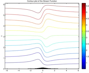
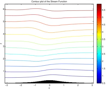
represents the “terrain following stream function” which was defined in (37). We can recover the flow field(u, w)from this function using (37) and (35). From this vector field it is easy to compute the “regular” stream functionφ (x, z). Fig-ures 1 and 2 depict the regular stream functions for the ter-rains given by (62) and (66) respectively. These figures were obtained by direct evaluation of the formulas given above.
We compare now these analytic results with the solution methodology that has been used previously in the literature as was discussed Sect. 2. First we note that this analytic so-lution requires only the direct (and simple) computation of the Hilbert transform of the terrain functionh(x). This is a straightforward procedure even if it has to be done numeri-cally. On the other hand to computeq(x)using (29) requires in general the solution of an integral equation. To do so one must use an iterative algorithm which might turn out to be un-stable or non-convergent over complex terrain. Furthermore there is the issue of applying the boundary conditions onψ
x
z
Contour plot of the Stream Function
−6 −4 −2 0 2 4 6
0 1 2 3 4 5 6
1 1.5 2 2.5 3 3.5 4 4.5 5 5.5
Fig. 1.The regular stream functionφover one hill centered atx=0 with heighth(x)=ǫh1(x)whereh1is given by Eq. (62), ǫ=0.1,
N=1,β=0,µ=0.
at the terrain. To this end the procedure discussed in Sect. 2 requires the use of the approximations that lead to (26). As a result the equation that is used to computeq(x)(Eq. 29) is also an approximate equation which will yield at best approx-imate solution for this function. On the other hand the appli-cation of the boundary conditions using the procedure dis-cussed in this section is exact and does not place constraints on the height of the terrain.
From an experimental geophysical point of view it has been a common practice to assume that the gravity wave gen-erated by a flow over terrain is of the form sin(kx+mz)(or similar) (Shutts, 1988; Jumper, 2005; Eckermann, 1999; De-wan, 1998). This has led to difficulties in the eduction of this wave from experimental data. Our results show that this form of the wave is incorrect (at least in principle). Furthermore as Fig. 2 demonstrates complex terrain can alter drastically the shape and amplitude of this wave due to interference effects. 4.2 The limiting case|h(x)|≪1,β≪1
Under these limiting conditions it is appropriate to introduce an order parameterǫso that
h(x)=ǫ h1(x) (68)
and consider a two parameter expansion of the stream func-tion inǫandβviz.
ψ (x, z)=ψ(0)(x, z)+βψ(1)(x, z)+ǫψ(2)(x, z)+O
ǫ2, β2, ǫβ
(69) The first order expansion of (51) in the parametersǫandβ
yields the following equations forψi,i=0, 1, 2.
µ2ψxx(1)+ψzz(1)+N2ψ(1)−1
2µ
2N2ψ(0) x
2
=0 (71)
µ2ψxx(2)+ψzz(2)+N2ψ(2)=1−z
H
h
N2h1+µ2
h′′1ψz(0)+ 2h′1ψxz(0)i−2h1
H ψ
(0)
zz (72)
It is easy to see that the solution to (70) subject to the the boundary conditions (49), (52) is
ψ(0)(x, z)=z. (73)
Due to this result (71) (72) simplify and it is straight forward to see that the general solution to these equations is
ψ(1)(x, z)=
Z N/µ
0
sinλz[A1(ω)cos(ωx)+B1(ω)sin(ωx)]dω+ Z N/µ
0
cosλz[C1(ω)cos(ωx)+D1(ω)sin(ωx)]dω , (74) whereµ2ω2+λ2=N2. Similarly,
ψ(2)(x, z)=
Z N/µ
0
sinλz[A2(ω)cos(ωx)+B2(ω)sin(ωx)]dω+
Z N/µ
0
cosλz[C2(ω)cos(ωx)+D2(ω)sin(ωx)]dω+
H−z
H h1(x). (75) Applying the boundary condition (52) to theψ(1)(x, z)and
ψ(2)(x, z)we infer thatC1=D1=0 and
Z N/µ
0 [
C2(ω)cos(ωx)+D2(ω)sin(ωx)]dω=−h1(x) . (76) The radiation boundary condition implies that
Z N/µ
0 [
A2(ω)cos(ωx)+B2(ω)sin(ωx)]dω=−H (h1(x)) (77) andA1=B1=0. Thus, in the present settings, the first order
contribution of theβ terms vanishes when the base stream function satisfies (49). This can be verified directly by per-forming a one parameter perturbation expansion onψviz. by lettingβ=ǫβ1and
ψ (x, z)=ψ(0)(x, z)+ǫψ(1)(x, z)+Oǫ2 (78) When the topography is given by Eq. (64) witha=1 it is easy to show using Eq. (76) thatD2=0 andC2(ω)=−e−ω.
Similarly (using Eq. 65) we obtainA2=0 andB2(ω)=−e−ω.
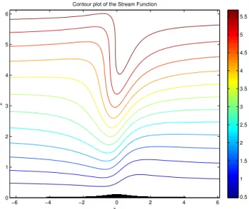
Substituting this data in Eq. (74) we can computeψ(2) by numerical integration. We observe however that these inte-grals are highly oscillatory and appropriate numerical rou-tines have to be used to evaluate them accurately. The results of these computations withµ=0.25 (re-expressed in terms of the regular stream functionφ) are shown in Fig. 3.
x
z
Contour plot of the Stream Function
−10 −5 0 5 10
0 1 2 3 4 5 6
1 1.5 2 2.5 3 3.5 4 4.5 5 5.5
Fig. 2. Same as Fig. 1 but h(x) is given by Eq. (66) with
c1=c2=c3=1 anda=1.
x
z
Contour plot of the Stream Function
−3 −2 −1 0 1 2 3
1 2 3 4 5 6
0.5 1 1.5 2 2.5 3 3.5 4 4.5 5 5.5
Fig. 3. The regular stream functionφ over one hill centered at
x=0 with heighth(x)=ǫh1(x)whereh1is given by Eq. (64) with
a=1,ǫ=0.25,N=1,β=0,µ=0.25. The computations are based on Eqs. (73) and (74).
4.3 The limiting caseβ6=0,µ=0 In this limiting case Eq. (51) becomes ∂2ψ
∂z2−GN 2
(
−ψ+β 2 "
1
G
∂ψ ∂z
2
−1 #
+z+h(x)1−z H
)
=0. (79)
sat-x
z
Contour plot of the Stream Function
−6 −4 −2 0 2 4 6
0 1 2 3 4 5 6
0.5 1 1.5 2 2.5 3 3.5 4 4.5 5 5.5
Fig. 4.The regular stream functionφover one hill centered atx=0 with heighth(x)=ǫh1(x)whereh1is given by Eq. (64) witha=1,
ǫ=0.1,α2=0.01,µ=0. The computations are based on Eqs. (82)– (87).
isfied in most practical situations). Expressingψ approxi-mately as
ψ=ψ0+α2ψ1
and substituting this expression in Eq. (61) we obtain to order zero and one in the parameterα2the following equations
∂2ψ0 ∂z2 +GN
2ψ
0=GN2
h
z+h(x)1− z
H
i
(80)
∂2ψ1 ∂z2 +GN
2ψ1
−
∂ψ
0 ∂z
2
= −G (81)
The boundary conditions onψ0,ψ1are given by Eq. (52)
atz=0 and radiation boundary conditions asz→∞.
Solving these (linear) equations forψ0andψ1we obtain
the following expressions for their solutions ψ0(x, z)=A(x)cos(νz)+B(x)sin(νz)+
h
z+h(x)1−z H
i
(82) ψ1(x, z)=C1(x)cos(νz)+C2(x)sin(νz)+f1(x, z)+f2(x, z)+f3(x) (83) where
f1(x, z)=
A2(x)−B2(x)
cos (2νz)+2A(x)B(x)sin(2νz)
6 (84)
f2(x, z)=
(H−h(x)) ((νA(x)z+B(x))cos(νz)+νB(x)zsin(νz))
H ν (85)
f3(x)=
A(x)2+B(x)2
2 (86)
where Eq. (32) was used to simplify Eq. (86).
Since V(80) is the same as V(55) it follows that
A(x)=−h(x)andB(x)is given by Eq. (61). Applying the boundary condition Eq. (52) toψ1we obtain
C1(x)=−
1 3
2A(x)2+B(x)2−1 ν
1−h(x)H
B(x) (87) Similarly the radiation boundary condition leads to
C2(y)=−H (C1(x)). For a topography described by Eq. (64) witha=1 we computedC1andC2 (analytically) and used (83) to calculate ψ1. Figure 4 displays the corresponding regular stream functionφ (x, z)whenα2=10−3.
5 Summary and conclusions
We derived in this paper a terrain following formulation of Long’s equation in which the topography is “absorbed” in the coefficients of the differential equation representing the flow rather than being part of the boundary conditions. We used this representation to solve Long’s equation analytically in some limiting cases and over complex topography. The new formulation also opens the possibility to develop analytical estimates which compare the solutions of this equation over different topographies. The analytical and numerical treat-ment of the solutions to Eq. (52) for general values ofµand
βwill be left to a subsequent publication.
From a geophysical point of view it well known that some present models for the generation of gravity waves over estimate this effect (Eckermann, 1999; Dewan, 1998; Humi, 2004b). Partially, this is due to the fact that they use oversimplified representation of the terrain. Furthermore they do not take into account the effects that are due to complex terrain (as demonstrated by our simulations). We believe that the new form of Long’s equation will make it easier to consider more realistic representations of the terrain and its effect on the generation and propagation of gravity waves.
Edited by: R. Grimshaw
Reviewed by: two anonymous referees
References
Baines, P. G.: Topographic effects in Stratified flows, Cambridge Univ. Press, New-York, 1995.
Nappo, C. J.: Atmospheric Gravity Waves, Academic Press, Boston, 2002.
Davis, K. S.: Flow of Nonuniformly Stratified Fluid of Large Depth over Topography, M.Sc. thesis in Mechanical Engineering, MIT, Cambridge, MA, 1999.
Drazin, P. G.: On the steady flow of a fluid of variable density past an obstacle, Tellus, 13, 239–251, 1961.
Drazin, P. G. and Moore D. W.: Steady two dimensional flow of fluid of variable density over an obstacle, J. Fluid. Mech., 28, 353–370, 1967.
Dubreil-Jacotin, M. L.: Sur la determination rigoureuse des ondes permanentes periodiques d’ampleur finie, J. Math. Pure. Appl., 13, 217–291, 1934.
Durran, D. R.: Two-Layer solutions to Long’s equation for verti-cally propagating mountain waves, Q. J. Roy. Meteor. Soc., 118, 415-433, 1992.
Eckermann, S. D. and Preusse, P.: Global measurements of strato-spheric mountain waves from space, Science, 286, 1534–1537, 1999.
Haagenson, P. L., Dudhia, J., Grell, G. A., and Stauffer, D. R.: The Penn State/NCAR mesoscale model(MM5) source code docu-mentation, NCAR Technical Note, NCAR/TN-392+STR, 1994. Humi, M.: On the Solution of Long’s Equation Over Terrain, Il
Nuovo Cimento C, 27, 219–229, 2004a.
Humi, M.: Estimation of Atmospheric Structure Constants from Airplane Data, J. Atmos. Ocean. Tech., 21, 495–500, 2004b. Humi, M.: On the Solution of Long’s Equation with Shear, Siam J.
Appl. Math, 66(6), 1839–1852, 2006.
Humi, M.: Density representation of Long’s equation, Nonlin. Pro-cesses Geophys., 14, 273–283, 2007,
http://www.nonlin-processes-geophys.net/14/273/2007/. Jumper, G. Y., Vernin, J., Azouit, M., and Trinquet, H.:
Compar-ison of Recent Measurements of Atmospheric Optical Turbu-lence, AIAA paper, AIAA-2005-4778, 2005.
Kar, S. K. and Turco, R. P.: Formulation of a Lateral Sponge Layer for Limited Area Shallow-Water Models and an Extension for the Vertically Stratified Case, Mon. Weather Rev., 123, 1542–1559, 1995.
Lily, D. K. and Klemp, J. B.: The effect of terrain shape on non-linear hydrostatic mountain waves, J. Fluid Mech., 95, 241–261, 1979.
Long, R. R.: Some aspects of the flow of stratified fluids I. Theoret-ical investigation, Tellus, 5, 42–57, 1953.
Long, R. R.: Some aspects of the flow of stratified fluids II. Theo-retical investigation, Tellus, 6, 97–115, 1954.
Long, R. R.: Some aspects of the flow of stratified fluids III. Con-tinuous density gradients, Tellus, 7, 341–357, 1955.
Long, R. R.: The Motion of Fluids with Density Stratification, J. Geophys. Res., 64(12), 2151–2163, 1959.
Peltier, W. R. and Clark, T. L.: Nonlinear mountain waves in two and three spatial dimensions, Q. J. Roy. Meteor. Soc., 109, 527– 548, 1983.
Shutts, G. J., Kitchen, M., and Hoare, P. H.: A large amplitude gravity wave in the lower stratosphere detected by radiosonde, Q. J. Roy. Meteor. Soc., 114, 579–594, 1988.
Shutts, G. J., Healey, P., and Mobbs, S. D.: A multiple sounding technique for the study of gravity waves, Q. J. Roy. Meteor. Soc., 120, 59–77, 1994.
Smith, R. B.: Linear theory of stratified hydrostatic flow past an isolated mountain, Tellus, 32, 348–364, 1980.
Smith, R. B.: Hydrostatic airflow over mountains, Adv. Geophys., 31, 1–41, 1989.
Yih, C.-S.: Equations governing steady two-dimensional large am-plitude motion of a stratified fluid, J. Fluid Mech., 29, 539–544, 1967.