TRANSIENT AND STEADY – STATE RESPONSES FOR THE SHIP ROLLING MOTION WITH MULTIPLE SCALES LINDSTEDT POINCARE METHOD

(1)

Academic Resources / Scientific Indexing Services / SCIPIO / JIFACTOR

TRANSIENT AND STEADY – STATE RESPONSES FOR THE SHIP ROLLING MOTION

WITH MULTIPLE SCALES LINDSTEDT POINCARE METHOD

Dumitru DELEANU1

1

Assoc. Professor PhD. Eng. General Engineering Sciences Department, Constanta Maritime University

Abstract: In order to study the dynamic behavior of ships it is imperative to take into account the inherent nonlinearity of large – amplitude motions. Of the six motions of the ship, the roll oscillation is the most critical because it can lead to the capsizing. Among the models used in the literature to simulate a rolling ship we selected in this paper that one derived by Kan and Taguchi. The governing equation of motion contains a soft cubic term in the restoring moment, a linear damping and a single harmonic excitation forcing term. Exploiting the advantages of a new perturbation technique called Multiple Scales Lindstedt Poincare method, we succeeded to obtain the transient and steady – state responses both for primary resonance and the non-resonant case. The analytical solutions provided by the new method were found to be in excellent or, at least, in decent agreement with numerical simulations, depending on the magnitude of external excitation amplitude.

Keywords: Nonlinear roll, perturbation technique, primary resonance.

INTRODUCTION

In ship motion analysis, the study of large amplitude nonlinear rolling is crucial because it is closely linked with capsizes dynamics. For such roll analysis, linear approximation is no longer valid and, as a result, obtaining closed form solutions becomes dificult or even impossible. The nonlinear effects occur mainly due the nature of restoring moment, of damping and of hydrodynamical forces and moments acting on the ship. The first ones can be approximated reasonably well by quadratic or cubic polynomial of roll angle. Realistic restoring representations, like fifth or higher-order polynomial lead to tremendously problems when the analytical route is followed [1]. The damping is usually inserted in the equation of roll motion by means of linear - quadratic or linear – cubic terms in the angular roll velocity [2, 3]. Finally, the hydrodinamic forces can be modeled as series expansions about a forward cruising speed whose coefficients can be provided by different approaches [4].

Undoubtedly, it is of interest to be able to include in the roll equation as many as possible parameters involved in a real sea, but analytical solutions are impossible in all but the simplest cases. One can resorts to numerical methods but they often give very little insight into the structure of the solutions or the effects of the various parameters embedded in the governing equation. Some useful information can, however, be obtained by considering particular cases, for example those in which damping is assumed linear, the restoring moment is represented by a third-order polynomial and the regular waves are described by a single frequency harmonic

excitation. For these simplified models, steady state responses to the external forcing can be approximated either analitically, e.g by means of harmonic balance method, or numerically, e.g. using fast Fourier transform [5-7].

Generally, the roll equations proposed in the literature are strongly non-linear, thus the classical perturbation methods including the Lindstedt Poincare and Multiple Scales are unusable [8]. To extend the range of validity of these perturbation schemes to strongly non-linear systems, researchers working in different branches of physics, engineering and applied mathemtics have developed a number of techniques [9 - 12]. Recently, Pakdemirli et al proposed a new perturbation algorithm to handle this kind of systems. Because it combines the well – known Linstedt Poincare and Multiple Scales methods, the new approach was called Multiple Scales Lindstedt Poincare method (hereafter referring as MSLP method) and applied to the free and forced damped / undamped hard Duffing oscillator. The analytical solutions provided by the new method were found to be in good agreement with numerical simulations even in the strong non-linear case [13 -15].

In this contribution, we explore the transient and steady – state solutions of the symmetric roll equation (studied in [16] and thought as a soft Duffing oscillator) and perform a comparison between the analytical solutions provided by MSLP method and numerical simulations. Our study includes both the primary resonance and the non-resonant case.

(2)

Academic Resources / Scientific Indexing Services / SCIPIO / JIFACTOR ROLL EQUATION

In this paper, the following equation, derived by Kan and Taguchi [16], is further investigated with a view to study the ship’s roll motion

M GM

W t d d t d d I

V

=     

  

      − ⋅ ⋅ + +

2

2 2

1

ϕ

ξ

ϕ

(1)

where ϕ is the roll angle, t is the time,

ϕ

_V represents the vanishing angle of stability, I is the moment of the inertia for roll, ξ the damping coefficient, W the displacement weight, GM the metacentric height, M =M₀cosΩ_et the exciting moment and Ω_e the encounter angular frequency.

Equation (1) may be transformed into the nondimensional form

t f x x x

x+ + − = Ω

• • •

cos

3

β

(2)

by means of the nondimensional quantities

0 2

0 0

0

,

, ,

ω

ϕ

ω

ξ

β

ω

ϕ

e

V V

I M f

I t t I GM W x

Ω = Ω =

= =

⋅ = =

(3)

The dots denote the order of differentiation with respect to the nondimensional time

t

. Despite of its relative simplicity, equation (2) shows a wide spectrum of qualitatively distinct types of behaviours, including steady-state solutions, jumps to resonance or period doubling cascades leading to chaos [7].

Thus, for fixed

β

and

Ω

, as forcing amplitude f is gradually increased starting with zero, the systemfirst oscillates with an increasingly amplitude and period. If f is growed further the period T – orbit bifurcates into a period 2T – orbit, then period 4T – orbit, and so on. When the external amplitude f exceeds a certain value, the oscillation amplitude grows to infinity and it is said that the vessel is capsized. Sometimes, the sequence of period doubling is missing or it is very difficult to detect numerically.

Figure 1. The growth of the oscillation amplitudes with external excitation f for

different external frequencies

Ω

Figure 1 reveals the dependence of the oscillation amplitude on the sizes of external excitation f and external frequency

Ω

.In the neighborhood of the primary resonance

Ω

≈

1

, the roll angle is dangerously close to the angle of vanishing stability even for small values of forcing f.The influence of the secondary resonance

Ω

≈

1 /

3

is also felt in Figure 1.

It was mentioned before that, for a specified set of parameters

(

β

,

Ω

)

, the system (2) evolves to a limit cycle for relatively small forcing amplitudes f or goes out to infinity for sufficiently large values of f. Figure 2 allows us to distinguish between these two different behaviors. The small black rectangles stand for a safe pair

(

Ω

,

f

)

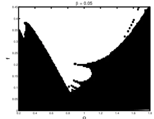
, while the white area corresonds to capsize.

Figure 2. The

(

Ω

,

f

)

parameter control plane for

β

=

0 .

05

. The black rectangles correspond

to a safe oscillation, whilst the white area is associated to a capsizing scenario

TRANSIENT AND STEADY-STATE APPROXIMATE SOLUTIONS

The aim of this section is to derive transient and steady-state approximate solutions for the roll equation (2) by using the perturbation algorithm proposed in [12] and which combine the method of Multiple scales with Linstedt – Poincare

0.2 0.4 0.6 0.8 1 1.2 1.4 1.6 1.8 0

0.05 0.1 0.15 0.2 0.25 0.3 0.35 0.4 0.45

Ω

f

β = 0.05

a = 0.1 a = 0.2

a = 0.35

a = 0.5

0.2 0.4 0.6 0.8 1 1.2 1.4 1.6 1.8 0

0.05 0.1 0.15 0.2 0.25 0.3 0.35 0.4 0.45

Ω

f

β = 0.05

(3)

Academic Resources / Scientific Indexing Services / SCIPIO / JIFACTOR technique. The new approach allows both for the

study of the transient response and for long term behavior of the analyzed system. More important, the system’s parameters do not need to be small such that the algorithm produces approximate solutions valid even for strongly nonlinear systems.

For applying the MSLP method to the equation (2), it is rewritten in the form

t f x x x

x+ + − = Ω

• •

•

cos ˆ ˆ

ˆ

2

ε

2

β

ε

α

3

ε

2 (3)

with

ε

<<1 a small parameter and

α

ˆ,

β

ˆ and fˆof O(1). According to the standard Linstedt – Poincare method, a new variable

t

ω

τ

= (4)

is introduced, where

ω

is the unknown frequency of the system. Equation (3) then becomes

τ

ω

ε

α

ε

β

ω

ε

ω

2

x

''

+

2

ˆ

x

'

+

x

−

ˆ

x

3

=

2

f

ˆ

cos

Ω

(5)

where primes denote differentiation with respect to the new time variable

τ

. Now, we introduce three independent time scales

2 , 1 , 0

, =

= n

Tn

ε

n

τ

(6)

representing the slow and fast times and expand the dependent variable x and its derivatives in power series in the small parameter

ε

(

0 1 2

)

1

(

0 1 2

)

2 2

(

0 1 2

)

0T ,T ,T x T ,T ,T x T ,T ,T x

x= +

ε

+

ε

...

2 2 1

0+ + +

=D D D

d

_ε

τ

(7)

(

2

)

...

2 ₀ ₁ 2 ₁2 ₀ ₂

2 0 2 2

+ +

=D D D D D D

d

_ε

τ

where , ₂,

2 2

i i i i

T D T D

∂ ∂ = ∂

∂

=

and

j i j i

T T D D

∂ ∂

∂

= 2

.

Thus, instead of determining the dependent variable x as a function of time

τ

, one determines it as a function of T₀,T₁, and T₂. For extend the range of validity of these perturbation expansions to the cases where the system’s parameters are not small, the square of the frequency is expanded too in power series of

ε

...

1 ₁ 2 ₂

2₌ ₊

_ε

_ω

₊

_ε

_ω

₊

ω

(8)

and the substitution

...

1=

ω

2−

ε

ω

₁−

ε

2

ω

₂− (9) is considered. Substituting equations (7) and (9) into (5) and equating coefficients of like powers of

ε

yields the following set of linear partial

differential equation which can be solved successively:

0

: 2 2₀ ₀ 2 ₀

0

_ω

_D _x ₊

_ω

_x ₌

ε

(10)

3 0 0 1 0 1 0 2 1 2 1 2 0 2

1 _ˆ

2

:

ω

D x

ω

x

ω

D D x

ω

x

α

x

ε

+ =− + −

(11)

− + + −

=

+ 2 ₀ ₁ ₁ ₁ ₁ ₂ ₀

1 2 1 2 0 2 2

2

:

ω

D x

ω

x

ω

D D x

ω

x

ω

x

ε

(

+

)

− − +

− 2 ₁

0 0 0 0

2 0 2 1

2_D ₂_D _D _x ₂_β_ˆ_ω_D _x ₃_α_ˆ_x _x

ω

0

cos

ˆ _T

f

ω

Ω

+ (12)

The first order solution of equation (10) has the form

(

T T T

)

A

(

T T

) (

iT

)

cc

x₀ ₀, ₁, ₂ = ₁, ₂ exp ₀ + (13)

where cc stands for complex conjugate of the preceeding term. Inserting (13) into (11), one obtains

(

− + −

)

⋅

=

+ x i D A A A A

x

D2₀ ₁ 2 ₁ 2 ₁ ₁ 2

2

ω

₂

ω

₃

α

_ˆ

ω

( )

iT − A

(

iT

)

+cc

⋅ 3 ₀

0 ˆ exp3

exp

α

(14)

The term containing exp

( )

iT₀ will produce a secular term which should not be part of a uniformly valid expansion. It follows that

0 ˆ

3

2 2 ₁ + ₁ − 2 =

− i

ω

D A

ω

A

α

A A (15)

In contrast to the conventional method of Multiple Scales, one has two possibilities to continue. One should first impose the condition D1A=0 and

solve (15) for

ω

₁. If the solution is a real number, then one continues the algorithm by searching for

1

x . If not, one selects

ω

₁=0 and solve (15) for

.

1A

D Here, the condition D1A=0 leads to the

real value

A

α

ω

₁

=

3 ˆ

(16)

Additionally, D1A=0 means that A=A

( )

T2 .

Now, one can determine the second order approximate solution

x

₁ from (12)

(

T T T

)

A

(

iT

)

cc

x = ₂ 0 +

3 2

1 0

1 exp3

8 ˆ ,

,

ω α

(17)

The equation (12) for the third order of approximation contains into the right term the

excitation term

f

ˆ

cos

T

₀

ω

Ω

. It could be or not part

of the condition that prevent the appearence of the secular terms at this level of approximation. In the following we concentrate on the non-resonant case, where the excitation frequency

Ω

is not so

(4)

Academic Resources / Scientific Indexing Services / SCIPIO / JIFACTOR close to the oscillation frequency ω, as well as on

resonant case

ω

≈Ω. Non-resonant case

Introducing (13) and (17) into (12), the secular terms will vanish if and only if

0 8 ˆ 3 ˆ 2

2 ₂ 3 2

2 2

2

2 ₊ ₋ ₋ ₌

− i D A A iA A A

ω

α

ω

β

ω

(18)

This time, the selection D₂A=0 yields a complex value for

ω

₂, without any physical meaning. The other way to continue,

ω

₂=0, together with the polar form

( )

2

( )

2

exp

(

( )

2

)

2

1 T

i

T

a

T

A

=

γ

(19)

permit us to obtain the differential equations

4 4 2 2 2 256 ˆ 3 , ˆ a D a A D

ω

α

γ

ω

β

₌ −

= (20)

But

ε

γ

τ

γ

ε

τ

2 2 2 2 , D d d a D d a

d ₌ ₌

and

τ

=

ω

t , so

we get immediately the amplitude and phase modulation equations 4 3 2 256 3 , a a a

ω

α

γ

β

= − = • • (21)

These equations describe the transient behavior towards the steady-state solution. The three order approximation for the solution of equation (3) is now obtained from

(

)

(

)

(

+

)

+

=

+ 5 ₀

0 4 4 2 2 2 2

0 3 exp3 exp5

8 ˆ T i A T i A A x x D ω α cc T i f +       Ω

+ exp 0

2 ˆ

ω (22)

It results that

(

)

(

)

(

+

)

+

−

= 5 ₀

0 4

4 2

2 3 exp3 exp5

64 ˆ T i A T i A A x

ω

α

(

f

)

i T +cc

     Ω Ω −

+ ₂ ₂ 0

2 exp 2 ˆ

ω

(23)

As a general conclusion, the non-resonant solution of roll equation (2) can be expressed as

(

+

)

−

(

+

)

−

=

ω

γ

ω

γ

ω

t a t

a t

x cos3

32 cos ) ( ₂ 3 (24)

(

)

(

)

(

+ + +

)

+

−

ω

γ

ω

γ

ω

t t

a 5 cos 3 cos 3 2048 4 5 t f _Ω Ω −

+ ₂ ₂cos

2

ω

with a and γ given by (21) and

4 3 1 2 a − =

ω

(25)

A careful consideration of modulation equations (21) shows that a→0 as t→∞, so the steady-state behaviour of system (2) in non-resonant conditions is governed by

( )

t f t

x Ω

Ω −

= cos

1 2 (26)

Resonant case

ω

≈Ω

The fact that excitation frequency Ωis close to the oscillation frequency

ω

could be written as

(

ε

σ

)

ω

2

1+

=

Ω (27)

with σ =O(1) a detuning parameter. Because

(

0 2

)

( ) (

0 2

)

0

exp

2

1 cos

cos

T

σ

T

i

T

i

σ

T

ω

=

+

=

Ω

the secular term in (12)will vanish if and only if

0 2 ˆ 8 ˆ 3 ˆ 2

2 3 2 2

2 2 2

2

2 ₊ ₋ ₋ ₊ ₌

− i T

e f A A A i A A D i σ ω α ω β ω ω

The selection D₂A=0 provides a complex

ω

₂, so we choose

ω

2=0and solve the previous

equation for D₂A. Replacing the polar form (19) and separating the real and imaginary parts, we get the differential system of equations in a and γ

(

σ

γ

)

ω

β

₊ ₋

−

= 2 2

2 sin 2 ˆ ˆ T f a a D (28)

(

σ

γ

)

ω

α

γ

= 4− ₂ ₂−

4 2 2 cos 2 ˆ 256 ˆ 3 T a f a D (29)

Returning to the time t in the same way as in the non-resonant case, the amplitude and phase modulation equations are written as follows

δ

ω

β

sin 2 f a a=− +

• (30)

δ

ω

γ

cos 2 256 3 3 4 a f a ₊ − − Ω = • (31)

where the phase

δ

is defined as

δ

=

σ

T

₂

−

γ

. These equations describe the transient behavior towards the steady-state solutions. The later ones

are obtained for = =0

• •

δ

(5)

Academic Resources / Scientific Indexing Services / SCIPIO / JIFACTOR where the frequency

ω

of the system is given by

(25). It could be solved grafically to yielda=a

( )

Ω . Finally, after eliminating the secular term, the equation (12) reduces to

(

)

(

)

(

A A iT A iT

)

cc

x x

D + = ₄ 4 ₀ + 5 ₀ +

2 2 2 2

0 3 exp3 exp5

8 ˆ

ω α

and has the solution

(

)

(

)

(

A A iT A iT

)

cc

x =− 4 ₀ + 5 ₀ +

4 2

2 3 exp3 exp5

64 ˆ

ω

α

(33) From (7), (13), (17) and (33), one finds that the approximate solution of (2) to O

( )

ε

3 can be expressed as

(

Ω −

)

−

(

Ω −

)

−

=

δ

ω

δ

a t

t a t

x cos3

32 cos

)

( ₂

3

(34)

(

)

(

)

(

δ

)

ω

Ω − + Ω −

− a 3cos3 t cos5 t

2048 4

5

The solution (34) is valid both for the transient period and for the steady-state one. The amplitude a and the phase

δ

yield from the modulation equations (30) and (31).

NUMERICAL RESULTS

In this section we performed a comparison between the analytical solutions (24) and (34) and the numerical ones to check the MSLP method’s efficiency. For computations and plots, Matlab package has been used.

Throughout this part the fixed values

ε

=0.1,

5 . 2

ˆ₌

β

and

α

ˆ =10 have been selected. It results that for obtaining an equation with a weak nonlinearity, therefore solvable with perturbation techniques, we encroached the preordered range for

α

ˆ. We started with non-resonant case and then we continued with the primary resonance

1

≈

Ω .

Non-resonant case

Equation (2) has been numerically integrated by use of a fourth order Runge – Kutta – Gill procedure with constant step, starting with initial

conditions (0),

( ) (

0 = 0.5,0.1

)

  



 •

x

x , and for a time

interval equal to 100 cycles of forcing (considered enough large for the transients to die out). The range for external frequency was selected to be

[

0 .

2 ,

1 .

8 ]

∈

Ω

. The excitation amplitude fˆ has been gradually increased from small values, within the preordered range, till large enough values. The oscillation amplitude recorded in the last few cycles was kept and plotted versus the

same quantity given by the analytical solution (24). The findings are displayed in Figure 3. Numerical results are labeled by red asterisks on the graphs while the results provided by MSLP method are associated to grey small points. For fˆ≤10, MSLP solutions are in excellent agreement with those obtained by Runge – Kutta – Gill method, for the entire domain of external frequencies excepting a small neighborhood of

1

=

Ω . If fˆ exceeds 10, the MSLP solutions are still in pretty good agreement with numerical ones, especially for Ω>1.2. For this level of forcing, the secondary resonance Ω≈1/3 becomes „visible” and make necessary another approximate solutions. A last thing to observe is what happens in the proximity of Ω=1. Here, the numerical scheme provides unbounded solutions and this explains the absence of the asterisks above a certain value of fˆ. MSLP method gives unphysical solutions (see also Figure 2).

0.2 0.4 0.6 0.8 1 1.2 1.4 1.6 1.8 0

0.05 0.1 0.15 0.2 0.25 0.3 0.35 0.4 0.45 0.5

Ω

aM

S

L

P

, a

N

u

m

( a )

Num MSLP

0.2 0.4 0.6 0.8 1 1.2 1.4 1.6 1.8 0

0.1 0.2 0.3 0.4 0.5 0.6 0.7 0.8 0.9 1

Ω

aM

S

L

P

, a

N

u

m

( b )

Num MSLP

0.2 0.4 0.6 0.8 1 1.2 1.4 1.6 1.8 0

0.1 0.2 0.3 0.4 0.5 0.6 0.7 0.8 0.9 1

Ω

aM

S

L

P

, a

N

u

m

( c )

Num MSLP

(6)

Figure 3. The comparison between Ω−a

curvesobtained withMSLP method and Runge – Kutta - Gill method. The asterisks stand for

numerical solution.

a) fˆ =2; b) fˆ=5; c) fˆ=10; d) fˆ=20.

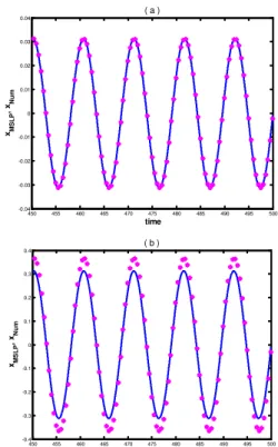
The previous observations are confirmed by the plots in Figure 4, where the numerical solution (red asterisks) is contrasted with MSLP solution (continuous blue line) for Ω=0.6 and different

fˆ

Figure 4. The comparison between time series solutions

x

=

x

( )

t

obtained withMSLP method

and Runge – Kutta – Gill method. The asterisks stand for numerical solution.a)

2

ˆ ₌

f ; b) fˆ=20.

Resonant case

ω

≈Ω

The steps of the same algorithm were followed for primary resonance. In this range of external frequencies, the excitation amplitude fˆrequired for the system (2) to have unbounded solutions does not exceed values of order 7 to 10 (see Figure 2). In Figure 5, the frequency – amplitude curves Ω−a given by (34) are compared with those yielded by numerical integration. The range for Ω was thought to be [0.5, 1.5]. It is toolarge for our purpose, but we wanted to see how behaves the solution (34) away from the area of interest, Ω≈1From the plots in Figure 5, it is obvious that for a weak excitation, fˆ≤5, MSLP and numerical solutions match very well, especially for

Ω

∈

[

1 ,

1 .

2 ]

.

The agreement

continues to be pretty well in the range fˆ∈

[

5,10

]

, but only for those frequencies Ω for which one has bounded solutions.

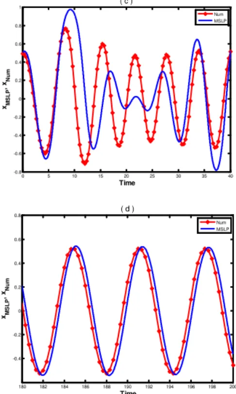
For fˆvalues selected without a flagrant order violation, the MSLP solution (34) describes both the transient and the steady-state behaviors, as proven by the first two panels of Figure 6.

As excitation amplitude overcomes significantly the preordered range fˆ=O(1), then equations (30) and (31) cease to describe correctly at least the transient state (see the last two panels of Figure 6).

0.2 0.4 0.6 0.8 1 1.2 1.4 1.6 1.8 0

0.1 0.2 0.3 0.4 0.5 0.6 0.7 0.8 0.9 1

Ω

aM

S

L

P

, a

N

u

m

( d )

Num MSLP

450 455 460 465 470 475 480 485 490 495 500 -0.04

-0.03 -0.02 -0.01 0 0.01 0.02 0.03 0.04

time

xM

S

L

P

, x

N

u

m

( a )

450 455 460 465 470 475 480 485 490 495 500 -0.4

-0.3 -0.2 -0.1 0 0.1 0.2 0.3 0.4

time

xM

S

L

P

, x

N

u

m

( b )

0.5 0.6 0.7 0.8 0.9 1 1.1 1.2 1.3 1.4 1.5 0

0.05 0.1 0.15 0.2 0.25 0.3 0.35 0.4 0.45

Ω

aM

S

L

P

, a

N

u

m

( a )

Num MSLP

0.5 0.6 0.7 0.8 0.9 1 1.1 1.2 1.3 1.4 1.5 0

0.1 0.2 0.3 0.4 0.5 0.6 0.7

Ω

aM

S

L

P

, a

N

u

m

( b )

Num MSLP

(7)

Figure 5. The comparison between Ω−a

curvesobtained withMSLP method and Runge – Kutta - Gill method. The asterisks stand for

numerical solution. a) fˆ =2; b) fˆ=5; c) fˆ =10.

Figure 6. The comparison between time series solutions

x

=

x

( )

t

obtained withMSLP method

and Runge – Kutta – Gill method. The asterisks stand for numerical solution.a)

2

ˆ₌

f (transient state); b) fˆ=2(steady – state); c) fˆ=12(transient state);d) fˆ=12

(steady – state).

CONCLUSIONS

In the paper, the symmetric roll equation proposed by Kan and Taguchi for the capsizing of a ship in quartering seas was analitically investigated by means of a perturbation technique which combine the classical Multiple Scales and Lindstedt-Poincare methods.

To this aim, the moderate nonlinear roll equation was transformed into an apparently weakly nonlinear equation and the above-mentioned procedure was applied for giving the transient and steady-state responses both for the primary resonance and the non-renonant case.

The comparison between the numerical solution provided by an ODEs integrator and their analytical counterpart derived in the paper shows an excellent agreement every time the system parameters were selected without a flagrant violation of the order’s magnitude. The two solutions match acceptable well for the long-term behavior even some of the parameters exceed the order to a certain extent, but notable differences appear for the transition period towards the steady-state. For large external excitation amplitudes, the numerical scheme ceases to provide bounded solutions (the capsizing scenario) while the perturbation technique yields unphysical solutions

0.5 0.6 0.7 0.8 0.9 1 1.1 1.2 1.3 1.4 1.5 0

0.1 0.2 0.3 0.4 0.5 0.6 0.7 0.8

Ω

aM

S

L

P

, a

N

u

m

( c )

Num MSLP

0 10 20 30 40 50 60 70 80

-0.4 -0.2 0 0.2 0.4 0.6

Time

xM

S

L

P

, x

N

u

m

( a )

Num MSLP

150 155 160 165 170 175 180 185 190 195 200 -0.4

-0.3 -0.2 -0.1 0 0.1 0.2 0.3 0.4 0.5

Time

xM

S

L

P

, x

N

u

m

( b )

Num MSLP

0 5 10 15 20 25 30 35 40

-0.8 -0.6 -0.4 -0.2 0 0.2 0.4 0.6 0.8 1

Time

xM

S

L

P

, x

N

u

m

( c )

Num MSLP

180 182 184 186 188 190 192 194 196 198 200 -0.4

-0.2 0 0.2 0.4 0.6 0.8

Time

xM

S

L

P

, x

N

u

m

( d )

Num MSLP

(8)

Academic Resources / Scientific Indexing Services / SCIPIO / JIFACTOR BIBLIOGRAPHY

[1] M.A.S. Neves, C.A. Rodriguez, Influence of non-linearities on the limits of stability of ships rolling in headseas, Ocean Engineering, 34 (11-12), p. 1618 – 1630, 2007.

[2] D.W. Bass, M.R. Haddara, Nonlinear models of ship roll damping, International Shipbuilding Progress, 35, p. 5 – 24, 1988.

[3] A. Cardo, A. Francescutto, R. Nabergoj, On damping models in free and forced rolling motion, Ocean Engineering, 9 (2), p. 171 – 179, 1982.

[4] M.A. Abkowitz, Measurements of hydrodynamic characteristics from ship maneuvering trials by systemidentification, Transactions of the Society of Architects and Marine Engineering, 88, p. 283 – 318, 1981.

[5] D. Deleanu, Comparative approximate studies on the ship’s rolling motion, Journal of Marine Technology and Environment, 1, p. 29 – 35, 2015.

[6] D. Deleanu, On a geometric approach of safe basin’s fractal erosion. Application to the symmetric capsizeproblem, Constanta Maritime University Annals, 22, p. 121 – 126, 2015.

[7] J.M.T. Thompson, Chaotic phenomena triggering the escape from a potential well, Proc. Royal Society London, A 421, p. 195 – 225, 1989.

[8] A.H. Nayfeh, Introduction to Perturbation Techniques, John Wiley and Sons, New York, 1981.

[9] J.H. He, Modified Lindstedt Poincare methods for some strongly nonlinear oscillations. Part I: expansion of a constant; Part II: a new transformation, International Journal of Non-Linear Mechanics, 37, 309 – 320, 2002.

[10] J.H. He, Some asymptotic methods for strongly nonlinear equations, International Journal of Modern Physics, B 20, p. 1141 – 1199, 2006.

[11] H. Hu, Z.G. Xiong, Comparison of two Lindstedt – Poincare type perturbation methods, Journal of Sound and Vibration, 278, p. 437 – 444, 2004.

[12] V. Marinca, N. Herisanu, A modified iteration perturbation method for some nonlinear oscillation problems, Acta Mechanica, 184, p. 239 – 242, 2006.

[13] M. Pakdemirli, M.M.F. Karahan, H. Boyaci, A new perturbation algorithm with better convergence properties: Multiple Scales Lindstedt Poincare method, Mathematical and Computational Applications, 14, p. 31 – 44, 2009.

[14] M. Pakdemirli, M.M.F. Karahan, A new perturbation solution for systems with strong quadratic and cubicnonlinearities, Mathematical Methods in the Applied Sciences, 33, p. 704 – 712, 2010.

[15] M. Pakdemirli, M.M.F. Karahan, H. Boyaci, Forced vibrations of strongly nonlinear systems with MultipleScales Linstedt Poincare method, Mathematical and Computational Applications, 16 (4), p. 879 – 889, 2011.

[16] M. Kan, H. Taguchi, Capsizing of a ship in quartering seas, J. Soc. Naval Architects Japan, 171, p. 229 – 244, 1992.