Abstract—This paper describes a new approach in using multi-objective evolutionary algorithms in evolving the neural network that acts as a controller for the phototaxis and radio frequency localization behaviors of a virtual Khepera robot simulated in a 3D, physics-based environment. The Pareto-frontier Differential Evolution (PDE) algorithm is utilized to generate the Pareto optimal sets through a 3-layer feed-forward artificial neural network that optimize the conflicting objectives of robot behavior and network complexity, where the two different types of robot behaviors are phototaxis and RF-localization, respectively. Thus, there are two fitness functions proposed in this study. The testing results showed the robot was able to track the light source and also home-in towards the RF-signal source successfully. Furthermore, three additional testing results have been incorporated from the robustness perspective: different robot localizations, inclusion of two obstacles, and moving signal source experiments, respectively. The testing results also showed that the robot was robust to these different environments used during the testing phases.Hence, the results demonstrated that the utilization of the evolutionary multi-objective approach in evolutionary robotics can be practically used to generate controllers for phototaxis and RF-localization behaviors in autonomous mobile robots.
Index Terms—Artificial Neural Networks (ANNs), Evolutionary Computation (EC), Evolutionary Multi-objective Optimization (EMO), Evolutionary Robotics (ER).
I. INTRODUCTION
Evolutionary Robotics (ER) is a methodology to develop a suitable control system for autonomous robots with minimal or without human intervention through evolutionary computation as well as to adapt itself to partially unknown or dynamic environments [1]-[3]. In other words, ER is defined as the synthesis of autonomous robots using artificial evolutionary methods [4], [5]. ER is mainly seen as a strategy to develop more complex robot controllers [1], [6]. Algorithms in ER frequently operate on a population of candidate controllers, initially selected from some random distributions [7], [8]. The evolutionary processes involve a set of operators, namely selection, crossover, mutation and other
Manuscript received June 15, 2008. This research work is funded under the ScienceFund project SCF0002-ICT-2006 granted by the Ministry of Science, Technology and Innovation, Malaysia.
Chin Kim On is with the School of Engineering and Information Technology, Locked Bag No: 2073, 88999 Kota Kinabalu, Universiti Malaysia Sabah, Sabah, Malaysia (Tel: 6088-320000 ext: 3305; fax: 6088-320029; email: [email protected]).
Jason Teo is with the School of Engineering and Information Technology, Locked Bag No: 2073, 88999 Kota Kinabalu, Universiti Malaysia Sabah, Sabah, Malaysia (email: [email protected]).
genetic algorithms (GAs) operators [9], [10]. Using different approaches of evolution, for example Genetic Algorithms, Genetic Programming and Co-evolution, researchers work for algorithms that are able to train the robots to perform their tasks without any external supervision or help.
A number of studies have already been successfully conducted in ER for phototaxis, phonotaxis and obstacle avoidance tasks [1], [4], [6], [10]-[12]. In previous studies related to phototaxis tasks, the researchers used a fixed amount of hidden neurons in the neural network or just a two-layer neural network for their robot’s task [1]-[7], [13]-[17]. They have not emphasized on the relationship between the robot’s behavior and its corresponding hidden neurons. Additionally, to the best of our knowledge, there have not been any studies conducted yet in using evolutionary multi-objective algorithms in evolving the robot controllers for phototaxis behavior. Also, the literature showed that other researchers have successfully synthesized some fitness functions to evolve the robots for the required behaviors [1], [6], [10]. However, the fitness functions used can be further improved or augmented in order to increase the robot’s ability in completing more complex tasks [18]. In addition, research regarding radio frequency (RF) signal localization has yet to be studied in ER. The RF-signal is defined as a radio frequency signal (abbreviated RF, rf, or r.f.) [19]-[21]. It is a term that refers to an alternating current having characteristics such that if the current is an input to an antenna, an electromagnetic field is generated that is suitable for wireless broadcasting and/or communications [19]-[21]. The RF-signal source has provided the capability for improvements in tracking, search and rescue efforts. As such, robots that are evolved with RF-localization behaviors may potentially serve as an ideal SAR assistant [19]-[21].
Previous studies of evolution mainly focused on achieving a single objective and they were unable to explicitly trade-off in terms of their different objectives when there is problem that involves more than one objective [22]-[25]. With respect to the other ANN studies, the EMO application is advantageous compared to some conventional algorithms, such as backpropagation, conventional GAs, and Kohonen SOM network [6]-[9]. For example, the number of hidden neurons used in multiple layer perceptrons (MLP) and the number of cluster centers in Kohonen’s SOM network need to be determined before training [6]-[9]. Meanwhile, the traditional learning methods for ANNs such as backpropagation usually suffer from the inability to escape from local minima due to their use of gradient information [4]. In addition, EMOs are able to solve two or more objectives in a single evolutionary process compared to conventional GAs
Artificial Neural Controller Synthesis in
Autonomous Mobile Cognition
Chin Kim On,
Student Member, IEEE, IAENG
and Jason Teo,
Member, IEEE, ACM
[4]. An EMO emphasizes on the generation of Pareto optimal set of solutions that explicitly trade-offs between more than one conflicting and different optimization objectives. In previous work done by Teo [4], it was proven that the multi-objective evolutionary algorithm was able to discover reasonably good solutions with less computational cost if compared to a single-objective EA, a weighted-sum EMO, and a hand-tuned EMO algorithm for simulated legged robots.
In this study, the Pareto Differential Evolution (PDE) algorithm is used as the primary evolutionary optimization algorithm [8], [22]-[23]. There are two separate behaviors to be optimized: phototaxis and RF-localization behavior respectively. Thus, there are two experiments conducted and discussed in this paper. Firstly, there are two distinct objectives to be optimized for the phototaxis behavior: (1) maximizing the robot’s phototaxis behavior and (2) minimizing the complexity of the neural controller in terms of the number of hidden units used. There are also two distinct objectives to be optimized for the RF-localization behavior: (1) maximizing the robot’s RF-localization behavior and (2) minimizing the neural network complexity, similar to the first experiment. Thus, a multi-objective approach [26]-[28], which combines the Differential Evolution algorithm and Pareto multi-objective concepts is used, namely the PDE-EMO algorithm [4], [5], [17], [25]. The elitist PDE-EMO is used to generate a Pareto optimal set of ANNs that acts as a robot controller. Typically, an elitist algorithm is used to avoid losing good solutions during the EMO optimization process. In the study of [25]-[30], it was clearly shown elitism helps in achieving better convergence in EMOs. Thus, this study’s main objective is to verify the performance and the ability of the generated robot controllers using the PDE-EMO algorithm in the ER study. Furthermore, the optimum solutions obtained through the RF-localization study are then utilized for robustness testing purposes. It is not surprising if the generated controllers from the phototaxis behaviors are robust to different environments used during testing phases. The light’s intensity is able to assist the robot to home in towards the light source easily since it is visible from the entire environment. Nevertheless, such an advantage does not exist in the RF-localization behavior. In RF-localization behavior, the receiver located on the top of the robot can only detect the signal if it is within the range of emitter source; otherwise no signal is detected. Thus, different experimental setup used during testing phases may affect the robot’s tracking, exploring, and homing performances.
There are three extra tests conducted for the robustness: different robot localizations, inclusion of two obstacles, and moving signal source experiments. Firstly, the robot’s robustness is tested by positioning the robot at five different locations but in the same environment as that used during evolution as well as testing phases: top left corner, top right corner, middle of the ground, bottom left corner and bottom right corner of the testing environment, respectively. We expect the robots to be capable of exploring and homing in towards the signal source even when the robots are localized at different positions during testing phases.
Furthermore, two obstacles were included in the testing environment to purposely block the most common paths for the robot used in homing towards the signal source. The robot’s robustness is tested by moving both of the obstacles
some distance to the left, right, top, and bottom. In our experiment, the robot must successfully find another way to track the signal source and home towards the signal source as fast as possible even when the common paths used were blocked by the obstacles. In addition, the robot must also be able to home in towards the signal source even when the testing and evolution environments are different with respect to the positioning of the obstacles.
Lastly, the robot's tracking ability and robustness are tested by moving the RF-signal source to five different positions in the environment, 60 seconds being permitted for each of the different position. The RF-signal source is located at the top left corner, top right corner, bottom right corner, bottom left corner, and center of the ground, respectively 60 seconds for each position. In our experiment, the robot must successfully track the signal source as fast as possible even the RF-signal source is moved to different position at every 60 seconds. Furthermore, the robot must also be able to home in towards the signal source even when the testing and evolution environments are different with respect to the positioning of the RF-signal source.
The remainder of this paper is organized as follows. In Sections II and III, the ANNs and methodology used in evolving the robot controllers are discussed. In Section IV, we give an explanation of the experimental setup used for both the phototaxis and RF-localization behaviors. Furthermore, the fitness functions used are presented in Section V. In Sections VI and VII, the evolution and testing results are presented, respectively. Then, the robustness tests are further discussed in Section VIII. Finally, Section IX summarizes the conclusion and proposed future work arising from this study.
II. ARTIFICIAL NEURAL NETWORKS
Neural networks are widely used for classification, approximation, prediction, and control problems. Based on biological analogies, neural networks try to emulate the human brain’s ability to learn from examples, learn from incomplete data and especially to generalize concepts. A neural network is composed of a set of nodes connected by weights. The nodes are partitioned into three layers namely input layer, hidden layer and output layer [4], [5]. The neural network architecture used in this study is a simple 3-layer feed-forward ANN, where the data flows in a single direction, which are from the input layer through to the hidden layer and finally to the output layer. Each path will be assigned a weight to strengthen or weaken the input value to get a net input. Each node will take the weighted sum of inputs from previous layer’s nodes and apply them to an activation function before delivering the output to the next node.
In this paper, the experiments are conducted with a Khepera robot. The Khepera robot is integrated with 8 light sensors and 2 wheels during the phototaxis simulation while the robot is integrated with 8 infrared distance sensors, 2 wheels and 1 extra RF receiver during the RF-localization simulation. The chromosome in this experiment is a class that consists of a matrix of real numbers that represents the weights used in the ANN controller. The binary number for the hidden layer represents a switch to turn a hidden unit on or off. Fig. 1 below depicts the morphogenesis of the chromosome into the ANN robot controller architecture.
are passed to the ANN as input. There are a maximum of 15 hidden neurons permitted during the optimization processes. All of the hidden nodes are included in the hidden layer but are switched off (0) or on (1) randomly to evolve the number of active hidden nodes. The ANN’s outputs determine robot’s speed, left wheel and right wheel respectively.
In the RF-localization evolution, the infrared distance sensors and RF receiver are presented as input neurons to the ANN while the speed of the robot’s wheels represents the output neurons from the ANN. Similar to the phototaxis behavior’s evolutionary optimization, the maximum number of hidden neurons permitted in evolving the RF-localization controllers is 15 but are switched on and off randomly to evolve the number of active hidden nodes.
III. THE PDE-EMOALGORITHM
This paper investigates a multi-objective problem which solves two objectives simultaneously: (1) maximize the light following behavior for the phototaxis task and maximize the RF signal source homing behavior for RF-localization, respectively whilst (2) minimize the number of hidden units used in the neural controller. The Pareto-front thus represents a set of networks with different numbers of hidden units and different numbers of tracking and homing behaviors. The elements of the binary vector are assigned the value 1 with a probability of 0.5 (P(X=0.5) to give the hidden layer a 50% probability of either switching on or off a hidden unit in the vector of hidden units which is being evolved) based on a randomly generated number according to a uniform distribution between [0, 1]; otherwise a value of 0 is assigned. The elitist PDE algorithm used in evolving the robot controller is presented next.
1.0 Begin.
2.0 Generate random initial population of potential chromosomes. The elements of the weight matrix are assigned random values according to a Gaussian distribution N(0, 1). The elements of the binary vector ρ are assigned the value 1 with probability 0.5 based on a random generated number according to a uniform distribution between [0, 1]; 0 value otherwise.
3.0 Loop
3.1 Evaluate the individuals or solutions in the population and label as parents those that are non-dominated according to the two objectives: maximizing the robot’s behavior and minimizing the number of hidden neurons.
3.2 If the number of non-dominated individuals (a solution is considered as non-dominated if it is optimal in at least one objective) is less than three, repeat the 3.2.1 and 3.2.2 steps until the number of non-dominated individuals is greater than or equal to three (since the Differential Evolution algorithm requires at least three parents to generate an offspring via crossover). If insufficient solutions are retained from the first layer, then 3.2.1 and 3.2.2 steps have to be repeated for the second and subsequent layers of the non-dominated solutions.
3.2.1Find a non-dominated solution among those who are not labeled in the second layer of the non-dominated results.
3.2.2Label the solution(s) found as the non-dominated points.
4.0 Delete only dominated solutions from the population and retain the non-dominated solutions (elitist concept). 4.1 Loop
4.1.1Select at random an individual as the main parent α1, and other two parents α2, α3 as supporting parents.
4.1.2Crossover with some uniform (0,1) probability, do
)
)(
1
,
0
(
2 31
ih ih ihchild
ih
N
if
(
1
(
0
,
1
)(
2
3))
0
.
5
hh
h
N
;1
child h
;
hchild
0
Otherwise;Otherwise; 1
ih child ih
1
h child h
And with some uniform (0,1) probability, do
)
)(
1
,
0
(
2 31
ho ho hochild
ho
N
Otherwise; 1
ho child ho
4.1.3Mutate with some uniform (0,1) probability, do
)
_
,
0
(
mutation
rate
N
child ih child
ih
)
_
,
0
(
mutation
rate
N
child ho child
ho
if
hchild
0
1
child h
; 0 otherwise4.2 Repeat for all of the deleted solutions.
5.0 Repeat until maximum number of generations is reached. 6.0 End
In general, DE differs from a conventional GA in a number of ways. The number of vectors used for the crossover operation is the main difference. In DE, three vectors are utilized for the crossover, where one of the selected Fig 1. The representation used for the chromosome.
non-dominated parents serves as the base vector to which the differences between the other two parents’ vectors are added to form the trial vector. Then, the new trial vector will replace the randomly selected base vector only if it is better [25]. The vector selection method used in the algorithm for high behavior’s fitness score with less number of hidden neurons used during the optimization processes is able to maximize the robot behavior whilst minimize the neural network complexity in the evolution process.
IV. EXPERIMENTAL SETUP
A physics-based simulator namely WEBOTS is used in the experiment for simulating the Khepera robot behavior. The standardized virtual Khepera robot model is ready for used in the simulator. The WEBOTS simulator has an advantage in that random noise as occurring in real Khepera robots is included for all the distance sensors and robot wheels [30]. Thus, the robot may have slightly different responses even if the same controller and inputs from the environment are used. This is highly advantageous since the simulation results represent the real-life functioning of a physical robot and more importantly, the evolved controllers are directly transferable to a real physical robot.
Both of the phototaxis and RF-localization experiments utilized similar evolution and testing environment. The evolutions are conducted to evolve the robot controllers for the required behaviors. The tests are conducted purposely to verify the performances of the generated/evolved controllers as well as the effectiveness and ability of the PDE-EMO algorithm used in producing the required offspring and the ability in reducing the ANNs complexity in terms of number of hidden neurons involved during optimization processes.
A. Phototaxis Experimental Setup
A Khepera robot is positioned randomly in a simulation environment that was created using WEBOTS in a 1m2 floor surrounded by walls, where there is a static light source located at one corner of the environment. The robot has to learn to move towards the light source during the evolution process. The robot is expected to be able to sense the light intensity with its light sensors, and returns a lower value when a higher light intensity is detected, which indicates the robot is approaching the light source. Fig. 2 below depicts the simulation environment used during the phototaxis evolution optimization processes.
Fig 2. Environment used for phototaxis behavior.
B. RF-Localization Experiment Setup
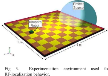
A Khepera robot is located on the ground with four walls. The area of the ground covered is 1m2. The Khepera robot is located somewhere on the ground and facing the nearest wall. A receiver is located on top of the Khepera robot. It acts as a device which can receive any signal that comes from an RF emitter. An emitter is a modeled device that can send RF signals at every time step. The receiver can only detect the signal if it is within the range of emitter source; otherwise no signal is detected. The emitter source used is a radio type with buffer size 4096 and byte size 8 with radius 0.3 meter range. It is located as a static emitter near to the center of one of the walls and to the back of the Khepera robot. The experimental setup used for RF-localization behavior is depicted in Fig. 3.
Fig 3. Experimentation environment used for RF-localization behavior.
C. Parameter Settings
Both of the phototaxis and RF-localization behavior simulations utilized similar parameter settings during the evolutionary optimization processes. The maximum number of hidden units permitted in evolving the ANN was fixed at 15 nodes. The optimum solutions with the least possible number of hidden neurons used will be automatically generated with the utilization of the PDE-EMO algorithm. The success rate for the robot in terms of moving towards the light/signal source is optimal if the number of generations is set to at least 100. However, it is not necessary to evolve the robot with more than 100 generations, because the robot is already able to successfully evolve behaviors that orient towards the light/signal source well within 100 generations. For the same reason, 60 seconds is sufficient for the simulated task duration, because the robot is also able to successfully evolve behaviors that orient towards the signal source well within 60 seconds. The previous studies [31], [32] clearly showed that the optimum solutions could be generated with 70% crossover rate and 1% mutation rate, respectively. Table 1 presents the parameters used in evolving the robots’ controllers.
D. Robustness Tests Setup
TABLE1
PARAMETERS USED FOR PHOTOTAXIS &RF-LOCALIZATION SIMULATIONS
Descriptions Parameters
Number of Generation 100
Population Size 30
Simulation Time Steps 60s
Crossover Rate 70%
Mutation Rate 1%
Number of Hidden Neurons 15 Number of Repeated Simulations 10
Algorithm Used Elitist PDE-EMO
Random Noise Feature Activated
environment as that used for evolution but using five different initialization positions, purposely for robustness tests: top left, top right, middle, bottom left, and bottom right of the testing environment; abbreviated as TL (top left of the top view), TR (top right of the top view), BL (bottom left of the top view), BR (bottom right of the top view), and CO (center of the top view). Fig. 4 depicts the discussed environment used.
(a) (b) (c)
(d) (e)
Fig 4. Testing setup used. (a) = TL testing environment, (b) = TR testing environment, (c) = BL testing environment, (d) = BR testing environment, and (e) = CO testing environment.
Furthermore, there are two obstacles included in the testing environment in order to increase the complexity of the environment used. Both of the obstacles are purposely positioned to block the most common paths used for the robot to home in towards the signal source. Fig. 5 depicts the experimental setup used in the testing environment.
Fig. 5. Experimental setup used for two obstacles inclusion. A top-down view shows the two obstacles (rectangular objects) that blocks the most common paths used by the robot;
semi-sphere represents the RF-signal source area whilst the sphere object represents the Khepera robot facing the nearest wall.
Furthermore, the obstacles were moved slightly along four different axes: left, right, upwards, and downwards, respectively 0.05m for each axis, which are Z+0.05 (move towards left), Z-0.05 (move towards right), X+0.05 (move upwards), and X-0.05 (move downwards). Fig. 6 depicts the testing environments used for the robustness tests.
(a) (b) (c)
(d) (e)
Fig 6. Testing setup used. (a) = original environment, (b) = X-0.05, (c) = X+0.05, (d) = Z-0.05, and (e) = Z+0.05.
Lastly, the generated controllers are tested with the signal source positioned at five different positions during the testing phases. The RF-signal source is moved to five different positions, top left corner (TL), top right corner (TR), bottom right corner (BR), bottom left corner (BL), and center of the ground (CO), respectively in sequence for 60 seconds provided to each of the different RF position. Fig. 7 below composed a set of testing environment used for moving signal source robustness tests.
Fig 7. A top view of the experimental setup used. The signal source is first moved to the TL corner, followed to TR corner, then to BR corner, further to BL corner and lastly positioned at CO. The signal source is positioned 60s for each of the locations, respectively.
V. TEST FUNCTIONS USED
A number of preliminary tests had been carried out in order to obtain the most suitable fitness functions used for the Khepera robot phototaxis and RF-localization behaviors. As a result, a combination of several criteria into the fitness functions is proposed from the preliminary experimentation
TL for (0-60)s
TR for (60-120)s
BL for (180-240)s
BR for (120-180)s CO for (240-300)s
results. The phototaxis evaluation function used is shown in
Fp formula (1). Fitness function, FP encompasses terms that demonstrate maximizing the average robot wheels speed, and maximizing the light following behavior. The fitness function used for the RF-Localization FRFformula (2), comprises of terms that demonstrate obstacle avoidance behaviors, maximizing the average speed of the robot’s wheels, maximizing the robot wheels’ speed and lastly maximizing the robot RF-localization behavior. The additional fitness function involved in this study is shown in (3). The corresponding fitness function represents minimization for the number of hidden neurons used during the optimization processes. The formulation of the fitness functions are as follows:
)
1
(
)
1
(
*
))
(
1
(
*
sqrt
DV
L
V
F
p
)
2
(
)
1
(
1
0
Tm
R L
RF
i
SVW
W
T
F
1
)
1
(
0
i
]
50
,
1
[
S
1
0
V
1
,
0
W
LW
R
)
3
(
0
Ii i
HN
H
F
where F represent the fitness function, T = simulation time, i = highest distance sensor activity, L = the value of the proximity sensor with the highest activity (light-following behavior),
DV represents the algebraic difference between the wheels speed, V = average speed of wheels, S = signal source value (RF-localization behavior), WL = left wheel speed, WR = right wheel speed and H = hidden neuron used, with i = 1..15
representing the number of the corresponding hidden neuron. The fitness values from FRF and FP are accumulated during the life of the simulated robot and then divided by the simulation time. The average wheel speed is one of the most critical components involved in the phototaxis behavior. The controller always has to first evolve the behavior to avoid slow movement before it can learn to track the light source. Otherwise, it is a difficult task in optimizing the phototaxis behavior due to low accumulated fitness values generated from slow robot movements. For the RF-localization behavior, the obstacle avoidance component plays one of the most important components in the experiment since the Khepera robot is evolved with the initial orientation of facing away from the signal source. Furthermore, the robot can only detect the signal if it is within the range of emitter source; otherwise no signal is detected. Thus, the controller always has to first evolve a behavior to avoid crashing into the opposite wall that it starts facing towards before it can home towards the RF signal source. The second important component in the FRF function is the signal source behavior, where the Khepera robot must locate the source properly and attempt to stay in the source area if possible. The other components are used to avoid the robot from evolving to
achieve the target but with a circular movement that uses more time to localize towards the signal source. FHN, represents the numbers of hidden neurons required and are used to reduce the complexity of the neural structure of the robot’s controller.
VI. SIMULATION RESULTS
A. Phototaxis Behavior
The simulation results showed there were no failed repeated simulations. In most of the cases, only a hidden neuron is involved in the Pareto solutions. The robot could perform the task very fast and efficiently. Hence, we observed that the utilization of the PDE-EMO algorithm has successfully minimized the number of hidden neurons used in evolving the robot controller for the autonomous mobile robots’ phototaxis behavior. Fig. 8 and Table 2 below represent the obtained individual Pareto-front solutions from all of the 10 repeated simulations and the global Pareto solutions found respectively.
Pareto curve for all of the repeated phototaxis simulations Fitness Scores
No of Hidden Neurons
Fig 8. Obtained simulation results. The individual and global Pareto-frontier for all of the generated controllers from repeated simulations are illustrated. Dotted line represents the global Pareto solutions.
TABLE2
GLOBAL SOLUTIONS FOUND IN PHOTOTAXIS SIMULATIONS
No Fitness Scores No of Hidden Neurons
1 52.75 1
2 57.52 3
B. RF-Localization Behavior
There were no failed repeated simulations in the evolutionary processes. The successful simulation results showed the number of hidden neurons used was successfully minimized due to the utilization of the PDE-EMO algorithm. Some of the successfully evolved solutions utilized only very few neurons out of the permissible 15 neurons similar to the phototaxis experiments. Thus, this means the PDE-EMO algorithm successfully minimized the number of hidden neurons used in evolving the robot controllers, thereby reducing the computational requirements considerably. Furthermore, the optimum solutions were successfully maintained due to the utilization of elitism in the PDE-EMO algorithm. Fig. 9 depicts the obtained local Pareto-front from the 10 repeated evolutionary runs as well as the overall global Pareto-front whilst Table 3 listed the global Pareto solutions obtained.
Pareto curve for all of the repeated RF-localization simulations Fitness Scores
No of Hidden Neurons
Fig 9. Obtained simulation results. The local and global Pareto-frontier for all of the generated controllers from repeated simulations are illustrated. Dotted line represents the global Pareto solutions.
TABLE3
GLOBAL SOLUTIONS FOUND IN RF-LOCALIZATION SIMULATIONS
No Fitness Scores No of Hidden Neurons
1 151.81 1
2 235.58 2
3 244.92 5
Fig. 9 shows that the optimum solutions were able to be maintained successfully in the simulations. The global Pareto-frontier found in at the last generation also utilized very few hidden neurons. Table 3 shows there were a total number of three global solutions found. The solutions involved only 1, 2, and 5 hidden neurons out of the permissible 15 hidden neurons in the evolution. Again, this shows that the ANN complexity was able to be minimized due to the utilization of elitism PDE-EMO in evolving the robot controllers. These controllers allowed the robots to home in towards the signal source area even with the lowest number of
hidden neurons found in the Pareto set. Hence, the results obtained demonstrated that the utilization of PDE-EMO algorithm can be practically used to automatically generate robust controllers for RF-localization behaviors in autonomous mobile robots.
VII. TESTING RESULTS
A. Phototaxis Behavior
Tests were conducted for all of the generated controllers to verify their ability in tracking the signal source. A comparison of the average time taken and average success rate was conducted for all of the generated robot's controllers. Each of the evolved controllers was tested with the same environmental setting as that used during evolution for three times. The testing results obtained during the tests are tabulated in Table 4 shown below.
TABLE4
TESTING RESULTS OBTAINED FOR ALL PARETO CONTROLLERS GENERATED
IN PHOTOTAXIS TESTING
Trial Average Success Rate (%)
Average Time Taken (s)
1 100 22.57
2 100 24.57
3 100 21.55
4 74.07 28.55
5 97.53 29.67
6 100 22.16
7 100 23.17
8 100 23.15
9 87.65 27.35
10 100 23.57
Average 95.93 24.63
Table 4 shows most of the tests performed achieved 100% success rate, with only 3 out of 10 trials not achieving perfect success rate. In some tests, robot might fail to perform the task with successfully due to the navigation and collision avoidance problem. The collision avoidance component was not included in the evaluation function FP. Thus, the robot might fail to navigate towards the light source if the robot was stuck or bumped into the wall located nearby while tracking the light source. The collision avoidance component is optional to be integrated in the phototaxis evaluation function since generally the light source intensity is sufficient to guide the robot’s behavior. Fig. 10 below depicts the robots’ movements obtained in the phototaxis behavior test.
Round object = starting position Small dark rectangle object = ending location
Fig 10. Robots’ movement obtained from phototaxis behavioral test.
The robot might be able to track the light intensity even the most commonly used path for the robot to track the light was blocked by obstacles or walls in the phototaxis experiment.
This was different in the RF-localization behavior, where the robot might face high failed simulation and testing results if the obstacles avoidance component was not included in the fitness function. This happened because the robot only can sense the signal source if and only if the robot was able to navigate towards the signal source. Thus, this means the robot must first learned to navigate with high speed movement and able to avoid from bumping to the nearby walls or obstacles before the robot learned to home in towards the signal source.
B. RF-Localization Behavior
The testing results showed that most of the individuals were able to achieve the target with very few hidden units used. A comparison of the time taken and success rate was conducted for all of the generated robot's controllers. Each of the evolved controllers was tested with the same environmental setting as that used during evolution for three times. The comparison of the tested controllers is depicted as Table 5 below.
TABLE5
TESTING RESULTS OBTAINED FOR ALL PARETO CONTROLLERS GENERATED
IN RF-LOCALIZATION TESTING
Trial Average Success Rate (%)
Average Time Taken (s)
1 86.67 18.67
2 100 19.27
3 100 9.87
4 43.33 38.67
5 37.67 41.57
6 100 9.97
7 100 20.01
8 100 13.57
9 89.67 18.67
10 100 16.42
Average 85.73 20.67
Table 5 clearly shows that some of the controllers were able to home in towards the signal source extremely successful, although two out of ten trials generated controllers with less than 45% success rate. The average success rate and average time taken for all of the conducted tests are 85.73% and 20.67 seconds with respectively. Fig. 11 depicts some of the observed robot movements from the testing phase obtained.
Round object = starting position Small dark rectangle object = ending location
Semi-sphere object = signal source area
Fig 11. Robots’ movement obtained from RF-localization behavioral test
VIII. ROBUSTNESS TESTING RESULTS
A. Different Robot Localizations
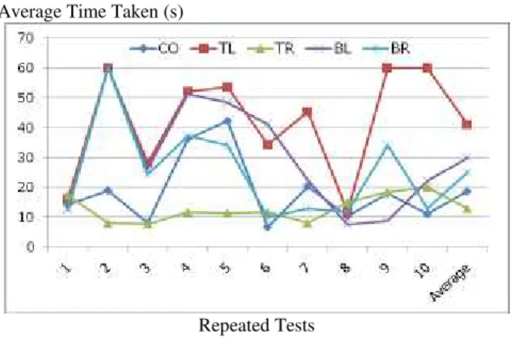
Tests were conducted for all of the evolved Pareto controllers to verify their ability in tracking the signal source robustly. The testing results showed that most of the individuals were able to achieve the target even with very few hidden units used. The robot achieved the objectives with different paths, at different time steps, and with different movements even with the same number of hidden units used. Furthermore, each of the best evolved controllers was tested for their robustness using different environmental setting as that mentioned in TL, TR, BL, BR and CO environments for 10 times, respectively. Table 6 and Fig. 12 below depict the comparison of average testing results.
TABLE6
COMPARISON OF TESTING RESULTS OBTAINED FOR DIFFERENT ROBOT’S
LOCALIZATION
Testing Environment Average Success Rate (%)
Average Time Taken (s)
TL 42.22 41.16
TR 96.67 12.79
BL 63.33 30.06
BR 71.11 25.04
CO 85.56 18.56
Average Success Rate (%)
Repeated Tests
(a) Comparison of Average Success Rate
Average Time Taken (s)
Repeated Tests
(b) Comparison of Average Time Taken
Fig 12. Testing results obtained in different robot’s localization experiment.
robust to the environment for tests performed with the TL environment. This is probably due to the fact that some of the controllers allowed the robot to turn only to the left hand side when the robot moved near to the wall. Thus, the robot might take longer distances as well as a longer amount of time to track the signal source, hence reducing its fitness scores considerably. Some cases showed the robot failed to home in towards the signal source again after moving out of the signal source area. Furthermore, in some of the outstanding cases, the evolved robots flawlessly learned to move with a straight line path to home in towards the signal source. Interestingly, one of the evolved controllers surprisingly learned wall-following to locate the signal even though this was never explicitly evaluated for in the fitness function used. Nevertheless, the robots took slightly more time to home in on the signal source because the controllers did not allow the robot to directly rotate backwards to move towards the signal. Fig. 13 depicts some of the observed robot movements from the testing phase.
(a) (b) (c)
(d) (e) (f)
(g) (h) (i)
(j) (k) (l)
(m) (n) (o)
Fig 13. Comparison of robot movements in different testing environment. (a-c) = TL, (d-f) = TR, (g-i) = BL, (j-l) = BR, and (m-o) = CO.
Three distinct robot movement behaviors were obtained during testing phases: (1) the robot learned to navigate
towards the signal source with a wall-following behavior; the robot learned to turn to its right side when it navigated near to wall, the robot also learned to navigate with maximum speed to track signal source; (2) the robot learned to navigate towards the signal source with maximum speed, the robot also successfully learned to navigate towards the signal source while keeping the straightest possible trajectory, the robot perfectly learned to avoid from bumping to the detected wall even when it was moving at the fastest speed; and (3) the robot did not learn to navigate with matching wheel speeds, thus the robot performed circular movements in tracking the signal source. Also the robot tried to stay in the signal source area as long as possible once the signal source was found, and the robot also tried to navigate back to the signal source area once it moved out from the signal source.
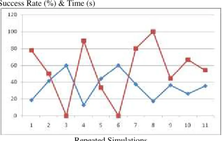
B. Inclusions of Two Obstacles
From our previous study [32], it was already reported that some initial testing results obtained using a two-obstacle environment were promising. Similarly, the generated controllers used in this experiment have never been pre-evolved for the environment similar as that used during testing phases. Furthermore, the generated controllers have been tested more extensively with 10 repeated trials in this experiment, instead of three in our previous study [32]. The testing results obtained are shown as in Fig. 14 and Table 7 below.
Success Rate (%) & Time (s)
Repeated Simulations
Fig 14. Robustness testing results obtained in two obstacles inclusions experiment.
TABLE7
COMPARISON OF TESTING RESULTS OBTAINED IN TWO OBSTACLES
INCLUSIONS EXPERIMENT
Testing Environment Average Success Rate (%)
Average Time Taken (s) Original/preserved 51.11 35.42
X + 0.05 50.56 35.34
X - 0.05 50.55 35.25
Z + 0.05 67.78 26.89
Z – 0.05 34.45 42.91
The comparison results show that the robots were robust to the environment when tests were performed in the original, Z+0.05, X+0.05 and X-0.05 environments. However, the robot was not as robust to the environment for tests performed with Z-0.05. This is probably due to the fact that some of the controllers allowed the robot to turn only to the left hand side when the robot moved near to the wall as previously observed in the prior robustness experiment. Thus, the robot might not
overcome the obstacle which had been moved further to the left. In other cases, it managed to approach but not bump into the wall and obstacles once it found the signal source. It was also observed that in some cases, the robot might not stop in the signal source area. Although it moves out of the signal source area, it still manages to turn back to the signal source area similar to a circular movement. However, some cases showed the robot failed to home in towards the signal source again after moving out of the signal source area. Furthermore, in some of the outstanding cases, the evolved robots learned to move with a straight line path to home in towards the signal source. Interestingly, the robot that learned wall-following behavior navigates with high speed to home in the signal source as well as avoid from bumping to the sensed walls and obstacles. Nevertheless, the robots took slightly more time to home in on the signal source because the controllers did not allow the robot to directly rotate backwards to move towards the signal. Fig. 15 depicts some of the observed robot movements from the testing phase.
Original
X + 0.05
X - 0.05
Z + 0.05
Z - 0.05
Fig 15. Robot movements obtained in two obstacles experiment.
Fig. 15 above clearly shows the robot was able to explore the signal source even when the controllers have never been explicitly evolved before for the testing environment used. Surprisingly, the robot was able to perform even better than our expectation compared to the previous study [32]. At the early stage of the testing phases, we found that most of the robots failed to navigate successfully to home in towards the signal source. Some robots failed to avoid from bumping to the sensed obstacles, whilst others failed to track the signal source due to the fact the obstacles used blocked most of the common paths the robot used to home in to the signal source, particularly for Z-0.05 testing results. The left hand side obstacle (Blue) has blocked one of the common paths used. Thus, those robots which learned the wall following behavior failed to home in towards the signal source. Nonetheless, for other testing environments, the robots performed quite robustly to obstacles being moved in the environment.
C. Moving RF-Signal Source
The experimental setup used in this robustness test is slightly different compared to the previous two experiments. Firstly, the signal source is no longer positioned statically at a preserved location. The signal source moves to five different locations during the testing phases. Furthermore, the duration of the robot’s evaluation lifetime is increased to 300s instead of 60s. Thus, the robot must be able to track the moving emitter and stay in the signal source area as long as possible. The testing results obtained are illustrated in Fig. 16 and Table 8 below. Each of the best evolved controllers was tested for their moving performances, tracking performances, and robustness with the different environmental setting as that mentioned in TL, TR, BR, BL, and CO for 10 times, respectively.
Average Success Rate (%)
Different RF Signal Positioning
Fig 16. Robustness testing results obtained in moving signal source experiment.
TABLE8
COMPARISON OF TESTING RESULTS OBTAINED IN MOVING SIGNAL SOURCE
EXPERIMENT
Testing Environment Average Success Rate (%)
Average Time Taken (s)
TL (0 - 60) 67.67 35.93
TR (61 - 120) 31.11 109.62
BR (121 - 180) 44.44 168.74
BL (181 - 240) 23.33 233.49
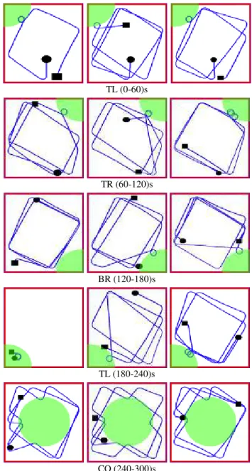
Fig. 16 clearly illustrates that most of the controllers were able to navigate towards the signal source successfully for the first 60s of the tests performed. However, the testing results showed the robot was not as robust to the environment after the signal source was moved to the TR, BR, TL, and CO locations, respectively at timesteps 60-120s, 120-180s, 180-240s, and 240-300s of the tests conducted. The tabulated testing results in Table 8 showed the robot was able to navigate towards the signal source positioned in TL with an average of 35.93s. Furthermore, the robot was able to track the signal source positioned in TR at average 109.62s, followed by tracking for the signal source localized in BR at average 168.74s. Then, the robot was able to home in towards the signal source positioned at BL corner in an average 233.49 seconds. Lastly, the robot was able to home in towards the signal source positioned at the center of the ground with an average 290.36s. This is probably due to the fact that some of the controllers allowed the robot to turn only to the left hand side when the robot moved near to the wall. In some cases, the robot managed to navigate with circular movement in the signal source area once the signal source found. Interestingly however, the robot moved to the other corners to track the signal source once the signal source moved to the different locations. Furthermore, in some of the outstanding cases, the evolved robots learned to move with a straight line path to home in towards the signal source as in the prior tests. Nevertheless, the robots took slightly more time to home in on the signal source because the controllers did not allow the robot to directly rotate backwards to move towards the signal. Some cases also showed that the robot tried to stay as long as possible in the signal source area. Interestingly, a case showed the robot was capable to stay for more than 55s out of the optimal 60s in the signal source area once the signal source detected. However, not all of the robots were able to stay longer in the signal source area. Fig. 17 depicts some of the observed robot movements from the successful testing phases.
Fig. 17 clearly shows the robots had successfully learned to navigate towards signal source even when the signal source was moved during the testing phases. Furthermore, the testing results also show that the robot was able to stay in the signal source area even if it suddenly moved out of the signal source where. In addition, the robot could also navigate back to the signal source even when it explicitly moved out of the signal source area.
IX. CONCLUSION AND FUTURE WORKS
The phototaxis behavioral testing results showed the generated controllers allowed the robot to track the light source very robustly. The RF-localization behavioral testing results showed that the generated controllers were also able to allow the robot to home in towards the RF signal source even when the robot was positioned with the back of the robot facing the emitter. Furthermore, the robustness tests also shows that the generated controllers was robust to the environment even when the controllers have never been explicitly evolved for different environments used during the testing phases. The testing results also showed that the robot was capable of exploring for the signal source even when obstacles were included in the testing environment. Hence as a conclusion, we observed that the PDE-EMO algorithm can
be practically used to robustly generate the robot controllers for phototaxis and RF-localization behaviors in autonomous mobile robots.
TL (0-60)s
TR (60-120)s
BR (120-180)s
TL (180-240)s
CO (240-300)s
Black round object = robot/starting position Rectangle object = ending location Green semi-sphere/sphere object = signal source area
Fig 17. Robot movements obtained in moving signal source experiment.
Different multifaceted environmental settings could be considered in the future experiments in order to evolve controllers that can be used in highly complex environments. The incremental evolution concept may also be considered to be used in the evolution process to start the evolution of robot controllers to perform additional new tasks with best individuals from the previous evolved task. The fitness function used plays an important role in evolving the robot controller, which is not something trivial to design. Hence, a co-evolutionary approach might also be beneficial in more complex environments where a suitably successful fitness function may be hard to identify. In addition, more experiments could be conducted by comparing the generated
controllers’ performances using different ANN architectures.
ACKNOWLEDGMENT
This research work is funded under the ScienceFund project SCF0002-ICT-2006 granted by the Ministry of Science, Technology and Innovation, Malaysia.
REFERENCES
[1] Floreano, D., and Urzelai, J. ―Evolutionary Robots: The Next Generation,‖ In Proceedings of the Seventh International Symposium on Evolutionary Robotics (ER2000), From Intelligent Robots to Artificial Life. AAI Books, 2000, 231–266.
[2] Nelson, A.L., and Grant, E. Developmental analysis in Evolutionary Robotics. Adaptive and Learning Systems, IEEE Mountain Workshop on IEEE CNF, 2006, 201-206.
[3] Pratihar, D.K. Evolutionary robotics – A Review. Sadhan., 28, 6 (Dec. 2003), 999-1009.
[4] Teo, J. Evolutionary Multi-Objective Optimization for Automatic Synthesis of Artificial Neural Network Robot Controllers. Malaysian Journal of Computer Science, volume 18, number 2, 2005, pp 54-62. [5] Teo, J. ―Darwin + Robots = Evolutionary Robotics: Challenges in
Automatic Robot Synthesis‖. 2nd International Conference on Artificial Intelligence in Engineering and Technology (ICAET 2004).
Kota Kinabablu, Sabah, Malaysia, August 2004, Vol 1, pp 7-13. [6] Floreano, D., and Mondada, F. Evolution of homing navigation in a
real mobile robot. IEEE Transactions on Systems, Man, and Cybernetics-Part B, 26:396—407, 1996.
[7] Alba, E., and Tomassini, M. Parallelism and Evolutionary Algorithms.
IEEE Transactions on Evolutionary Computation. IEEE Press, 6(5):443-462, October 2002.
[8] Urzelai, J., and Floreano D., Evolutionary Robots with Fast Adaptive Behavior in New Environments. Third International Conference on Evolvable Systems: From Biology to Hardware (ICES2000),
Edinburgh, Scotland (UK), 17-19 April 2000.
[9] Carlos, A. Coello Coello. Recent Trends in Evolutionary Multiobjective Optimization, in Ajith Abraham, Lakhmi Jain and Robert Goldberg (editors), Evolutionary Multiobjective Optimization: Theoretical Advances And Applications, pp. 7--32, Springer-Verlag, London, ISBN 1-85233-787-7, 2005.
[10] Floreano, D., and Urzelai, J. Evolutionary On-Line Self-Organization of Autonomous Robots. In Sugisaka, M. (ed.) Proceedings of the 5th International Symposium on Artificial Life and Robotics (AROB'2000), Oita (JP), January 2000.
[11] Horchler, A., Reeve, R., Webb, B. and Quinn, R. Robot phonotaxis in the wild: a biologically inspired approach to outdoor sound localization. Advanced Robotics (2004), 18(8):801-816
[12] Reeve, R., Webb, B., Horchler, A., Indiveri, G., and Quinn, R. New Technologies for testing a model of cricket phonotaxis on an outdoor robot platform. Robotics and Autonomous Systems, 2005, 51(1):41-54.
[13] Blow, M. Evolutionary Robotics Simulation using a CTRNN. MSc., Artificial Life Project report, 2003.
[14] Meeden L.A. An Incremental Approach to Developing Intelligent Neural Network Controllers for Robots. IEEE Trans. Sys., Man, and Cybern., 26(3), June 1996, 474-485.
[15] Nehmzow, U. Physically Embedded Genetic Algorithm Learning in Multi-Robot Scenarios: The PEGA algorithm.
[16] Pugh, J., and Martinoli, A. Multi-robot Learning with Particle Swarm Optimization. In Proceedings of the fifth international joint conference on Autonomous agents and multiagent systems (Hakodate, Japan, 2006). ACM Press, New York, USA, 2006, 441-448. [17] Teo, J. Pareto Multiobjective Evolution of Legged Embodied
Organisms. Ph.D. Thesis, University of New South Wales, New South Wales, 2003.
[18] Elaoud, S., Loukil, T., and Teghem, J. The Pareto Fitness Genetic Algorithm: Test Function Study. European Jurnal of Operational Research, 177 (2007), 1703-1719.
[19] Gibson, R. (2007, Oct 30). Radio and television reporting. Boston: Allyn and Bacon. [Online]. Available:
http://www.fdv.uni-lj.si/Predmeti/Dodiplomski/Arhiv/ucni_nacrti_20 02-03.pdf
[20] Pike, J. (2007, Oct 30). GPS Overview from the NAVSTAR Joint Program Office. [Online]. Available:
http://www.fas.org/spp/military/program/nav/gps.htm
[21] NOAA Satellite and Information Service, (2008, May 03), Search, Rescue and Tracking. [Online]. Available:
http://www.sarsat.noaa.gov/
[22] Zitzler, E., Laummann, M., and Bleuler, S. A Tutorial on Evolutionary Multiobjective Optimization. Proceedings of the Workshop on Multiple Objective Metaheuristics. Springer-Verlag, 2004.
[23] Zitzler, E., Laumanns, M., and Bleuler, S. A. Tutorial on Evolutionary Multiobjective Optimization, Lecture Notes in Economics and Mathematical Systems. Springer, 535, 2004, 3-37.
[24] Zitzler, E., Deb, K., and Thiele, L. (in press) Comparison of multiobjective evolutionary algorithms: Empirical results. Evolutionary Computation, 8.
[25] Abbass, H.A., Sarker, R., and Newton, C. PDE: A Pareto-frontier Differential Evolution Approach for Multi-objective Optimization Problems, Proceedings of the Congress on Evolutionary Computation 2001 (CEC'2001), Vol. 2, IEEE Service Center, Piscataway, New Jersey, pp. 971--978, May 2001.
[26] Karaboğa, D., and Őkdem, S. A Simple and Global Optimization Algorithm for Engineering Problems: Differential Evolution Algorithm. Turk J Elec Engin. Vol.12, No.1. 2004, TŰBİTAK. [27] Storn, R., and Price, K. “Differential evolution: A simple and efficient
adaptive scheme for global optimization over continuous spaces”.
Technical Report TR-95-012, 1995, International Computer Science Institute, Berkeley.
[28] Deb, K. Multi-Objective Optimization using Evolutionary Algorithms. Addison-Wesley, WS, 2001.
[29] Kukkonen, S. Ranking-Dominance and Many-Objective Optimization. IEEE Congress on Evolutionary Computation (CEC 2007). Singapore. 2007, pp 3983-3990.
[30] Michel, O. Cyberbotics Ltd Webots: Professional Mobile Robot Simulation, International Journal of Advanced Robotics Systems, 1, 1(2004), 39-42.
[31] K. O. Chin, Teo. J, and S. Azali, "Multi-objective Artificial Evolution of RF-Localization behavior and Neural Structures in Mobile Robots,"
IEEE World Congress on Computational Intelligence (WCCI-CEC'08), Hong Kong. 1-6 June 2008.
[32] K. O. Chin, Teo. J, and S. Azali, "Multi-objective Controller Evolution of RF Localization for Mobile Autonomous Robots," 2008 IEEE Conference on Soft Computing in Industrial Application (SMCIA'08),
Muroran Hokkaido, Japan. 25-27 June 2008.
Chin Kim On was born in Tawau, Sabah, Malaysia,
in 1979. The author received his Master Degree in Software Engineering with the University of Malaysia Sabah, Sabah, Malaysia in 2005. The author’s research interests included the evolutionary multi-objective optimization, evolutionary computing, evolutionary robotics, neural networks, image processing, and biometric security system with main focus on fingerprint and voice recognition.
He is currently pursuing his PhD in the research area of evolutionary robotics using multi-objective optimization for RF-localization and swarm behavior under the Universiti Malaysia Sabah in the School of Engineering and Information Technology, Sabah, Malaysia. He acted as a Lecturer for 6 months in the information technology department at the Kolej of Tunku Abdul Rahman, Sabah Branch, before he continued his PhD study. Currently, he has over 15 book chapters, journals, and peer-reviewed paper publications in the areas of biometric security system, fingerprint recognition, voice recognition, image processing, evolutionary robotics and evolutionary computing.
Mr. Kim On is a student member of IEEE and IAENG societies.
Jason Teo was born in Sibu, Sarawak, Malaysia, in
1973. The author received his Doctoral in Information Technology degree from the University of New South Wales at the Australia Defense Force Academy in 2003, researching Pareto artificial evolution of virtual legged organisms. The author’s research interests included focus on the theory and applications of evolutionary multi-objective optimization algorithms in co-evolution, robotics and metaheuristics.
of the School of Engineering and Information Technology, Universiti Malaysia Sabah. Currently, he has over 100 publications including book chapters, journals, and peer-reviewed conference publications in the areas of artificial life, evolutionary robotics, evolutionary computing and swarm intelligence.
Dr. Jason is a professional member of the ACM and IEEE societies since year 2005 and 2006 respectively and has been the grantee of a number of research grants under the Ministry of Higher Education and Ministry of Science, Technology and Innovation, Malaysia.