www.ann-geophys.net/29/1827/2011/ doi:10.5194/angeo-29-1827-2011
© Author(s) 2011. CC Attribution 3.0 License.
Annales
Geophysicae
Coordinated Cluster/Double Star and ground-based observations of
dayside reconnection signatures on 11 February 2004
Q.-H. Zhang1, M. W. Dunlop2, R.-Y. Liu1, H.-G. Yang1, H.-Q. Hu1, B.-C. Zhang1, M. Lester3, Y. V. Bogdanova4, I. W. McCrea2, Z.-J. Hu1, S. R. Crothers2, C. La Hoz5, and C. P. Nielsen6
1SOA Key Laboratory for Polar Science, Polar Research Institute of China, Shanghai, China 2Space Science Department, Rutherford-Appleton Laboratory, Chilton, Didcot, UK
3Department of physics and Astronomy, University of Leicester, Leicester, UK 4Mullard Space Science Laboratory, University College London, Dorking, Surrey, UK 5Department of Physics, Faculty of Science, University of Tromsø, 9037 Tromsø, Norway 6Norwegian Polar Institute, Sverdrupstasjonen, 9173 Ny-Alesund, Norway
Received: 27 November 2010 – Revised: 29 August 2011 – Accepted: 13 October 2011 – Published: 24 October 2011
Abstract. A number of flux transfer events (FTEs) were
ob-served between 09:00 and 12:00 UT on 11 February 2004, during southward and dawnward IMF, while the Cluster spacecraft array moved outbound through the northern, high-altitude cusp and dayside high-latitude boundary layer, and the Double Star TC-1 spacecraft was crossing the dayside low-latitude magnetopause into the magnetosheath south of the ecliptic plane. The Cluster array grazed the equato-rial cusp boundary, observing reconnection-like mixing of magnetosheath and magnetospheric plasma populations. In an adjacent interval, TC-1 sampled a series of sometimes none standard FTEs, but also with mixed magnetosheath and magnetospheric plasma populations, near the magne-topause crossing and later showed additional (possibly tur-bulent) activity not characteristic of FTEs when it was sit-uated deeper in the magnetosheath. The motion of these FTEs are analyzed in some detail to compare to simultane-ous, poleward-moving plasma concentration enhancements recorded by EISCAT Svalbard Radar (ESR) and “poleward-moving radar auroral forms” (PMRAFs) on the CUTLASS Finland and Kerguelen Super Dual Auroral Radar Network (SuperDARN) radar measurements. Conjugate SuperDARN observations show a predominantly two-cell convection pat-tern in the Northern and Southern Hemispheres. The results are consistent with the expected motion of reconnected mag-netic flux tubes, arising from a predominantly sub-solar re-connection site. Here, we are able to track north and south in closely adjacent intervals as well as to map to the corre-sponding ionospheric footprints of the implied flux tubes and demonstrate these are temporally correlated with clear
iono-Correspondence to: Q.-H. Zhang ([email protected])
spheric velocity enhancements, having northward (south-ward) and eastward (west(south-ward) convected flow components in the Northern (Southern) Hemisphere. The durations of these enhancements might imply that the evolution time of the FTEs is about 18–22 min from their origin on topause (at reconnection site) to their addition to the magne-totail lobe. However, the ionospheric response time in the Northern Hemisphere is about 2–4 min longer than the re-sponse time in the Southern Hemisphere.
Keywords. Magnetospheric physics (Magnetopause, cusp,
and boundary layers; Magnetosphere-ionosphere interac-tions) – Space plasma physics (Magnetic reconnection)
1 Introduction
Paschmann et al., 1982) and their larger occurrence rate dur-ing periods of southward interplanetary magnetic field (IMF) (e.g. Berchem and Russell, 1984; Lockwood and Smith, 1992). Statistical studies (e.g. Rijnbeek et al., 1984; Lock-wood, 1991; Lockwood and Wild, 1993) have also shown that the mean interval between FTE signatures is of the order of 8 min. However, Lockwood and Wild (1993) showed that the distribution of these intervals has a mode value at 3 min, with upper and lower decile values of 1.5 and 18.5 min, re-spectively.
Because of the limitation of single-point spacecraft mea-surements at the magnetopause, it is difficult to determine the spatial distribution and motion of FTEs. Furthermore, the in-situ space observations are associated with the re-sponse of the ionosphere and ground geomagnetic field. The early work of Elphic et al. (1990) demonstrated that ionospheric flow bursts measured by EISCAT were associ-ated with FTEs observed by ISEE and the first magneti-cally conjugate measurements of an FTE by Equator-S and of ionospheric flow bursts by SuperDARN were presented by Neudegg et al. (1999). The UV aurora measured by the Polar spacecraft’s VIS (Visible Imaging System) Earth cam-era in the vicinity of the reconnection footprint for this event was later discussed (Neudegg et al., 2001). Recently, Cluster (Escoubet et al., 2001) observations of FTEs (e.g. Owen et al., 2001; Fear et al., 2005; Zheng et al., 2005; Hasegawa et al., 2006; Wang et al., 2005) have been combined with a vari-ety of ground-based instruments (e.g. Lockwood et al., 2001; Wild et al., 2001, 2003; Marchaudon et al., 2004; Zhang et al., 2008, 2010).
Following the successful launch of Double Star, it is now possible to study FTEs from five or six points in space si-multaneously. For example, the first magnetically conjugate observations of FTEs by Cluster and Double Star TC-1 at the Northern and Southern Hemisphere, respectively, were presented by Dunlop et al. (2005) and coordinated Clus-ter/Double Star and ground-based measurements of FTEs were reported by Wild et al. (2005, 2007). Nevertheless, the evolution of a flux tube (FTE), from its generation at the mag-netopause to its disappearance in the global magnetospheric convection (Amm et al., 2005) is not well tied to the location of reconnection onset or the development of the reconnection rates.
In this paper, we analyze several medium to large scale FTEs which were observed by the Cluster array, at the high-latitude magnetopause, or by the TC-1 spacecraft, south of the subsolar magnetopause, simultaneously measured by the ESR and conjugately observed by the CUTLASS Finland and Kerguelen SuperDARN radars (also observing the iono-spheric plasma flow, Greenwald et al., 1995; Chisham et al., 2007) measuring the global ionospheric convection. These FTEs are interpreted as reconnection generated signatures. All FTEs observed by Cluster and TC-1 have some recon-nection features in the plasma data: some of these FTEs, especially observed by TC-1, contain an accelerated
mag-netosheath population, and the others contain a mixture of magnetospheric and magnetosheath plasma populations. Us-ing the Cluster 4-spacecraft observations, we calculate the velocity and the size of the implied flux tubes connected to the northern cusp. The ESR measurements, record pole-ward flows and the CUTLASS Finland and Kerguelen Su-perDARN radar observations show “poleward-moving radar auroral forms” (PMRAFs), also indicative of bursty recon-nection at the dayside magnetopause. The SuperDARN ob-servations show that the individual flux tube movements, which contain predominantly northward (southward) or east-ward (westeast-ward) components, map to positions in the iono-spheric convection cells in the Northern (Southern) Hemi-sphere which have the corresponding flow directions. More-over, we verify that the movements of the reconnected flux tubes are well consistent with the Cooling model (Cooling et al., 2001), which predicts the expected motion of recon-nected flux tubes, given the prevailing IMF and sheared solar wind flow. We also comment on other features of the data, focusing on additional magnetic activity at TC-1.
2 Observations
2.1 Upstream solar wind and IMF conditions
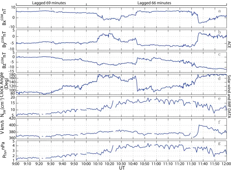
Figure 1 presents an overview of the solar wind and IMF conditions measured by the ACE satellite. Parameters shown are IMF components (a)BX, (b)BY, (c)BZ, (d) IMF clock
angle, (e) solar wind plasma number density, (f) solar wind speed, and (g) solar wind dynamic pressure. The data have been lagged by 69 min before 10:00 UT (lagged time) and 66 min after 10:00 UT (this time delay is calculated using the method of Liou et al., 1998) in order to take into account the propagation of solar wind/IMF structure from the space-craft to the subsolar magnetopause. The ACE spacespace-craft is located at about (221.2,−32.6, 9.5)REin the Geocentric
So-lar Magnetic (GSM) coordinate system at about 10:34 UT (lagged time). During whole interval, the IMF BZ
com-ponent was near zero before about 09:30 UT (lagged time) and always negative, varying between−8.2 to−0.4 nT (see Fig. 1c), after 09:30 UT, while theBYcomponent was
nega-tive with a short, posinega-tive incursion (see Fig. 1b). The IMF clock angle (if BZ>0, clock angle = atan(|BY|/BZ), and if BZ<0, the clock angle =π−atan(|BY|/BZ)) therefore
var-ied between 90◦ and 180◦during this period (see Fig. 1d).
The solar wind density increased from 7 to 19 cm−3over the
interval of interest (see Fig. 1e), whilst the solar wind veloc-ity varied between 370 and 387 km s−1(see Fig. 1f), resulting in a prevailing solar wind dynamic pressure of∼1.8–4.5 nPa (see Fig. 1g).
2.2 Spacecraft and ground coverage
9:00 9:10 9:20 9:30 9:40 9:50 10:00 10:10 10:20 10:30 10:40 10:50 11:00 11:10 11:20 11:30 11:40 11:50 12:001 2
3 4 5
P
Dyn
nPa
UT
360380 400 420
V km/
s
5 10 15 20
N (cm )
SW80 100 120 140 160 180
Clock Angle
-15 -10 -5 0 5
Bz
GSM
nT
-10 -5 0 5
By
GSM
nT
-10 0 10
Bx
GSM
nT
ACE Solar wind and IMF DATA
Lagged 69 minutes Lagged 66 minutes
(Deg)
D
E
F
G
H
I
J
Fig. 1. An overview of the solar wind and IMF conditions measured by the ACE satellite. Parameters shown are IMF components (a)BX,
(b)BY, (c)BZ, (d) IMF clock angle, (e) solar wind plasma number density, (f) solar wind speed, and (g) solar wind dynamic pressure.
with a perigee at∼4RE, an apogee at∼19.6REand
identi-cal orbital periods of 57 h. The average distance of each two spacecraft is about 300 km in February 2004. Data with 4 s resolution from the fluxgate magnetometer (FGM) (Balogh et al., 2001) on all four Cluster satellites and from the Plasma Electron and Current Experiment (PEACE) (Johnstone et al., 1997) and from Cluster Ion Spectrometry (CIS) (R`eme et al., 2001) onboard Cluster S/C 1 are used in this study. One of the two Double Star spacecraft, TC-1 (Liu et al., 2005) was launched in December 2003 into an equatorial orbit at 28.2◦ inclination, with a perigee altitude of 577 km, an apogee of 13.4RE, and an orbital period of 27.4 h. Data with 4 s
resolu-tion from FGM (Carr et al., 2005) and from PEACE (Fazak-erley et al., 2005) instruments onboard TC-1 are used in this paper.
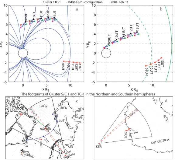
Figure 2 shows the tracks of all Cluster and the TC-1 spacecraft between 09:00 and TC-13:00 UT on TC-1TC-1 Febru-ary 2004, in the X-Z (a) and X-Y (b) planes, in the GSM co-ordinate system, with the configuration of the Cluster
space-craft array drawn as a tetrahedron (size scaled up by a fac-tor of 20). Model geomagnetic field lines are shown for the projection into the X-Z plane and cuts through the bow shock (BS) and magnetopause (MP) are shown for the X-Y plane. The ionospheric footprints of Cluster spacecraft 1 (in blue line) and TC-1 (in red line) spacecraft on the maps of Northern (c) and Southern (d) Hemispheres in geographic coordinate system are shown in the lower panels. The X-Z plane field lines and ionospheric footprints of the spacecraft are drawn from the Tsyganenko ’96 model (Tsyganenko and Stern, 1996) with input parameters: PDyn=3.93 nPa (the
solar wind dynamic pressure), IMF BY= −4.00 nT, IMF BZ= −5.92 nT and Dst =−1 nT. These parameters
0 5 10 -6
-4 -2 0 2 4 6 8 10
X R
Z R
Cluster / TC-1 - Orbit & s/c - configuration 2004 Feb 11
10UT
11UT
10UT 12UT 13UT
09UT
11UT 12UT 13UT
09UT
E
E
0 5 10
-6 -4 -2 0 2 4 6 8 10
Y R
X R
10U
T
10U
T
13UT
12U
T
11U
T
09U
T
09U
T 11U
T
12U
T
13U
T
E
E
D E
GREENLAND
ICELAND
The footprints of Cluster S/C 1 and TC-1 in the Northern and Southern hemispheres
90° N 80
70° N
° N
FINLAND 09UT
10UT
11UT
12UT
13UT 09UT
HAN
NAL
beam 8
ANTARCTICA
10UT
90 ° S
75
°
S
09UT
KER
F G
beam 12
Fig. 2. All Cluster and TC-1 spacecraft tracks in the X-Z (a) and X-Y (b) plane in GSM coordinates, together with the ionospheric footprints
of Cluster S/C 1 (blue line) and TC-1 spacecraft (red line) on the maps of Northern (c) and Southern (d) Hemispheres, between 09:00 and 13:00 UT on 11 February 2004. The orbit also shows the configuration of the Cluster spacecraft array as a tetrahedron (size scaled up by a factor of 20). The Model geomagnetic field lines are shown for the projection into the X-Z plane and cuts through the bow shock and magnetopause are shown for the X-Y plane. The X-Z plane field lines and ionospheric footprints of the spacecraft are drawn from the Tsyganenko ’96 model inputting the real parameters. The field-of-view of the CUTLASS Finland radar and Kerguelen radar is presented as a fan in panels(c) and (d), respectively, with the beams employed in this study indicated by red dashed lines. The poleward-looking low elevation beam (32M dish) of ESR (between 76 and 85◦magnetic latitude) is indicated by the solid green line. The red“⊕” presents the magnetic pole.
about 10:00 UT. Thus there are no Cluster footprints in the Southern Hemisphere and TC-1 footprints end after about 10:00 UT in both hemispheres. In fact, the data shown be-low (see Fig. 3) indicate that Cluster exits into the magne-tosheath earlier at∼11:20 UT and TC-1 exits at∼09:20 UT, which suggests a significantly eroded magnetopause at this time. The field-of-view of the CUTLASS Finland and Ker-guelen SuperDARN radar is presented as a fan in Fig. 2c and d, respectively, with the beam employed in this study indi-cated by red dashed lines. The poleward-looking low eleva-tion beam (32M dish) of ESR (between 76 and 85◦magnetic
latitude) is indicated by the solid green line in Fig. 2c. The red “⊕” represents the magnetic pole.
2.3 Cluster and Double Star TC-1 observations
0 100 200
|B| nT
−80 −60 −40 −20 0 20 40
B N
nT
−100 −50 0 50
B M
nT
−150 −100 −50 0 50 100
B L
nT
100 80 120 140 160 180
Clock angle Deg
(lagged 69/66min)
C1 LEEA and HEEA Parallel
10 -6
10 -5
10 -4 10 -3
ergs
/cm
**
2-s-str-eV
dEF
TC1 HEEA Parallel
10 -6
10 -5
10 -4
10 -3
ergs
/cm
**
2-s-str-eV
dEF
10 2
10 3
10 4
C
enter Energy
eV
10 1
10 1
10 2
10 3
10 4
09:00 09:30 10:00 10:30 11:00 11:30 12:00
Center Energy
eV
UT
9:00 9:30 10:00 10:30 11:00 11:30 12:00
Cluster/Double Star (TC-1) FGM (minimum variance) 2004 Feb 11
)7( i MP ii 1 MP 2
H
I
J D
E
F
G
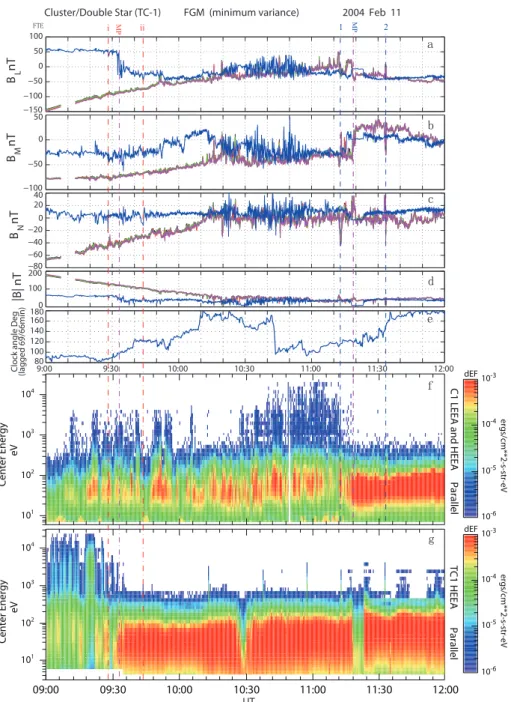
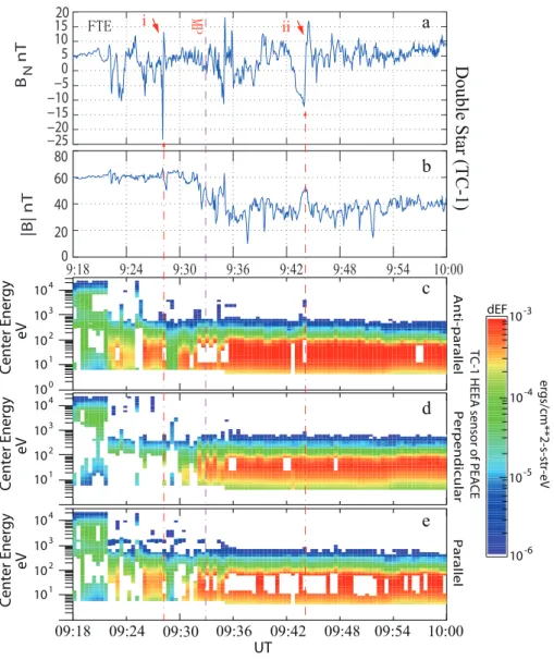
Fig. 3. An overview of the FGM measurements which are projected onto a LMN coordinates, and the lagged IMF clock angle, together with
the spectrograms of electron field-aligned differential energy flux from the HEEA and LEEA sensor of PEACE on the Cluster S/C 1 and from PEACE instrument on TC-1, between 09:00 and 12:00 UT on 11 February 2004. Here highlight two FTEs observed by TC-1 by red dashed vertical lines, and two FTEs measured by Cluster by blue dashed vertical lines, respectively. There also marked the magnetopause crossing at about 09:33 UT for TC-1 and about 11:18 UT for Cluster by violet dashed vertical lines.
11:13, and 11:33 UT) are believed to be spacecraft gener-ated interference spikes. The dropouts in the TC-1 distribu-tion around 10:30 and 11:20 UT are excursions into the so-lar wind (encountering the bow shock), which is also clear from the TC-1 magnetic field (see Fig. 3), and it is clear that the second of these corresponds to the main magnetopause crossing by Cluster, suggesting a global compression of the magnetosphere and inward bow shock motion at this time.
−15 −10 −5 0 5 10 15 20 −50
−45 −40 −35 −30 −25 −20 −15
S
BL
(nT)
BN (nT)
−40 −35 −30 −25 −20 −15 −50
−45 −40 −35 −30 −25 −20 −15
S
BL
(nT)
BM (nT)
DSP TC−1 1 Hodogram of Magnetic field 2004 Feb 11 09:43:0.892−09:45:25.842
−50 −40 −30 −20 −10 0 10 20 30 −30
−20 −10 0 10 20 30 40 50
S
BL
(nT)
BN (nT)
5 10 15 20 25 30 35 40 45 −30
−20 −10 0 10 20 30 40 50
S
BL
(nT)
BM (nT)
Cluster 1 Hodogram of Magnetic field 2004 Feb 11 11:32:42.938−11:33:39.473
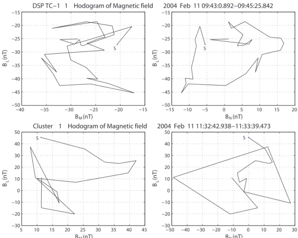
Fig. 4. Hodograms of the magnetic field in LMN coordinates for the periods 09:43:01–09:45:26 UT observed by TC-1 spacecraft and for
the periods 11:32:43–11:33:39 UT measured by Cluster 1. Left and right panels show L-M and L-N representations. The black dot point (marked by “S”) presents the start point in each panel.
the boundary normal. The unit vectorsl,m,nare given as (−0.40, 0.40, 0.83), (0.56, 0.82, −0.12) and (0.72, −0.42, 0.55) in GSM coordinates, for the mean Cluster magne-topause crossing, and (0.38, 0.32, 0.87), (0.09, 0.92,−0.38) and (0.92,−0.22,−0.31) in GSM coordinates, for TC-1. In-spection of the solar wind conditions shows that the IMF clock angle (see Fig. 3e) exhibited stable, dominant south-ward IMF conditions (CA ∼130◦ to 180◦) between about 09:54 and 10:43 UT and after 11:30 UT, and variable dom-inant dawnward IMF conditions (CA ∼80◦ to 140◦) with southward components before 09:54 UT and between 10:43 and 11:30 UT. This favours a high reconnection rate at the low-latitude magnetopause. Figure 3a and f shows disturbed magnetic field and precipating electron signatures, which in-dicates that the Cluster spacecraft were crossing open field line regions and cusp between about 09:10 and 11:12 UT and encountered the magnetopause at about 11:18 UT (marked by violet dashed vertical line in Fig. 3). The spacecraft were in the magnetosheath after about 11:18 UT. Figure 3g shows the TC-1 spacecraft was moving outbound through the dayside, low-latitude magnetopause at about 09:33 UT and within the magnetosheath after that with two short
ex-cursions into the solar wind. There are a large number of separate field parallel electron beams containing mixed high-and low-energy electron populations in the Cluster S/C 1 electron spectrogram (Fig. 3f). There are a large number of electron beams in the TC-1 PEACE electron spectrograms (Fig. 3g), although these beams consists mostly of accel-erated magnetosheath population. The small-scale electron signatures observed in the magnetosheath by TC-1 are quite complicated: some electron beams are very short and have high electron fluxes at 90 deg pitch-angles. Some beams are longer and show reconnection-related signatures. These will be discussed later in the text in detail.
10 1
10 2
10 3
10 4
Center Energy
eV
10 1
10 2
10 3
10 4
Center Energy
eV
10 1
10 0
10 2
10 3
10 4
Center Energy
eV
09:30 10:00
TC-1 HEEA sensor of PEACE
10 -6
10 -5
10 -4
10 -3
ergs/cm**2-s-str-eV
dEF
UT
09:18 09:24 09:36 09:42 09:48 09:54
9:18 9:24 9:30 9:36 9:42 9:48 9:54 10:00
0 20 40 60 80
|B| nT
−25 −20 −15
−10 −5
0 5 10
15 20
B N
nT
)7( i 03
Double Star (TC-1)
a
b
e
c
d
iiAnti-parallel
Perpendicular
Parallel
Fig. 5. Zoom in of the magnetic field boundary normal componentBN(same as Fig. 3c) and the field magnitude, together with PEACE
electron spectrograms in anti-parallel, perpendicular, and parallel directions, observed by TC-1.
by Cluster and TC-1, respectively. As an example, Fig. 4 presents hodograms of the magnetic field in LMN coordi-nates for the periods 09:43:01–09:45:26 UT observed by TC-1 spacecraft and for the periods TC-1TC-1:32:43–TC-1TC-1:33:39 UT mea-sured by Cluster S/C 1. Left and right panels show L-M and L-N representations. The black dot point (marked by “S”) presents the start point in each panel. From Fig. 4, we find that there were clear “bump” of the reconnected flux tube in both L-M and L-N planes of the magnetic field crossed by TC-1 and Cluster, respectively, which indicated that the FTE-like signatures are FTEs and could be thought as one of the criteria of the FTE identifications. According to the crite-rion from the hodogram analysis with higher plasma number density and velocity, we highlight for detailed analysis, one magnetospheric and one magnetosheath FTEs measured by TC-1 (indicated by red dashed vertical lines and marked by
the red numbers “i–ii” at the top of Figs. 3 and 5), and two other FTEs observed by Cluster (indicated by blue dashed vertical lines and marked by the blue numbers “1–2” at the top of Figs. 3 and 6), respectively. These data are plotted in Figs. 5 and 6 for interval of 09:18–10:00 UT for TC-1 and 11:00–12:00 UT for Cluster S/C 1 respectively to show more detail for the analysis below.
The panels in Fig. 5 show the magnetic field boundary normal componentBN(same as Fig. 3c) and the field
10-6 10-5 10-4ergs/cm**2-s-str-eV dE F
Anti-parallel
CL-1 LEEA and HEEA Zone
Perpendicular
Parallel
e
f
g
−300 −200 −100 0 100 200 3000 5 10 15 20 25 300 50 100 −60 −40 −20 0 20 40
101 102 103 104
Center Energy
eV
101 102 103 104
101 102 103 104
Center Energy
eV
101 102 103 104
100 101 102 103 104
Center Energy
eV
100 101 102 103 104
11:00 11:10 11:20 11:30 11:40 11:50 12:00
UT
11:00 11:05 11:10 11:15 11:20 11:25 11:30 11:35 11:40 11:45 11:50 11:55 12:00
V
km/s
N
H
cm
-3
+
H
+
VN VM VL
|B| nT
B
N
nT Cluster S/C 1
2 1
FTE a
b
c
d
MP
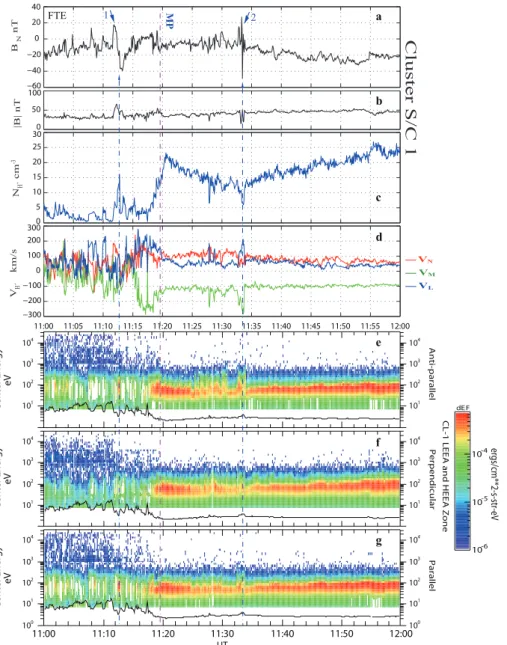
Fig. 6. Zoom in of (a) the magnetic field boundary normal componentBN (same as Fig. 3c), (b) the field magnitude, (c) the number
density and (d) velocity (projected into LMN coordinates) of H+from CIS instrument onboard Cluster S/C 1, together with PEACE electron spectrograms in the (e) anti-parallel, (f) perpendicular, and (g) parallel directions, observed by Cluster S/C 1.
bipolar signatures in theBN component (highlighted by the
red dashed vertical lines and marked by the red numbers “i– ii”). This suggests that TC-1 observed southward moving flux tubes, which are connected to the southern cusp and were generated by low-latitude magnetic reconnection. The electron population was studied in detail for these two FTEs, using electron spectrogram and electron pitch-angle spectro-gram (not shown here). The electron spectrospectro-gram shows the well-defined electron beam with accelerated magnetosheath plasma population mixed with the magnetospheric popula-tion for the second discussed FTE (ii). However there is no clear electron signature associated with the first FTE (i),
pitch-angle spectrogram (not shown here) for this period. We note that these observations are very similar to the observa-tions presented by Retino et al. (2007) of the reconnection inside the turbulent magnetosheath. We suggest, as the TC-1 spacecraft lies deeper in the magnetosheath during this inter-val, that the observed magnetic field fluctuations and electron small scale sub-structure are not associated with FTEs, but with more complex processes which are out of scope of this paper.
In Fig. 6 we present (a) the magnetic field boundary nor-mal componentBN (same as Fig. 3c), (b) the field
magni-tude, (c) the number density and (d) velocity (projected into LMN coordinates) of H+from CIS instrument onboard Clus-ter S/C 1, together with (e) the PEACE electron spectrograms in the (e) anti-parallel, (f) perpendicular, and (g) parallel di-rections, as observed by Cluster S/C 1 in the same way as Fig. 5. There are associated FTE signatures in the Cluster magnetic field data. As in Fig. 3, we indicate the two FTEs, observed by Cluster, by blue dashed vertical lines. All FTEs show standard polarity (positive/negative) bipolar signatures in theBN component (see Fig. 6a) with enhanced|B|,
en-hanced number density of H+ (decreased number density of H+ in magnetosheath FTE) with fast ion flow in L and M direction (see Fig. 6c and d), and well defined electron beams, in which the plasma mainly focused on the paral-lel or anti-paralparal-lel directions, with a clear mixing of magne-tosheath and magnetospheric plasma populations in the elec-tron spectrograms for the first FTE and accelerated magne-tosheath population for the second FTE (see Fig. 6e–i). This suggests that Cluster observed northward moving flux tubes, which are connected to the northern cusp and were gener-ated by low-latitude magnetic reconnection. These FTE sig-natures become increasingly distinct and of larger size as the spacecraft cross the magnetopause into the magnetosheath. Additionally, for the earlier period shown in Fig. 3, be-tween 09:00–10:00 UT, while Cluster was grazing the pole-ward cusp boundary, there appear to be a large number of often non-standard (positive/negative) FTE-like signatures. These therefore might represent a range of flux tube sizes (as discussed in Sect. 3). The electron spectrograms of Clus-ter S/C 1 also show clear mixing of magnetosheath and mag-netospheric plasma population signatures suggestive of the reconnection features expected for each FTE.
2.4 EISCAT measurements
We now briefly examine the ionospheric dynamics which re-sulted from the FTEs discussed above.
Data from the two-dish incoherent scatter radar system near Longyearbyen, part of the EISCAT Svalbard Radars (ESR) (Wannberg et al., 1997) are used here. One dish (a 32m parabolic antenna) is fully steerable towards any direc-tion, and the other (a 42 m parabolic antenna) is fixed, point-ing along the local magnetic field line. On the 11 Febru-ary 2004, the 32 m-dish was pointing nearly towards
geo-magnetic north (azimuth 336◦), at low elevation (30◦). The
radars used alternating code measurement techniques to pro-vide profiles of electron density, electron and ion tempera-ture, and ion velocity along the line-of-sight.
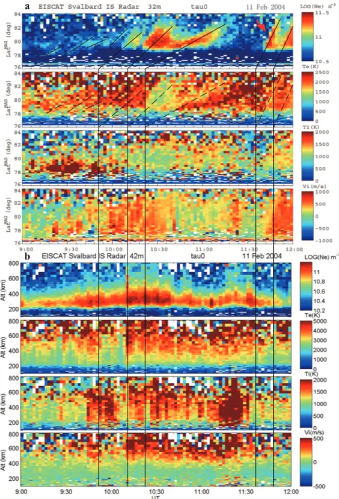
During the interval of interest, the ionosphere above Sval-bard was magnetically conjugate to Cluster and the radar measurements suggest that it was subject to impulsive pre-cipitation associated with FTE-related bursts of magne-topause reconnection. Figure 7, for example, presents 2-min post-integrations of the ESR radar observations between 09:00 and 12:00 UT (the same interval as in Fig. 3). Fig-ure 7a presents observations of the electron density, the elec-tron temperature, the ion temperature, and the line-of-sight ion velocity from the low elevation northward-directed ESR dish (azimuth 336◦, elevation 30◦). The post-integrated data are shown as a function of magnetic latitude between 76◦and
84◦ and the observations cover the F-region altitude range
from about 100 to 520 km. The density measurements indi-cated a series of high-density plasma regions moving along the beam to higher latitudes (highlighted by the black solid lines in the first panel of Fig. 7a), so called poleward-moving plasma concentration enhancements, some of which could correspond, one-to-one to the FTEs observed by TC-1 or Cluster. For example, the one highlighted by red arrow could correspond to the FTE 2 observed by Cluster. These events appeared quasi-periodically with a period of about 10 min, which is roughly consistent with the period of FTEs observed by Cluster and TC-1 spacecraft. It is worth not-ing that the density measurements indicated a density of 3×10¹¹m−3between 79◦and 82◦geomagnetic latitude (see the first panel of Fig. 7a) in the events between about 10:10 and 11:10 UT and after about 11:42 UT. The electron tem-perature decreased in these events, highlighted by the black dashed bias lines (see the second panel of Fig. 7a). These suggest that the transient reconnection (FTE) leads to the ero-sion of the OCB equatorward to a region of higher density plasma (the solar EUV ionized plasma), followed by pole-ward relaxation of that boundary carrying with it the high density plasma accelerated into the polar flow (Lockwood and Carlson, 1992; Zhang et al., 2011). The plasma flow has a poleward component for most of the time between 09:00 UT and 12:00 UT (see the fourth panel of Fig. 7a, where positive represents flow away from the radar), except for some brief equatorward incursions before about 09:40 UT and after about 10:44 UT, which might be caused by the low or decrease in IMF clock angle (the dominant component of the IMF changes from negativeBZto negative BY).
a
b
Fig. 7. Plasma parameters observed by the northward-directed ESR dish and the filed-aligned dish on 11 February 2004. From top to bottom: Ne, electron density,Te, electron temperature,Ti, ion temperature, and line of sight velocity,Vi(positive away from the radar) as a function of time and magnetic latitude (shorten as “LatMAG” in a) or altitude (shorten as “Alt” in b).
representing the location of the field-aligned ESR beam by black vertical lines.
Figure 7b presents the same parameters from the field-aligned ESR dish (azimuth 181◦, elevation 81.6◦), as a func-tion of altitude between 100 to 800 km. The electron density is high and well structured in the F-region, whereas the E-region (between 95 km and 120 km) looks empty. This again suggests the precipitation of low energy electrons. The low
74 75 76 77 78 79 80
74 75 76 77 78 79 80
Magnetic Latitude
09:00 09:30 10:00 10:30 11:00 11:30 12:00
09:00 09:30 10:00 10:30 11:00 11:30 12:00
74 75 76 77 78 79 80
-78 -79 -80 -81 -82 -83 -84
-78 -79 -80 -81 -82 -83 -84
Magnetic Latitude
-78 -79 -80 -81 -82 -83 -84
0 50 100 150 200 250 300 350 400 450 500
Width (m/s)
-800 -1000 -600 -400 -200 0 200 400 600 800 1000
Velocity (m/s)
Ground Scatter 0 3 6 9 12 15 18 21 24 27 30
Power (dB)
0 50 100 150 200 250 300 350 400 450 500
Width (m/s)
-800 -1000 -600 -400 -200 0 200 400 600 800 1000
Velocity (m/s)
Ground Scatter 0 3 6 9 12 15 18 21 24 27 30
Power (dB)
SuperDARN Hankasalmi Beam 8 11 Feb 2004
SuperDARN Kerguelen Beam 12 11 Feb 2004
UT a
b
OCB
OCB
Fig. 8. Backscatter power, l-o-s Doppler velocity, Doppler spectral measured by the (a) CUTLASS Finland and (b) Kergulen SuperDARN
radar, respectively, during the period 09:00–12:00 UT on 11 February 2004.
the large number of separate flux tubes (FTEs) with different velocities produced by magnetic reconnection with a high re-connection rate as suggested by the Cluster observations, it is difficult to determine the direct ionospheric flow response to each FTE from the ESR radar data.
2.5 SuperDARN observations
The Co-operative UK, Twin Located Auroral Sounding Sys-tem (CUTLASS) (Milan et al., 1997; Lester at al., 2004) is the easternmost pair of SuperDARN radars (Greenwald et al., 1995; Chisham et al., 2007) in the Northern Hemisphere. The SuperDARN radars normally measure the line-of-sight (l-o-s) Doppler velocity, spectral width, and the backscatter
power from ionospheric plasma irregularities in 16 adjacent beam directions separated by 3.24◦in azimuth. A full scan is,
latitude between 65◦and 90◦including the directions of the
ESR radars near Longyearbyen on Svalbard archipelago (see Fig. 2c), just discussed. The Kerguelen SuperDARN radar is located in Kerguelen island (49.35◦S, 70.26◦E) in the Antarctic and looks to the magnetic south pole over a sec-tion of ionosphere that includes the east Antarctica ice cap and the southern ocean. The backscatter power, line-of-sight (l-o-s) Doppler velocity, and spectral width observed by the CUTLASS Finland radar in the Northern Hemisphere and Kerguelen radar in the Southern Hemisphere can be shown to examine the conjugate ionospheric response to the FTEs measured by Cluster and TC-1.
Figure 8 shows the backscatter power, l-o-s Doppler ve-locity, and Doppler spectral, measured by the (a) CUTLASS Finland SuperDARN radar along beam 8 and (b) Kerguelen SuperDARN radar along beam 12 during the period 09:00– 12:00 UT on 11 February 2004, respectively. Poleward-moving regions of backscatter or enhanced backscatter power, known as “poleward-moving radar auroral forms” (PMRAFs), the radar counterpart of “poleward-moving au-roral forms” (PMAFs), are often observed and are widely accepted to be the auroral signature of FTEs (e.g. Sandholt et al., 1990; Milan et al., 2000; Wild et al., 2001). Pinnock et al. (1995) and Provan et al. (1998) described the radar sig-natures of FTEs as “pulsed ionospheric flows” (PIFs), i.e. poleward-moving regions of enhanced convection flow in the dayside auroral zone. Depending on the exact nature of the convection response to transient reconnection, either PM-RAFs (Milan et al., 2000) or PIFs (Provan et al., 1998), or both (Wild et al., 2001, 2003) can be observed by Super-DARN radars (Wild et al., 2001). In the present case, only PMRAFs were observed. During the interval of interest, the ionospheric footprints of Cluster and TC-1 along the mag-netic field line (see Fig. 2c and d) are located in the field-of-view of CUTLASS Finland radar in the Northern Hemi-sphere and Kerguelen radar in the Southern HemiHemi-sphere. Therefore, it is interesting to examine the CUTLASS and Kerguelen radars observations to check the conjugate iono-spheric response to the FTEs observed by Cluster and TC-1. In Fig. 8a and b, the backscatter power shows that there are a large number of clear PMRAFs in beam 8 of the Fin-land radar and a few clear PMRAFs in beam 12 of the Ker-guelen radar, marked by the black dashed bias lines (see the first panel of Fig. 8a and b). Some of these could correspond, one-to-one to the FTEs observed by TC-1 and/or Cluster, for example the PMRAFs highlighted by the red arrows in the first panel of Fig. 8a and b could correspond to the FTE i ob-served by TC-1 and FTE 2 measured by Cluster, respectively. The l-o-s velocity suggests that the ionospheric convection is almost all anti-sunward flows (see the second panel of Fig. 8a and b), but there is lack of clearly PIFs. This is roughly con-sistent with the results reported by Milan et al. (2000) and also might be because of the combined effect of the tailward motion of the different separate flux tubes (FTEs) with dif-ferent velocities. The wide values of the spectral width show
clear equatorward extending cusp features observed by Fin-land radar between about 77 and 80◦ at the beginning and
about 74 and 79◦at the end (see the third panel of Fig. 8a)
and observed by Kerguelen radar between−80 and−84◦at the beginning and about−78 and −82◦ at the end (see the third panel of Fig. 8b), which can be taken as the further ev-idence of the FTEs resulting in strong ionospheric response in the cusp region. In comparison to Finland radar measuments in the Northern Hemisphere, however, the echoes re-ceived at Kerguelen radar were weaker (lower rere-ceived signal power) and there are less PMRAFs observed by Kerguelen radar. This suggests that the nature of the backscatter ob-served in the northern and southern conjugate ionospheres were markedly different, which is consistent with the results reported by Wild et al. (2003). The open-closed boundary (OCB), shown by the black line in the third panel of Fig. 8a and b, corresponds to the Doppler spectral width boundary (Baker et al., 1995, 1997; Chisham et al., 2001, 2005). The OCB can be seen to have extended progressively equator-ward, as the polar cap expanded due to magnetopause recon-nection.
3 Analysis of reconnection signatures
3.1 In situ tracking
Since all 4 Cluster spacecraft sample the FTEs, we may ap-ply four-spacecraft techniques (timing analysis (Russell et al., 1983; Harvey, 1998; Dunlop et al., 2001) and Spatio-temporal Difference (Shi et al., 2006)) to calculate the mo-tion and scale of the FTEs observed by Cluster in each case using the tetrahedral spacecraft configuration. The re-sults, briefly summarized in Table 1, are almost similar and show that the motion of two FTEs at Cluster (the unit vec-torsnGSM represent the direction of motion of the FTEs in
GSM coordinate in the third row of Table 1) are mainly northeast. The speeds of these two FTEs are 100 km s−1 and 116 km s−1, repectively. These motions were also checked using deHoffmann-Teller (deH-T) analysis, which gives broadly similar directions and magnitudes. Assuming a cylindrical flux tube shape and according toDFTEs=V·1t,
the velocity and the duration of the whole bipolar signature (∼43 s and 80 s) surrounding these two FTEs, gives esti-mated (maximum) flux tube sizes of 0.79RE and 1.28RE.
For TC-1, there are no ion data at this time so we may not directly estimate the flux tube speeds via deH-T analysis (but see later for the discussion of Table 1 showing the TC-1 FTEs).
-40 -20 0 20 40 Ygsm in R
-40 -20 0 20 40
Zgsm in R
(
(
-40 -20 0 20 40
Ygsm in R -40
-20 0 20 40
Zgsm in R
(
(
87 87
D E
Motion of Flux Tubes for the IMF [ 3.8 -6.0 -7.6]at location [ 7.5 3.2 -2.5] IMF Clock Angle
&/
Motion of Flux Tubes for the IMF [ 6.5 -4.0 -0.2]at location [ 8.2 6.2 -3.5] IMF Clock Angle
7&
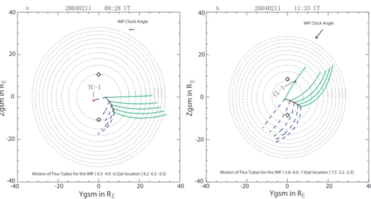
Fig. 9. Motion of reconnected flux tubes for low-latitude reconnection under IMF clock angle of (a) 85.63◦and (b) 148.13◦, respectively,
which is obtained by running the Cooling model. The reconnection conditions are satisfied along a merging line, the projection of which is indicated by the black diagonal line in the middle of the figure. The solid lines indicate the trajectories of tubes which connect to the northern cusp, and the dashed lines indicate those which connect to the southern cusp. The position of Cluster and TC-1 was represented by the blue and red star dot, respectively.
Table 1. Cataloge of Cluster FTE motion for the FTEs marked in Fig. 3, and the expected motion of the flux tubes by running the Cooling
model and the angle between the expected velocities and the Cluster observations, together with the expected motion for the two FTEs measured by TC-1. The directions (n) and the speeds (|V|)of the motion are obtained from four-spacecraft techniques, and the size of each flux tube observed by Cluster was estimated by using the velocity and the duration of the whole bipolar signature of each FTE.
FTEs UT nGSM |V| Size ExpectednGSM Expected|V| Angle
Cluster/TC-1 (motion) km s−1) (RE) (motion) (km s−1) (◦)
1 11:12:30 −0.80,0.55,0.26 100.71 1.28 −0.75,0.21,0.62 357.83 28.81
2 11:33:26 −0.84,0.27,0.45 116.48 0.79 −0.72,0.40,0.57 334.43 12.30
i 09:28:01 −0.28,−0.94,−0.19 140.41
ii 09:44:07 −0.41,−0.76,−0.51 166.68
FTEs for simplification in context, the Cooling model has still been applied. As an example, Fig. 9 presents the mo-tion of reconnected flux tubes for low-latitude reconnecmo-tion, obtained by running the Cooling model under IMF clock angle of about 85◦ (a) for TC-1 at about 09:28 UT (lagged time) and about 148◦ (b) for Cluster at about 11:33 UT (lagged time). In Fig. 9a, the corresponding input param-eters are: NSW=7.12 cm−3, VSW=368.13 km s−1, BX=
6.50 nT, BY= −3.99 nT, BZ =0.20 nT, RBS=13.5RE, RMP=10.61RE. In Fig. 9b, the corresponding input
param-eters are: NSW=16.58 cm−3,VSW=365.39 km s−1,BX=
3.75 nT, BY= −6.02 nT, BZ= −7.59 nT, RBS=11.5RE, RMP=8.48RE. Here,NSWandVSWpresent the solar wind
number density and velocity, respectively;BX,BY,BZ are
the three components of IMF in GSM coordinates, andRBS
andRMPare the stand-off distance of bow shock and
magne-topause, respectively. The view shows the YZ plane, looking earthward from the Sun. The dotted circles indicate the ra-dius of the magnetopause at X coordinate intervals 5RE. The
innermost circle representsX=(1/2)RMP and contains the
1000 ms
-9
3 15
09:30:00 -09:32:00
11 Feb 2004 +Z(5 nT)
+Y
(-68 min)
N a3
-1
100 200 300 400 500 600 700 800 900 1000
Velocity (ms-1)
0
-9 3
15 09:34:00
-09:36:00
11 Feb 2004 +Z(5 nT)
+Y (-69 min) 1000 ms N a4 -1 -9 -9 3 15 15 09:36:00 -09:38:00
11 Feb 2004 +Z(5 nT)
+Y (-68 min) 1000 ms N a5 -1 09:22:00 -09:24:00 11 Feb 2004
+Z(5 nT) +Y (-68 min) HAN 1000 ms N a1 -1 3 3 09:26:00 -09:28:00
11 Feb 2004 +Z(5 nT)
+Y (-68 min) 1000 ms N a2 -1 -9 3 3 09:46:00 -09:48:00 11 Feb 2004
+Z(5 nT) +Y (-70 min) 1000 ms N a7 -1 -9 3 15 09:40:00 -09:42:00
11 Feb 2004 +Z(5 nT)
+Y (-69 min) 1000 ms N a6 -1 1000 ms -21 -9 3 3 09:26:00 -09:28:00
11 Feb 2004 +Z(5 nT)
+Y (-68 min) S b2 -1 1000 ms -21 -9 3 09:30:00 -09:32:00 11 Feb 2004
3
+Z(5 nT)
+Y
(-68 min)
S b3
-1
-21 -9 3
09:34:00 -09:36:00
11 Feb 2004 +Z(5 nT)
+Y (-69 min) 1000 ms S b4 -1 -21 -9 09:36:00 -09:38:00
11 Feb 2004 +Z(5 nT)
+Y (-68 min) 1000 ms S b5 -1 -21 -9 3 09:40:00 -09:42:00
11 Feb 2004 +Z(5 nT)
+Y (-69 min) 1000 ms S b6 -1
-21 -93 15 09:46:00
-09:48:00
11 Feb 2004 +Z(5 nT)
+Y (-70 min) 1000 ms S b7 -1 1000 ms 09:22:00 -09:24:00
11 Feb 2004 +Z(5 nT)
+Y (-68 min) S b1 -1 KER 9:22 9:24 9:26 9:28 9:30 9:32 9:34 9:36 9:38 9:40 9:42 9:44 9:46 300 500 700 900 1100
Northern Hemisphere Southern Hemisphere c -1 Velocity at ‘ ’ (ms )
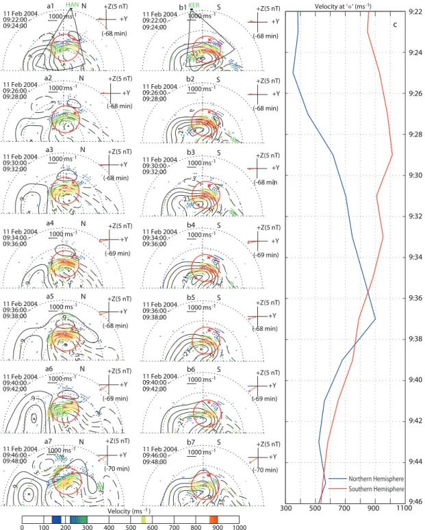
Fig. 10. Streamlines and vectors of the dayside ionospheric flows derived from the Northern (a1–7 and d1–6) and Southern (b1–7 and
d1 N
11:18:00 -11:20:00
11 Feb 2004 +Z (5 nT)
+Y
(-69 min)
HAN
1000 ms-1
-33 -21 -9 3 3 15 11:36:00 -11:38:00
11 Feb 2004 +Z (5 nT)
+Y
(-70 min)
1000 ms-1
d4 N -45 -33 -21 -9 3 3 3 15 11:42:00 -11:44:00
11 Feb 2004 +Z (5 nT)
+Y
(-68 min)
1000 ms-1
d5 N -45 -33 -21 -21 -9 3 3 11:48:00 -11:50:00
11 Feb 2004 +Z (5 nT)
+Y
(-69 min)
1000 ms-1
d6 N -33 -21 -9 3 15 11:30:00 -11:32:00
11 Feb 2004 +Z (5 nT)
+Y
(-69 min)
1000 ms-1
d3 N -21 -9 3 15 11:24:00 -11:26:00
11 Feb 2004 +Z (5 nT)
+Y
(-70 min)
1000 ms-1
d2 N
100 200 300 400 500 600 700 800 900 1000
Velocity (ms-1)
0
11:18:00 -11:20:00 11 Feb 2004
1000 ms-1
KER
+Z (5 nT)
+Y
(-69 min)
e1 S
1000 ms-1
-21 -9 3 3 3 15 15 11:24:00 -11:26:00
11 Feb 2004 +Z (5 nT)
+Y
(-70 min)
e2 S
1000 ms-1
-21
-9
3 3 15 15
11:30:00 -11:32:00
11 Feb 2004 +Z (5 nT)
+Y (-69 min) e3 S -21 -9 3 3 15 11:36:00 -11:38:00
11 Feb 2004 +Z (5 nT)
+Y (-70 min) e4 S -33 -21 -9 3 3 3 15 11:42:00 -11:44:00
11 Feb 2004 +Z (5 nT)
+Y (-68 min) e5 S -45 -33 -21 -9 -9 3 3 15 11:48:00 -11:50:00 11 Feb 2004
+Z (5 nT)
+Y
(-69 min)
e6 S
1000 ms-1
1000 ms-1
1000 ms-1
11:18 11:20 11:22 11:24 11:26 11:28 11:30 11:32 11:34 11:36 11:38 11:40 11:42 11:44 11:46 11:48 300 350 400 450 500 550 600 650 700 750
-1
Northern Hemisphere Southern Hemisphere
f
Velocity at ‘ ’ (ms )
Fig. 10. Continued.
Table 2. The IMF and solar wind conditions at the core time of FTE i observed by TC-1 and the FTE 6 measured by Cluster on 11
Febru-ary 2004, and of the 12:31 UT FTE and 12:51 UT FTE on 1 April 2004 (reported by Zhang et al., 2008).
IMF and Solar Wind FTEs on 11 February 2004 FTEs on 1 April 2004
FTE i FTE 6 12:31 UT FTE 12:51 UT FTE
BX(nT) 6.3 3.9 −2.6 −2.4
BY(nT) −4.1 −4.5 2.2 3.2
BZ(nT) −0.6 −9.3 −2.5 −1.4
Clock Angle (◦) 94.4 154.4 138.7 108.7
Elevation Angle (◦) −84.6 −22.7 46.1 59.7
Cone Angle (◦) 33.3 69.3 128.0 124.5
in the middle of the figure, where its length has been limited to an arbitrary maximum of 10REand the model allows the
position relative to the subsolar point to be chosen. Pairs of open reconnected flux tubes are assumed to be initiated along the merging line and are followed over a period of 600 s, re-sulting in the fan of motion tracks shown. The trajectories of flux tubes which connect to the northern cusp are indi-cated by the solid lines and the dashed lines indicate those which connect to the southern cusp. The positions of TC-1 and Cluster S/C 1 are represented by the red and blue star dots in Fig. 9a and b, respectively. It is clear from the chang-ing IMF direction that both spacecraft may observe a variety of FTE motions depending on the different IMF conditions, which agrees well with the results of Dunlop et al. (2005) and Zhang et al. (2008).
We show the expected velocities of the flux tubes near the spacecraft corresponding to the two FTEs observed by Cluster and the angle between the expected (Cooling) veloc-ities and the Cluster observations in Table 1. These results demonstrate that the expected motion is mainly northeast. The speeds of the expected flux tubes are∼358 km s−1and 334 km s−1, and the angles are all less than 30◦. This sug-gests that the direction of motion of the expected flux tube are relatively consistent with that of the FTEs observed by Clus-ter, but the predicted speeds are a factor of two to three times higher than the Cluster observations, which is roughly con-sistent with the statistical results of Fear et al. (2007). This might also be caused by the following two reasons. Firstly, the velocity derived from the four-spacecraft techniques is the velocity of the FTE perpendicular to the flux tube, and the axis is assumed to extend infinitely, so motion along the FTE axis cannot be estimated. Secondly, the motion of a flux tube branch at positions further from the point at which it threads the magnetopause may be more influenced by lo-cal magnetosheath flows (Fear et al., 2007). The expected (Cooling) velocities of the flux tubes, corresponding to TC-1 observations, are also presented in Table 1, and show that the expected motion is southwest. The speeds of the expected flux tubes are∼140 km s−1and 167 km s−1, respectively.
3.2 Ionospheric convection
The motion of individual flux tubes may be expected to cor-respond to the local motion in the ionospheric flow cells at their footprints and it is interesting to briefly examine the global ionospheric convection observed by SuperDARN radars in both hemispheres in this context, which will help us to understand how the high-latitude ionospheric convec-tion responds to a change in reconnecconvec-tion rate and/or locaconvec-tion such as it occurs when a change in the IMF orientation im-pacts the magnetopause. We therefore present the two minute averaged dayside ionospheric convection patterns observed by the SuperDARN radar in Fig. 10. An increasing clock an-gle should result in an ionospheric convection flow enhance-ment (Lockwood et al., 2003) and the observed flow cells
show sensitivity to the IMF orientation in this sequence also. The SuperDARN radars also provide a unique way to directly monitor two-dimensional convection in the high-latitude ionosphere on a global scale. We therefore also present the ionospheric convection patterns with the map po-tential plots, derived by using the technique of Ruohoniemi and Baker (1998), observed by nine of the Northern Hemi-sphere radars and four of the Southern HemiHemi-sphere radars during the interval of interest.
The panels in Fig. 10 show successive flow maps for the Northern and Southern Hemisphere from 09:22 to 09:46 UT (a1–7 and b1–7) and from 11:18 to 11:48 UT (d1–6 and e1– 6), in order to correspond closely to the highlighted FTE i observed by TC-1 and FTE 2 measured by Cluster, respec-tively. The dashed concentric circles indicate lines of con-stant magnetic latitude in 10◦increments and noon is located
at the top of each plot. The cross-hair axis inset at the top right of each plot shows the IMFBY and BZ components
as a red arrow, where the time delay from ACE to the iono-sphere is also indicated. The red circle highlights the region of velocity enhancement, as indicated by increased lengths of color drift vectors. The red star and blue circle represents the ionospheric footprint of TC-1 (in Fig. 10a1–7 and Fig. 10b1– 7) and of Cluster S/C 1 (in Fig. 10d1–6), respectively. The field-of-view of the CUTLASS Finland radars (HAN) and Kerguelen radar (KER) is presented as a fan in Fig. 10a1 (d1) and b1 (e1), respectively. The violet line in each fan represents the open-closed boundary (OCB), marked by the Doppler spectral width boundary from each beam (Baker et al., 1995, 1997; Chisham et al., 2001, 2005). We note that the footprint of TC-1 or Cluster lie slightly equatorward of the OCB and are out of the flow burst region. This is be-cause the TC-1 or Cluster position lies on magnetospheric field lines computed from the Tsyganenko’ 96 model, rather than at the boundary, and therefore that the computed foot-prints lie slightly equatorward of the likely true locations. These points suggest that these FTEs have motions, which reflect the likely flow directions at the respective poleward positions of their footprints (e.g. the position at the violet circle in Fig. 10a and b and the violet rhombus in Fig. 10d and e). The convection cell pattern implies a relatively direct global context for the evolution of the sampled FTEs. The time series of ionospheric flow velocity, which are extracted from the convection maps at the violet circle in Fig. 10a and b and the violet rhombus in Fig. 10d and e, are presented in Fig. 10c and f, respectively, where the time is selected the middle time of each pattern.
the Northern and Southern Hemisphere in Fig. 10 (a2–6 and b2–6, morning cell) and in Fig. 10 (d2–5 and e2–4, afternoon cell). The velocity enhancements lasted about 18–22 min for both the FTE i observed by TC-1 and the FTE 2 measured by Cluster, which might suggest that the evolution time of FTEs is about 18–22 min from their origin on magnetopause (at reconnection site) to their addition to the magnetotail lobe. These are roughly consistent with the expected ionospheric flow excitation and decay time scale of 10–15 min (Cowley and Lockwood, 1992). These correspond to the ionospheric response to the FTE i observed by TC-1 and FTE 2 measured by Cluster. Near the positions of the violet circle, the drift vectors are mainly in westward (eastward) in the Southern (Northern) Hemisphere, in a good agreement with the expec-tations from the Cooling analysis; and near the violet rhom-bus, the drift vectors are mainly in northward to northeast in the Northern Hemisphere, also in a good agreement with the expectations from the Cooling analysis and the Cluster obser-vations. The correspondence with the convection signatures confirms that individual flux tube movements are consistent with the anti-sunward ionospheric convections in the cusp re-gions of both hemispheres, and therefore are consistent with the two-dimensional (2-D) reconnection pulse model (Saun-ders et al., 1983; Southwood et al., 1988), where the model explains the bulge as the effect of a pulse of enhanced recon-nection rate at an X-line whose length is not specified and allows for longitudinal event elongation. As this model pre-diction, the footprint of the newly opened flux tube moves along the streamlines in the distorted “two-cell” convection pattern, and the ionospheric signatures of these events show that patches of newly opened flux, produced by successive reconnection pulses, are appended to each other in a contigu-ous manner, causing discontinucontigu-ous steps in the cusp ion dis-persion on the boundaries between poleward moving events (Lockwood and Hapgood, 1998). This correspondence (with the conjugate response) confirms the interpretation from the analysis in Sect. 2, despite the lack of direct one-to-one iden-tifications with the ionospheric FTE signatures. These com-parisons further suggest the formation of an extensive, low latitude merging line, with a reconnection geometry reflected in the observed FTE motion.
Comparing the ionospheric convections in both hemi-spheres, we find the velocity enhancements starting from 09:25 and 11:23 UT in the Northern Hemisphere and from 09:23 and 11:19 UT in the Southern Hemisphere for the FTE i observed by TC-1 and the FTE 2 measured by Cluster, respectively, which suggests the ionospheric response time in the Northern Hemisphere is 2 min later for the FTE i ob-served by TC-1 and 4 min later for the FTE 2 measured by Cluster than in the Southern Hemisphere. Does this suggest the reconnection site is located southward of the subsolar re-gion? This might need better data coverage in the Southern Hemisphere to show the further evidence or be because of a different conductivity in the northern and southern high-latitude ionosphere. Whilst the intensities of the ionospheric
convections are much stronger in the Southern Hemisphere than in the Northern Hemisphere for FTE i under the con-ditions of smaller IMF clock angles (∼94.4◦, see in Table 2
and Fig. 10a), they are stronger in the Northern Hemisphere than in the Southern Hemisphere for FTE 2 under the con-ditions of larger IMF clock angles (∼154.4◦, see in Table 2 and Fig. 10b). This might lead to an unclear developing and fading of the velocity enhancement in the ionosphere of the more intense hemisphere because of the stronger background and suggests that the asymmetry of the intensities of the ionospheric convections between the Northern and Southern Hemisphere are IMF clock angle dependent. The convection signatures therefore show that there is a good response to the IMF conditions resulting in clear anti-sunward ionospheric convections at the cusp regions of both hemispheres, consis-tent with the onset of low-latitude reconnection and a pre-dominantly eastward IMF. The velocity enhancements of the ionospheric convections, corresponding to the other FTEs, show the similar character, although they are not so strong and clear.
It is worth noting that the implied evolution time of these FTEs are different with the results reported by our previ-ous paper (Zhang et al., 2008), but the response time of these FTEs are similar. That paper showed that the im-plied evolution time of the FTEs was about 4–6 min from its origin on magnetopause (at reconnection site) to its ad-dition to the polar cap (the magnetotail lobe), and the iono-spheric response time in the Southern Hemisphere were 2– 6 min longer than that in the Northern Hemisphere for the events on 1 April 2004. This might be because of the dayside magnetopause reconnection occurred at the different hemi-sphere and the FTEs had different speed under the differ-ent IMF and solar wind conditions (see Table 2). From Table 2, we can find that for the two FTEs on 11 Febru-ary 2004, the IMF had negative BY and BZ with a
posi-tiveBXcomponent, giving a negative elevation angle
(eleva-tion angle = (BX/|BX|)tan−1(|BX|/BZ))and a smaller cone
angle (cone angles = cos−1(BX/|B|)); for the two FTEs on
1 April 2004 (reported by Zhang et al., 2008), the IMF had negativeBXandBZwith a positiveBYcomponent, giving a
positive elevation angle and a larger cone angle. Consider-ing the topology of Earth magnetic field durConsider-ing each event, the negative (positive) elevation angle and/or smaller (larger) cone angle with a negative (positive) BY component may
suggest the reconnection site is located southward (north-ward) of the subsolar region. This is because the first con-tact point between IMF and Earth’s magnetic field at day-side magnetopause (largest shear angle point) will be lo-cated at southward (northward) of the subsolar region when the IMF BX component is positive (negative) with a
neg-ative BZ. The solar wind speeds are smaller for the two
4 Summary
In summary, we have presented the features of two FTEs ob-served by TC-1 and two FTEs measured by Cluster, while the Cluster array was near the high-latitude magnetopause and the TC-1 spacecraft was near the subsolar magnetopause. The ionospheric plasma flow and convection analysis, which are simultaneously observed by the ESR and CUTLASS Fin-land and Kerguelen SuperDARN radar, and conjugate ob-served by the SuperDARN radars, are also presented and support well the in-situ observations. Using the Cluster 4-spacecraft observations, we calculated the velocity and the size of the flux tubes. The inferred northwardly (south-wardly) reconnected flux tubes for these FTEs are shown to move northward (southward) or north-east (south-west) and tailward, either with dominant northward (southward) or dominant eastward (westward) velocity components un-der the stable IMF and high clock angle conditions. Un-der the unstable IMF and low clock angle conditions the motion is more eastward (westward). The FTE motion is consistent with the expected motion of reconnected mag-netic flux tubes over the surface of the magnetopause, aris-ing from a predominantly subsolar reconnection site duraris-ing the prevailing IMF and solar wind conditions. The simul-taneous ESR measurements recorded poleward flow and the CUTLASS Finland and Kerguelen SuperDARN radar obser-vations showed the “poleward-moving radar auroral forms” (PMRAFs), indicative of bursty reconnection at the subso-lar region of magnetopause and the simultaneous and conju-gate SuperDARN observations show that flux tube motion is consistent with global conjugate ionospheric convections in both hemispheres. The flux tube footprints map to clear posi-tions in a predominantly two-cell convection pattern, which are temporally correlated with the local ionospheric flow en-hancements at these positions. The time durations of the velocity enhancements in the both hemispheres might im-ply that the evolution time of FTEs is about 18–22 min from their origin on magnetopause (at reconnection site) to their addition to the magnetotail lobe. However, the ionospheric response time in the Northern Hemisphere is 2 and 4 min longer than the response time in the Southern Hemisphere, for the FTE i observed by TC-1 and the FTE 2 measured by Cluster, respectively.
Acknowledgements. This work is supported by the National Natu-ral Science Foundation of China (grant No. 41104091, 41031064, 40890164, 40974083), the Natural Science Foundation of Shanghai, China (grant No. 11ZR1441200), the Youth Scientific and Techno-logical Innovation Foundation, Polar Research Institute of China (No. JDQ201001) and Ocean Public Welfare Scientific Research Project, State Oceanic Administration People’s Republic of China (No. 201005017). M. W. Dunlop is partly supported by Chinese Academy of Sciences (CAS) visiting Professorship for senior in-ternational scientists (Grant No. 2009S1-54). M. Lester is sup-ported by STFC grant ST/H002480/1. We acknowledge the NASA CDAWeb site to supply us the solar wind and IMF data from the
ACE spacecraft. We thank the Cluster/Double Star Operations
Teams, the Cluster FGM PI, E. A. Lucek and the TC-1 FGM PI C. M. Carr for the magnetic field data, the Cluster/Double Star PEACE PI A. N. Fazakerley, for the electron spectrometer data, and the Cluster CIS PI H. R`eme, for the ions data.
Guest Editor A. Masson thanks two anonymous referees for their help in evaluating this paper.
References
Amm, O., Donovan, E. F., Frey, H., Lester, M., Nakamura, R., Wild, J. A., Aikio, A., Dunlop, M., Kauristie, K., Marchaudon, A., Mc-Crea, I. W., Opgenoorth, H.-J., and Strømme, A.: Coordinated studies of the geospace environment using Cluster, satellite and ground-based data: an interim review, Ann. Geophys., 23, 2129– 2170, doi:10.5194/angeo-23-2129-2005, 2005.
Balogh, A., Carr, C. M., Acu˜na, M. H., Dunlop, M. W., Beek, T. J., Brown, P., Fornacon, H., Georgescu, E., Glassmeier, K.-H., Harris, J., Musmann, G., Oddy, T., and Schwingenschuh, K.: The Cluster Magnetic Field Investigation: overview of in-flight performance and initial results, Ann. Geophys., 19, 1207–1217, doi:10.5194/angeo-19-1207-2001, 2001.
Baker, K. B., Dudeney, J. R., Greenwald, R. A., Pinnock, M., Newell, P. T., Rodger, A. S., Mattin, N., and Meng, C.-I.: HF radar signatures of the cusp and low-latitude boundary layer, J. Geophys. Res., 100, 7671–7695, 1995.
Baker, K. B., Rodger, A. S., and Lu, G.: HF-radar observations of the dayside magnetic merging rate: A Geospace Environment Modeling boundary layer campaign study, J. Geophys. Res., 102, 9603–9617, 1997.
Berchem, J. and Russell, C. T.: Flux transfer events on the magne-topause: Spatial distribution and controlling factors, J. Geophys. Res., 89, 6689–6703, 1984.
Carr, C., Brown, P., Zhang, T. L., Gloag, J., Horbury, T., Lucek, E., Magnes, W., O’Brien, H., Oddy, T., Auster, U., Austin, P., Ay-dogar, O., Balogh, A., Baumjohann, W., Beek, T., Eichelberger, H., Fornacon, K.-H., Georgescu, E., Glassmeier, K.-H., Ludlam, M., Nakamura, R., and Richter, I.: The Double Star magnetic field investigation: instrument design, performance and high-lights of the first year’s observations, Ann. Geophys., 23, 2713– 2732, doi:10.5194/angeo-23-2713-2005, 2005.
Chisham, G., Pinnock, M., and Rodger, A. S.: The response of the HF radar spectral width boundary to a switch in the IMF By direction: Ionospheric consequences of transient dayside recon-nection? J. Geophys. Res., 106, 191–202, 2001.
Chisham, G., Freeman, M. P., Sotirelis, T., Greenwald, R. A., Lester, M., and Villain, J.-P.: A statistical comparison of Su-perDARN spectral width boundaries and DMSP particle precip-itation boundaries in the morning sector ionosphere, Ann. Geo-phys., 23, 733–743, doi:10.5194/angeo-23-733-2005, 2005. Chisham, G., Lester, M., Milan, S. E., Freeman, M. P., Bristow, W.
Cooling, B. M. A., Owen, C. J., and Schwartz, S. J.: Role of the magnetosheath flow in determining the motion of the open flux tubes, J. Geophys. Res., 106, 18763–18775, 2001.
Cowley, S. W. H. and Lockwood, M.: Excitation and decay of so-lar wind-driven flows in the magnetosphere-ionosphere system, Ann. Geophys., 10, 103–115, 1992.
Daly, P. W., Williams, D. J., Russell, C. T., and Keppler, E.: Particle signature of magnetic flux transfer events at the magnetopause, J. Geophys. Res., 86, 1628–1632, 1981.
Dungey, J. W.: Interplanetary magnetic field and the auroral zones, Phys. Rev. Lett., 6, 47–48, 1961.
Dunlop, M. W., Balogh, A., Cargill, P., Elphic, R. C., Fornaon, K.-H., Georgescu, E., Sedgemore-Schulthess, F., and the FGM team: Cluster observes the Earth’s magnetopause: coordinated four-point magnetic field measurements, Ann. Geophys., 19, 1449–1460, doi:10.5194/angeo-19-1449-2001, 2001.
Dunlop, M. W., Taylor, M. G. G. T., Davies, J. A., Owen, C. J., Pitout, F., Fazakerley, A. N., Pu, Z., Laakso, H., Bogdanova, Y. V., Zong, Q.-G., Shen, C., Nykyri, K., Lavraud, B., Milan, S. E., Phan, T. D., R`eme, H., Escoubet, C. P., Carr, C. M., Cargill, P., Lockwood, M., and Sonnerup, B.: Coordinated Cluster/Double Star observations of dayside reconnection signatures, Ann. Geo-phys., 23, 2867–2875, doi:10.5194/angeo-23-2867-2005, 2005. Elphic, R. C., Lockwood, M., Cowley, S. W. H., and Sandholt, P. E.:
Flux transfer events at the magnetopause and in the ionosphere, Geophys. Res. Lett., 17, 2241–2244, 1990.
Escoubet, C. P., Fehringer, M., and Goldstein, M.: Introduc-tion: The Cluster mission, Ann. Geophys., 19, 1197–1200, doi:10.5194/angeo-19-1197-2001, 2001.
Farrugia, C. J., Rijnbeek, R. P., Saunders, M. A., Southwood, D. J., Rodgers, D. J., Smith, M. F., Chaloner, C. P., Hall, D. S., Chris-tiansen, P. J., and Woolliscroft, L. J. C.: A multi-instrument study of flux transfer event structure, J. Geophys. Res., 93, 14465– 14477, 1988.
Fazakerley, A. N., Carter, P. J., Watson, G., Spencer, A., Sun, Y. Q., Coker, J., Coker, P., Kataria, D. O., Fontaine, D., Liu, Z. X., Gilbert, L., He, L., Lahiff, A. D., Mihalˇciˇc, B., Szita, S., Taylor, M. G. G. T., Wilson, R. J., Dedieu, M., and Schwartz, S. J.: The Double Star Plasma Electron and Current Experiment, Ann. Geo-phys., 23, 2733–2756, doi:10.5194/angeo-23-2733-2005, 2005. Fear, R. C., Fazakerley, A. N., Owen, C. J., Lahiff, A. D., Lucek,
E. A., Balogh, A., Kistler, L. M., Mouikis, C., and R`eme, H.: Cluster observations of bounday layer structure and a flux transfer event near the cusp, Ann. Geophys., 23, 2605–2620, doi:10.5194/angeo-23-2605-2005, 2005.
Fear, R. C., Milan, S. E., Fazakerley, A. N., Owen, C. J., Asikainen, T., Taylor, M. G. G. T., Lucek, E. A., Rme, H., Dandouras, I., and Daly, P. W.: Motion of flux transfer events: a test of the Cooling model, Ann. Geophys., 25, 1669–1690, doi:10.5194/angeo-25-1669-2007, 2007.
Greenwald, R. A., Baker, K. B., Dudeney, J. R., Pinnock, M., Jones, T. B., Thomas, E. C., Villain, J.-P., Cerisier, J.-C., Senior, C., Hanuise, C., Hunsucker, R. D., Sofko, G., Koehler, J., Nielsen, E., Pellinen, R., Walker, A. D. M., Sato, N., and Yamagishi, H.: Darn/SuperDARN: A global view of the dynamics of high-latitude convection, Space Sci. Rev., 71, 761–796, 1995. Haerendel, G., Paschmann, G., Sckopke, N., Rosenbauer, H., and
Hedgecock, P. C.: The frontside boundary layer of the magne-topause and the problem of reconnection, J. Geophys. Res., 83,
3195–3216, 1978.
Harvey, C. C.: Spatial gradients and the volumetric tensor, in: Anal-ysis Methods for Multi-Spacecraft Data, edited by: Paschmann, G. and Daly, P. W., pp. 307–348, ISSI, 1998.
Hasegawa, H., Sonnerup, B. U. ¨O., Owen, C. J., Klecker, B., Paschmann, G., Balogh, A., and R`eme, H.: The structure of flux transfer events recovered from Cluster data, Ann. Geophys., 24, 603–618, doi:10.5194/angeo-24-603-2006, 2006.
Johnstone, A. D., Burge, S., Carter, P. J., Coates, A. J., Coker, A. J., Fazakerley, A. N., Grande, M., Gowan, R. A., Gurgiolo, C., Hancock, B. K., Narheim, B., Preece, A., Sheather, P. H., Win-ningham, J. D., and Woodliffe, R. D.: PEACE: A plasma electron and current experiment, Space Sci. Rev., 79, 351–389, 1997. Karhunen, T. J. T., Arnold, N. F., Robinson, T. R., and Lester,
M.: Determination of the parameters of traveling ionospheric disturbances in the high-latitude ionosphere using CUTLASS coherent-scatter radars, J. Atmos. Solar Terr. Phys., 68, 558–567, 2006.
Lester, M., Chapman, P. J., Cowley, S. W. H., Crooks, S. J., Davies, J. A., Hamadyk, P., McWilliams, K. A., Milan, S. E., Parsons, M. J., Payne, D. B., Thomas, E. C., Thornhill, J. D., Wade, N. M., Yeoman, T. K., and Barnes, R. J.: Stereo CUTLASS – A new capability for the SuperDARN HF radars, Ann. Geophys., 22, 459–473, doi:10.5194/angeo-22-459-2004, 2004.
Liou, K., Newell, P. T., and Meng, C.-I.: Characteristics of the solar wind controlled auroral emissions, J. Geophys. Res., 103, 17543–17557, 1998.
Liu, Z. X., Escoubet, C. P, Pu, Z., Laakso, H., Shi, J. K., Shen, C., and Hapgood, M.: The Double Star mission, Ann. Geophys., 23, 2707–2712, doi:10.5194/angeo-23-2707-2005, 2005.
Lockwood, M.: Flux-transfer events at the dayside magnetopause – transient reconnection or magnetosheath dynamic pressure pulses?, J. Geophys. Res., 96, 5497–5509, 1991.
Lockwood, M. and Carlson, H. C.: Production of polar cap electron density patches by transient magnetopause reconnection, Geo-phys. Res. Lett., 19, 1731–1734, 1992.
Lockwood, M. and Hapgood, M. A.: On the Cause of a Magne-tospheric Flux Transfer Event, J. Geophys. Res., 103, 26453– 26478, 1998.
Lockwood, M. and Smith, M. F.: The variation of reconnection rate at the dayside magnetopause and cusp ion precipitation, J. Geo-phys. Res., 97, 14841–14847, 1992.
Lockwood, M. and Wild, M. N.: On the quasi-periodic nature of magnetopause flux-transfer events, J. Geophys. Res., 98, 5935– 5940, 1993.