Multi-spacecraft observation of plasma dipolarization/injection in the inner magnetosphere

www.ann-geophys.net/25/801/2007/ © European Geosciences Union 2007

Annales

Geophysicae

Multi-spacecraft observation of plasma dipolarization/injection in

the inner magnetosphere

S. V. Apatenkov1, V. A. Sergeev1, M. V. Kubyshkina1, R. Nakamura2, W. Baumjohann2, A. Runov2, I. Alexeev3, A. Fazakerley3, H. Frey4, S. Muhlbachler5, P. W. Daly5, J.-A. Sauvaud6, N. Ganushkina7, T. Pulkkinen7, G. D. Reeves8, and Y. Khotyaintsev9

1_{Institute of Physics, St. Petersburg State University, St. Petersburg, Russia} 2_{Space Research Institute, Austrian Academy of Sciences, Graz, Austria} 3_{Mullard Space Science Laboratory, University College London, UK} 4_{Space Science Laboratory, Berkeley, USA}

5_{Max Planck Institute for Solar System Research, Katlenburg-Lindau, Germany} 6_{Centre d’Etude Spatiale des Rayonnements, Toulouse, France}

7_{Finnish Meteorological Institute, Helsinki, Finland} 8_{Los Alamos National Laboratory, USA}

9_{Swedish Institute of Space Physics, Uppsala, Sweden}

Received: 22 September 2006 – Revised: 23 January 2007 – Accepted: 27 February 2007 – Published: 29 March 2007

Abstract. Addressing the origin of the energetic parti-cle injections into the inner magnetosphere, we investi-gate the 23 February 2004 substorm using a favorable con-stellation of four Cluster (near perigee), LANL and Geo-tail spacecraft. Both an energy-dispersed and a disper-sionless injection were observed by Cluster crossing the plasma sheet horn, which mapped to 9–12RE in the

equa-torial plane close to the midnight meridian. Two associated narrow equatorward auroral tongues/streamers propagating from the oval poleward boundary could be discerned in the global images obtained by IMAGE/WIC. As compared to the energy-dispersed event, the dispersionless injection front has important distinctions consequently repeated at 4 space-craft: a simultaneous increase in electron fluxes at energies

∼1..300 keV,∼25 nT increase inBZand a local increase by

a factor 1.5–1.7 in plasma pressure. The injected plasma was primarily of solar wind origin. We evaluated the change in the injected flux tube configuration during the dipolarization by fitting flux increases observed by the PEACE and RAPID instruments, assuming adiabatic heating and the Liouville theorem. Mapping the locations of the injection front de-tected by the four spacecraft to the equatorial plane, we es-timated the injection front thickness to be ∼1RE and the

earthward propagation speed to be ∼200–400 km/s (at 9– 12RE). Based on observed injection properties, we

sug-gest that it is the underpopulated flux tubes (bubbles with Correspondence to:S. V. Apatenkov

([email protected])

enhanced magnetic field and sharp inner front propagating earthward), which accelerate and transport particles into the strong-field dipolar region.

Keywords. Magnetospheric physics (Energetic particles, trapped; Magnetotail; Plasma convection)

1 Introduction

Energetic particle injections (EPI) have been observed and investigated since the first high altitude spacecraft measure-ments in the inner magnetosphere (e.g. Arnoldy and Chan, 1969). EPI, sharp increases of energetic (tens-hundreds keV) particle flux, are categorized either as energy-dispersed or dispersionless events. In the latter case particle flux increases occur within 1 min for different energies. Late arrival of par-ticles with lower energy inherent to the dispersed events is explained by the azimuthal magnetic drift from the injec-tion place (eastward for electrons, westward for ions), as the velocity is proportional to both the particle energy and the magnetic field gradient; the time of flight effects are negli-gible for>50 keV particles. The dispersionless character is explained by the spacecraft being inside the injection region. Long-term continuous observations at geostationary orbit (at 6.6RE distance) showed the correlation of EPI occurrence

0 -5 -10 -15 X gsm, Re

-5 0 5

Z g

s

m

, R

e

Geotail

GOES12 LANL90

IMAGE

2004/02/23 3:20-3:30UT XZgsm plane, field lines T89, Kp=0 L095 - 0.5MLT; GOES-12 - 22MLT;

Cluster - 0.8MLT; Geotail - 00MLT

Cluster

-500 0 500

ΔX, km -500

0 500

Δ

Y

, km

-500 0 500

ΔX, km -500

0 500

Δ

Z

, km

-500 0 500

ΔY, km -500

0 500

Δ

Z

, km

C1

C3

C2

C4

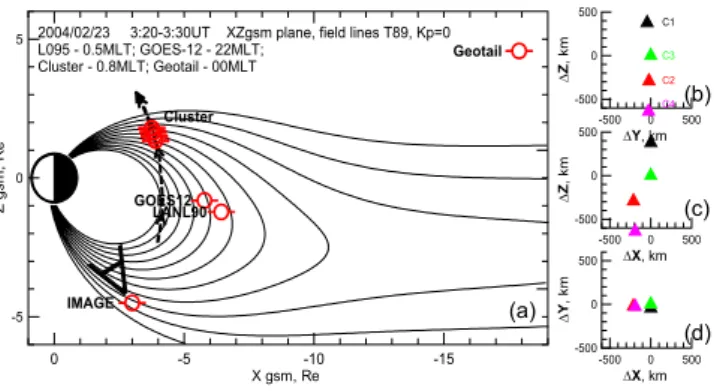
Fig. 1. (a)Spacecraft locations in theXZGSMprojection, (b–d)

zoomed-in Cluster XY,XZ,YZ projections show the pearl-on-string configuration.

recorded the earthward propagation of the dispersionless in-jections with velocities of 10–100 km/s (Moore et al., 1981; Reeves et al., 1996; Sergeev et al., 1998). Earthward veloci-ties of∼100–200 km/s at 8–9RE of the magnetic field

dipo-larization front were documented by Ohtani (1998). The azimuthal extent of the injections is typically about 1–2 lo-cal hours, i.e. 2–4RE (Reeves et al., 1991; Thomsen et al.,

2001).

One of the basic questions concerns the origin of the dis-persionless injections observed at geostationary and deeper where the gradient drifts are very strong. A successful model explaining the observed spectra was suggested by Li et al. (1998) and further developed by Sarris et al. (2002) and Zaharia et al. (2004). They traced particle trajecto-ries and estimated energization gained by the particles in the case of the earthward propagating localized structure, an electromagnetic (EM) pulse, which contained an enhanced duskward electric field and its self-consistent magnetic field variation (enhanced BZ component). Particles, which are

transported inside the EM pulse proper during some time, are less affected by the gradient drift that allows them to be injected deeper into the strong magnetic field. This model succeeded in reproducing both observed accelerated fluxes and their dispersionless character (Li et al., 2003). An im-portant requirement for the pulse parameters in these mod-els is a slow (several tens–few hundreds km/s) propagation speed. Such velocities are confirmed by some observations (e.g.∼24 km/s on average at around 6.6REby Reeves et al.,

1996;∼20 km/s at 5–6REby Sergeev et al., 1998), although

there are no such slow MHD waves in those regions, where the magnetosonic wave speed is of the order of 1000 km/s. It is only seldom when the opportunity arises to have both com-prehensive field and particle observations in the inner magne-tosphere (GOES measures only the magnetic field while the LANL instrument suite measures only particles). This makes it difficult to prove the EM pulse model observationally, es-pecially as the injection propagation (direction and velocity)

is difficult to evaluate using single spacecraft data. There is still a great need to obtain a comprehensive description of particle and field signatures of dispersionless injections with the proper distinction between temporal and spatial varia-tions. This is now possible using the four Cluster spacecraft. In this paper we study both energy dispersed and dis-persionless injections observed by the four Cluster space-craft near perigee during one favorable event. Taking advan-tage of a well-instrumented multi-spacecraft mission, com-plemented by data from other spacecraft, we (1) describe the specific properties of dispersionless injections as com-pared to energy-dispersed ones; (2) show that the dispersion-less injection corresponds to a localized spatial structure and estimate its front thickness and propagation speed; (3) per-form adiabatic heating calculations to describe the observed electron acceleration and specify the magnetospheric config-uration changes associated with a localized injection. Based on the observed injection properties we discuss bursty bulk flows (BBFs) in the magnetotail as the “vehicle” transport-ing energetic particles into the inner magnetosphere and as a candidate mechanism to produce dispersionless injections.

2 Observations

2.1 Spacecraft configuration and instruments

We start by showing the spacecraft configuration during the period of interest, 23 February 2004, at around 03:27 UT in Fig. 1. Only the projection into theXZGSM plane is pre-sented, as all spacecraft reside close to the midnight merid-ian. Magnetic field lines, according to the Tsyganenko (1989) (T89) model withKp=0, are added for reference. The

geostationary satellite GOES-12 (hereafter G12) providing

∼0.5 s resolution magnetometer data was located at about 22:00 MLT. Another geostationary spacecraft, LANL1990-095 (hereafter LLANL1990-095), was at ∼0.5 MLT and provided en-ergetic particle (electrons and protons E>50 keV) measure-ments from the SOPA instrument (see Belian et al. (1992) for the instrument description). Geotail was in the northern lobe at∼7RE above the neutral sheet (at [−17.8, 0.5, 4.6]RE

in GSM coordinates). Southern Hemisphere auroras with a 2-min resolution were observed by the IMAGE spacecraft.

The Cluster quartet had just passed the perigee and was in a pearl-on-string configuration crossing the plasma sheet horns at 0.8 MLT, as illustrated in Fig. 1. The four spacecraft followed each other, moving in the positiveZGSMdirection (Figs. 1b, c, d). In terms of the equatorial projection, the Cluster spacecraft moved from the inner magnetosphere out-ward into the plasma sheet. Independent of the external field model and mapping, C4 was the innermost spacecraft, while C1 was the most tailward spacecraft. The in-situ distance be-tween the leading (C1) and the trailing (C4) spacecraft was

A suite of Cluster instruments was used in this study. The magnetic field with a 1-s resolution was available from the FGM fluxgate magnetometer (Balogh et al., 2001). The fluxes of electrons and protons in the energy range 30– 300 keV, divided into 8 energy channels, were recorded by the RAPID instrument (Wilken et al., 2001). Lower energy 0.036–24 keV electron fluxes detected by PEACE were avail-able every spin (4 s) with 7.5deg pitch angle resolution (we use 2-D distributions) in 28 energy channels (Johnstone et al., 1997). We also used low energy (<35 keV) ion observa-tions from the CIS instrument (R`eme et al., 2001) to estimate plasma pressure and composition change, as well as the elec-tric field from the double probe EFW instrument described in Gustafson et al. (2001).

2.2 23 February 2004 event overview

According to Advanced Composition Explorer (ACE) obser-vations (Figs. 2a, b), the solar wind dynamic pressure and bulk velocity were close to their statistical average values,

∼2.5 nPa and ∼420 km/s, respectively; the IMF BZ

com-ponent varied around zero not exceeding 6 nT in absolute value. The solar wind parameters are time-shifted to the magnetopause at X=10RE, using the observed solar wind

speed VX. The BZ excursion to negative values during

01:00–02:45 UT caused enhanced magnetic flux loading into the magnetosphere and the small substorm commencing at

∼02:20 UT.

A moderate substorm started at ∼02:20 UT as the on-set of the negative bay in the magnetic X component reg-istered at the auroral station Narsarssuaq at 23:00 MLT. Sit-uated in the lobe, Geotail observed that the unloading had started at∼02:15 UT and lasted until 03:30 UT. Geostation-ary L095 registered a sequence of injections which followed the dropout at∼02:00 UT, Fig. 2d. G12 located at 21 MLT observed a smooth dipolarization starting at∼02:22 UT.

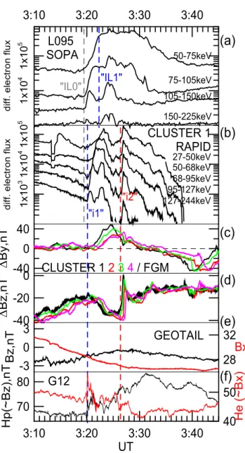
The time period of interest 03:15–3:30 UT is characterized by modest geomagnetic activity with AE=200–300 nT. The Dst index was also quiet, reaching its minimum of−11 nT at 03:00 UT. The substorm activation at∼03:15 UT is seen in Fig. 2 as the AE increase followed by particle injections. 2.3 Energetic particle injections at Cluster and L095 The Cluster quartet observed two separate energetic particle flux increases (EPIs) at∼03:20 UT and∼03:27 UT, here-after “i1” and “i2”, Fig. 3b. Both injections were observed by all four Cluster spacecraft (only Cluster 1 data are shown in Fig. 3b). L095, located deeper and westward as com-pared to Cluster, observed two separate injections: “il0” at

∼03:19 UT and “il1” at∼03:23 UT, Fig. 3a.

The injection “il0” was the first injection. “il0” was al-most dispersionless, its soft spectrum (alal-most no flux in-crease at E>150 keV) distinguishes “il0” from the following injections. The next injection, “i1” at Cluster, marked by the

0:00

1:00

2:00

3:00

4:00

UT

-5

0

5

B,

Bz,

nT

400

450

|V|, km/s

₂

3

Pdyn, nPa

1x10

1x10

1x10

di

ff

. el

ec

tr

on f

lux

0:00

1:00

2:00

3:00

4:00

AE, nT

LANL / SOPA

500

0

Fig. 2. ACE observations in the solar wind: magnetic field –(a), velocity and pressure –(b)(shifted to X=10RE). Preliminary AE index(c)and energetic electron fluxes at L095(d)are also shown. The period of interest is marked by a red bar.

blue dashed line in Fig. 3, was clearly the energy-dispersed injection. Some remnants of the earlier “il0” can be seen in low-energy channels (<68 keV) at Cluster, too. We suppose that the injection “i1” reached the geostationary orbit after a few minutes of inward propagation and was detected at L095 as the injection “il1”.

Using magnetic drift time delays for electrons of different energies we traced particles back in time and obtained an in-jection start time and MLT location (see, e.g. Reeves et al., 1991). These locations are shown by diamonds in our sum-mary diagram Fig. 5. We should note that the onsets of elec-tron flux increases could not be accurately distinguished for “i1” (low-energy channels) and “il1” due to the pre-existing background level.

At 03:20 UT, within 1 min from “il0” and “i1” detection, a sharp dipolarization front reached G12, located 2 h MLT duskward, and the dipolarization continued to progress af-terward until 03:30 UT. However, no sharp magnetic sig-natures were observed by the Cluster spacecraft related to the energy-dispersed “i1” at around 03:20 UT. The intense and smooth ∼20 min long bipolar variation in Cluster BY

-40

0

40

Δ

By,nT

3:10

3:20

3:30

3:40

UT

70

80

Hp(~

Bz),nT

-3

0

3

Bz,nT

-40

-20

0

Δ

Bz,nT

1x10

3 1x10 4 1x10

5

d

iff

. e

lec

tr

o

n

fl

u

x

1x10

4

1x10

5

di

ff

. el

ec

tr

on

f

lux

28

32

Bx

40

50

He (

~

Bx)

3:10

3:20

3:30

3:40

27-50keV

G12

GEOTAIL

CLUSTER 1

2

3

4

/ FGM

L095

SOPA

CLUSTER 1

RAPID

75-105keV

105-150keV

150-225keV

50-68keV 68-95keV 95-127keV 127-244keV

(a)

(b)

(c)

(d)

(e)

(f)

"IL0" "IL1"

"i1"

"i2"

Fig. 3. L095/SOPA energetic electrons(a), Cluster 1/RAPID(b), Cluster FGMB_Y (c);B_Z (d); GeotailB_XandB_Z magnetic field components(e); G12HpandHe(f).

the substorm current wedge eastern edge (Fig. 5); it is hardly related to the particle injections.

The dispersionless injection, “i2”, was observed at

∼03:27 UT by four Cluster spacecraft, but it probably did not reach the geostationary orbit; no injection remnants were found deeper at L095, except for a small flux increase in the 75–105 keV electron channel, Fig. 3a. A similar sharp varia-tion was observed in the magnetic field at Cluster, especially in theBZ component, which increased by 25–30 nT during

∼16 s simultaneously with the electron flux growth. A more detailed presentation of Cluster observations will be given in Sect. 3.

2.4 Global auroral observation with IMAGE/WIC

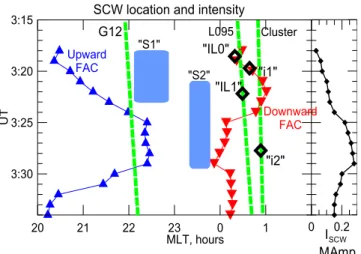
A sequence of auroral images observed by IMAGE/WIC in the Southern Hemisphere is presented in Fig. 4. The back-ground level has been removed, as the auroras were rather faint and the image was visibly affected by direct solar ra-diation. The bright “oval” visible at ∼70◦ CGLat in the dusk-midnight sector is actually only the poleward part of the auroral oval. According to the DMSP F14 flyby at 03:25–03:29 UT in the near-midnight sector, the poleward and equatorward boundaries were located at∼71.5 and 63◦ CGLat, 23:00–24:00 h MLT. Two poleward boundary inten-sifications, marked “S1” and “S2”, were detected at 03:18 and 03:22 UT. The intensification “S1” showed distinct fea-tures of an auroral tongue propagating equatorward. The au-roral tongue was most clear and intense at 03:20 UT, but its traces can be seen on the next 3 frames until 03:24 UT at around 22.5 h MLT. The second spot “S2” was weaker and patchy, close to the background level. Its remnants can be discerned until 03:30 UT at a somewhat later MLT (∼23.5). Also, this auroral feature propagated equatorward. Both in-tensifications (although rather faint in the equatorward part) resemble auroral streamers in the shape and behavior and may be associated with the electron injections “i1” and “i2”, which were observed 3–4 min after the initiation of poleward intensification at more dawnward location (Fig. 5).

2.5 Substorm current wedge dynamics

Using mid-latitude ground observations (25 INTERMAG-NET stations with magnetic latitudes between 15◦_{and 55}◦₎ we calculated the locations and intensity of the substorm cur-rent wedge (SCW) (see Sergeev et al., 1996a, for a descrip-tion of the algorithm). It started to develop at∼02:27 UT, was centered at about 23:00 MLT, and had a longitudinal width of ∼3 h in MLT (i.e. L095 was located inside the wedge while G12 was at its western edge, close to the up-ward FAC).

Fig. 4.IMAGE/WIC sequence for the interval 03:16–03:30 UT. Ionospheric footprints of G12, L095 and Cluster spacecraft are shown for reference by rectangles. Faint poleward boundary intensifications (probably streamers) developing equatorward are indicated by arrows “S1” and “S2”.

3:15

3:20

3:25

3:30

UT

SCW location and intensity

MLT, hours

20 21 22 23 0 1 0 0.2

ISCW

MAmp

G12 L095 Cluster

Downward FAC Upward

FAC

"S1"

"S2" "i1"

"i2" "IL1" "IL0"

Fig. 5. MLT locations of the SCW upward and downward field-aligned current (left) and SCW intensity in MAmps (right) obtained from analysing midlatitude perturbations. MLT locations of

geo-stationary G12, L095 and Cluster spacecraft (mapped at 7–12RE

equatorial) are presented by green lines. Locations of auroral pole-ward boundary intensifications are shown by light-blue bars. The onset times of electron injections observed by L095 and Cluster are shown by black diamonds.

3 Properties of the dispersionless injection as observed by Cluster

The dispersionless injection detected by the well-instrumented Cluster quartet near its perigee gives us a rare opportunity to describe the behavior of different plasma parameters and plasma species observed together with the field variations and to separate spatial and temporal effects.

-40

-20

0

Δ

Bz,

nT

3:26:00

3:27:00

3:28:00

UT

1x10

1x10

1x10

1x10

1x10

1x10

D

if

fer

ent

ial

el

ec

tr

on f

lux

, 1/

c

m

^

2 s

s

r k

eV

27-50 keV 50-68 keV 68-95 keV

95-127 keV

127-244 keV 20.8-26.7 keV 13.4-16.8 keV 5.5-6.9 keV 8.6-10.7 keV 3.5-4.4 keV 2.3-2.8 keV 1.5-1.8 keV

Fig. 6. Differential omni-directional electron flux variations in the

energy range 1–150 keV from RAPID and PEACE at C1(a);BZ

-40

-20

0

Δ

Bz,

nT

3:24:00 3:25:00 3:26:00 3:27:00 3:28:00 3:29:00 3:30:00

UT

P

ITC

H

A

N

G

L

E

(

180-top)

~ 1

k

e

V

~ 1

9

k

e

V

C1

C3

C2

C4

C1

C3

C2

C4

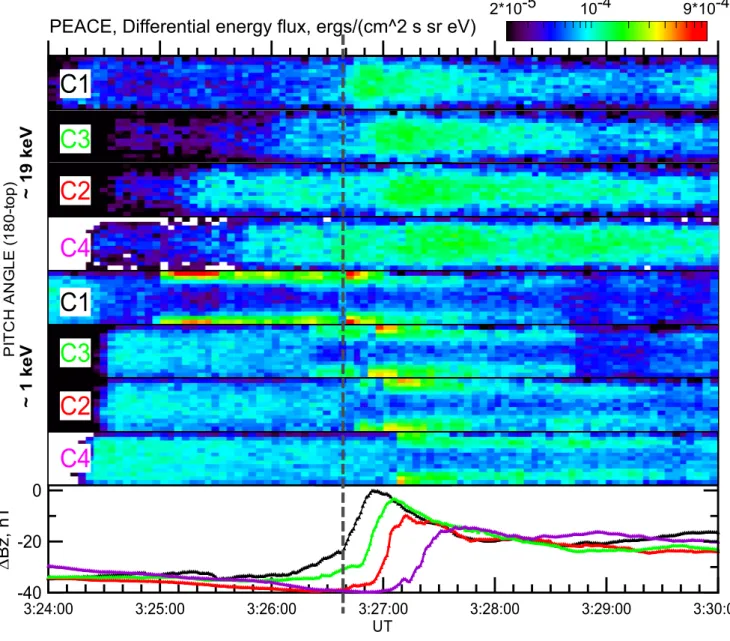
Fig. 7.Pitch-angle plots for high-energy (19 keV) and low-energy (1 keV) components from the Cluster PEACE instrument; 180◦(tailward) and 0◦(earthward) are at the top and bottom of each plot. Variations in the magnetic field are shown for reference at the bottom panel.

As shown in Sect. 2.3, the dispersionless injections at the four Cluster spacecraft were observed at the same time with the increases in theBZ magnetic component, Fig. 6. A

si-multaneous magnetic pulse and electron flux increase were repeated at all four spacecraft; thus, we can definitely as-sociate the injection signatures with a structure propagating past the spacecraft. This propagating structure has a sharp leading front that we call the injection or dipolarization front. The front passes the spacecraft in order from C1 to C4 which reveals a propagation in the negativeZGSMdirection, i.e. into the stronger dipole field considering the Cluster satellite lo-cations. The elongated tetrahedron configuration (Figs. 1b– d, Sect. 2.1) allows one only to estimate the local velocity in

the Z-direction, which was found to be∼25 km/s (Cluster or-bital motion was taken into account). Furthermore, evidence of some deceleration can be noticed. Using this speed and the 15- to 20-s duration of the leading front, we estimate its thickness to be∼450 km.

lower energies (0.1–3 keV). It was observed well before the injection at 03:25:00, 03:26:20 and 03:26:45 UT at space-craft C1, C3, and C2, respectively (C4 spacespace-craft recorded a corresponding change at around 03:27:08 UT at the injec-tion front). Based on the spacecraft locainjec-tions, this boundary seems to be a spatial boundary rather than a temporal one, the in-situ velocity was less than 2 km/s.

Secondly, two kinds of anisotropy were simultaneously observed, a field-aligned anisotropy at E<2 keV and pan-cake anisotropy at E>5 keV. To demonstrate these two dif-ferent anisotropies we present in Fig. 7 the pitch angle dis-tributions of the 1 keV and 19 keV electrons. The anisotropy character did not change during the injection front passage; the existing distributions only intensified at the front. One can notice that in all cases the fluxes of earthward low-energy electrons increase, first suggesting that the plasma fills the in-jected flux tubes in the earthward direction. A sharp change in the anisotropy at lower energies (0.1–3 keV) has been al-ready pointed out above, but it was not associated with the injection.

The low-energy ion behavior during the period of inter-est was also observed by the CIS instrument. Ion mo-ments with 8-s resolution were available from C1/HIA and C4/CODIF. The hydrogen omni-directional energy flux spec-trogram and the ion pressure from different species are pre-sented in Figs. 8a–d. The spectrogram, Fig. 8a, shows that the 5–20 keV ion population is the main contributor to the en-ergy flux, both before and during the injection. Ionospheric species He+ and O+, Fig. 8b, contribute about∼10% to the pressure while the distinct solar wind-origin ions, He++, pro-vide up to 50% of the pressure. This implies that most of the injected plasma originated from the more distant mag-netotail. We also estimated the contribution to the plasma pressure from the energetic (E>30 keV) ions and electrons using the RAPID instrument and found it to be<10% of the ion contribution measured by CIS, Figs. 8c–d. Total pressure values measured immediately before the injection by Clus-ter 1 gave about 0.4–0.5 nPa, which correspond to equato-rial radial distances of 11–12RE, according to Tsyganenko

and Mukai (2003) under the observed SW conditions (and assuming pressure isotropy). Cluster 4 measures∼0.9 nPa total pressure, which corresponds to 8–9RE equatorial

dis-tance. We note that the plasma pressure increases by a fac-tor of 1.5–1.7 at both spacecraft during the passage of the injection front (Figs. 8b–d), whether one considers the hy-drogen contribution or the total pressure. The ion velocity from C1/HIA is presented in Fig. 8e. The major variation at the front was the change in theVZGSMcomponent, which reached∼–80 km/s at its extremum. This negativeVZin situ

corresponds to an inward plasma motion, in the same direc-tion as the injecdirec-tion front propagated.

Electric field measurements (GSE X and Y components) from the EFW instrument were also available for this in-terval, amplitudes up to 40 mV/m were recorded at/near the injection front (see Fig. 9). First, we notice that variations

3:20:00

3:23:00

3:26:00

3:29:00

UT

-50

0

50

V, km/s

0.01

0.1

1

P

, nPa

0.01

0.1

1

P

, nPa

100

1000

10000

Energy, eV

0.01

0.1

P

, nPa

-40

-20

Δ

Bz,

nT

C4/CODIF

H+

He++

He+

O+

C4/RAPID, E>27keV,

H+

e-C1/RAPID, E>27keV,

H+

e-C1/HIA

Vx

Vy

Vz

C1/HIA

Fig. 8. Cluster 1 and 4 ion and energetic particle observations.

Cluster 4: (a) CIS/CODIF H+ omnidirectional energy flux; (b)

CIS/CODIF pressure with contribution from different ion species;

(c)RAPID (>27 keV) ion and electron pressure. Cluster 1: (d)

pressure contributions from CIS/HIA (black) and RAPID;(e)ion

velocity from HIA.(f)magnetic pulse in the Z component from all 4 s/c is added for reference.

in EY were dominant as compared to EY. Secondly, the

bipolar variation in EY repeated at all four s/c, Figs. 9d–

g, but the variation amplitude seems to decrease with the pulse propagation past the spacecraft. This is possibly re-lated to the braking of earthward propagation of the injected flux tube. The negativeEY pulses (corresponding to a

dawn-ward electric field) were observed first together with the on-set of sharpBZ increases. Later, still during the increasing

BZ,EY changed to positive values. The duration of the

neg-ative pulse was about 3 spacecraft spins (∼10 s). TheEY

dis-played a turbulent character right after theBZ maxima, i.e.

3:25 3:26 3:27 3:28 3:29 UT -40 -10 Δ Bz , n T -40 -10 Δ Bz , n T -20 0 20 -[VxB] Z mV /m -20 0 20 -[VxB] Y mV /m -20 0 20 EX , E Y , mV /m -40 -10 Δ Bz , n T -40 -10 Δ Bz , n T -20 0 20 EX , E Y , mV /m -20 0 20 EX , E Y , mV /m 0 20 EX , E Y , mV /m -20 0 20 -[VxB] X mV /m

ΔBz (FGM)

Ex (EFW) Ey (EFW)

E as -[VxB] E from EFW

C1

C3

C2

C4

Fig. 9. Flux transfer−[V×B]estimated from CIS/HIA and FGM observations at C1 compared with the double probeEXandEY(a–

c); EFWE_X(dashed) andE_Y electric field, together with FGMB_Z

variations at four Cluster spacecraft(d–g).

possible behavior of other E-field components we also plot-ted in Figs. 9a–c E, compuplot-ted from−[V×B]using plasma velocity from Cluster 1/HIA and B-field from FGM. It was found that (1) the X- and Y- components of −[V×B] are closely associated withEXandEY, respectively, from EFW,

and (2) the variation in the−[V×B]Y component was the

dominant component compared with the components along the tail and in north-south direction.

4 Magnetic configuration and mapping

Although Cluster provided detailed observations of the lo-calized structure associated with the dispersionless plasma injection, these observations were made in the plasma sheet horns, far from the near-equatorial region, where most of the current and magnetic field reconfiguration and plasma accel-eration took place. Therefore, we need to specify the mag-netic configuration to obtain answers to the following impor-tant questions: (a) What is the distance range (also scales and

0 -5 -10

Xgsm, Re -4 -2 0 2 Zg s m , R e T89 Kp=0 T89 Kp=1 T96 SW at 3:27 T96mod 3:24 T96mod 3:27

Cluster

GOES12

Kp=0 Kp=1

3:10 3:15 3:20 3:25 3:30 3:35 3:40

UT -40 -20 0 Δ Bz, nT -30 -20 Δ Bz, nT -5 0 Δ Bz, nT 20 30 Δ Bx, nT 20 30 Δ Bx, nT

Δ

B = B(OBS)-B(IGRF)

T89:

Kp=0;

Kp=1;

T96

(SW at 3:27);

T96mod

at 3:24UT

GOES-12 22MLT

Cluster 1 0.8MLT

Geotail 00MLT, X=-17Re

Fig. 10. Magnetic field observations at Geotail, G12, Cluster with dipole field subtracted(a–c)compared with predictions of different models T89, T96, T96mod. Magnetic field lines traced through the Cluster location using different models.

propagation speed) in the equatorial magnetosphere where the localized injection develops? (b) What is the actual geometry change in the earthward contracting plasma tube which contained the accelerated plasma? To specify the mag-netic configuration preceeding the injection we should first consider the magnetic field perturbations observed by Clus-ter, by Geotail (in the lobes at 17RE) and by GOES-12 (3 h

IGRF field subtracted) in Fig. 10, together with the magnetic fields predicted by the T89 and T96 models. Also the ob-served magnetic field values were used to tune the parameters of the T96 model (by varying the intensity of the tail current and ring current systems to obtain the best fit to the observa-tions; see Kubyshkina et al. (1999) for the method descrip-tion). This best fit model (the diamonds T96mod in Fig. 10) for 03:24 UT provides nearly the same magnetic field and similar Cluster field line shape as theKp=1 T89 model does.

According to these comparisons, the tail configuration before the injection (at the state 1) is only moderately stretched, and the equatorial crossing distance of the Cluster field line is between 10 and 13REfor the best-fit models (Fig. 10). This

method cannot, however, be applied to specify the final state of the injected flux tube.

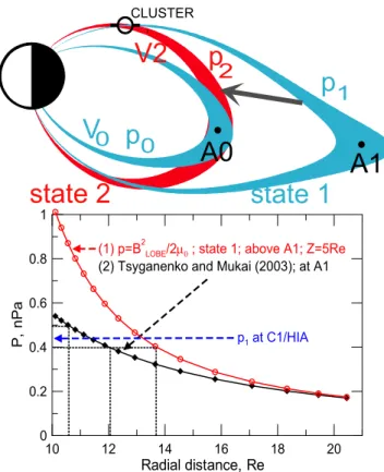
Still, the spacecraft coverage is far from optimum in this case, so we also tried another (relatively independent) method to specify the equatorial location and, most impor-tantly, to constrain the change between the initial state and the final stage (when the injection peak was observed at the Cluster location) of the localized injected plasma flux tube. As in some previous studies (Delcourt et al., 1992; Smets et al., 1999), we assume that the major flux tube geometry change is due to the dipolarization and contrac-tion (earthward mocontrac-tion) of its equatorial part (due to the change/redistribution of the tail currents and resulting in-ductive electric field), whereas the change in its ionospheric footpoint is insignificant, because the process is very short in duration. This situation, as schematically shown in Fig. 11, means that the initial (1) and final (2) flux tube locations are close to each other in the plasma sheet horns probed by Clus-ter, so that a comparison of the accelerated electron spectra in the peak of the event (state 2) with those observed just be-fore the event (state 1 in Fig. 11) can be used to characterize the amount of acceleration in the contracting plasma tube.

To realize this idea, we used the following scheme (see de-tails in Appendix). We used theKp-dependent T89 model by

introducing a non-integerK_p∗(the corresponding model field was computed by the linear interpolation between the field values in two neighboring integerKp models). We

com-pared the amount of electron acceleration in the adiabatic approximation between the two configurations (1 and 2 in Fig. 11, characterized by initialKp∗₁ and finalKp∗₂ values, respectively) of the field line passing through the location of Cluster-1 (see details in the Appendix). By doing this we specify the change in the properties of one particular flux tube rather than determine the entire magnetic configuration change. We tried differentKp∗

1 values in the range 0.5–1.5 (with 0.1 step), motivated by the previous observation that theKp=1 model fits best to the B-fields observed just prior

to the injection. For eachKp₁∗we varied theKp₂∗value (also with 0.1 step) to find the best match to the electron acceler-ation expected on the field line which is passed through the C1 location. The results are given in Table 1, the fit goodness measure,σ, in logarithmic scale, is also shown.

10 12 14 16 18 20

Radial distance, Re

0 0.2 0.4 0.6 0.8 1

P,

n

Pa

p1 at C1/HIA

(1) p=B2LOBE/2μ0 ; state 1; above A1; Z=5Re

(2) Tsyganenko and Mukai (2003); at A1

Fig. 11.Sketch explaining the dipolarization and entropy compar-isons (top). Cluster 1 pressure value before the injection compared with empirical pressure profile of plasma sheet ions by Tsyganenko

and Mukai (2003) and with magnetic pressure in lobes Z=5R_E

above A1 point (bottom).

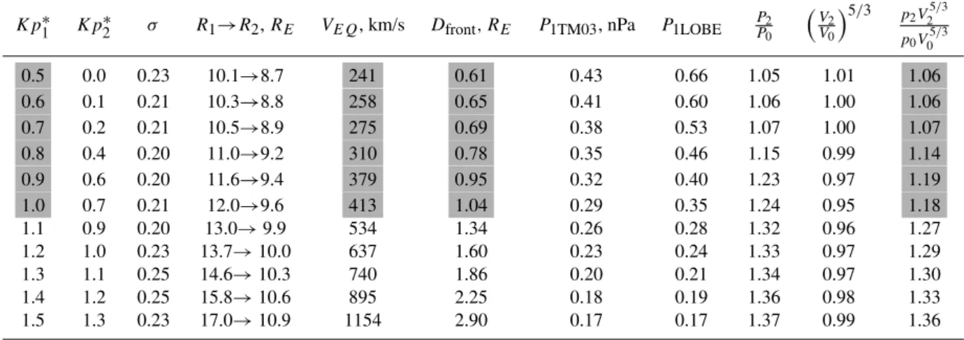
As seen from Table 1, the acceleration is reproduced with the smallest errors (σ=0.20–0.21) when the initial flux tube location was at 10–12RE distance range. We should also

note that the σ value is sensitive to the change between the flux tube states 1 and 2 more than to its initial location (state 1). To clarify and limit the initial equatorial location we use the observed plasma pressure as an additional filter. The pressure is computed in the equatorial section of flux tube 1 from the empirical plasma model by Tsyganenko and Mukai (2003),P1TM03. We comparedP1TM03 with the ob-servations to indicate if an initial state was realistic or not. The comparison in Fig. 11b indicates that the observed pres-sure (∼0.4 nPa at C1 and∼0.9 nPa C4 before the injection) could only be observed at distances 9–13RE. The possible

underestimation of the equatorial pressure measured by the CIS intrument (e.g. due to presence of heavy ions) favors the closer initial flux tube location. This eliminates the bottom part of Table 1 as unrealistic and allows one to identify the initial location to be at<11–13REradial distances.

Table 1. DifferentK_p∗pairs, standard deviation, injection front observed at C1 and C4 mapped to the equatorial plane, front propagation speed, front thickness, initial pressure obtained from Tsyganenko and Mukai (2003) and vertical pressure balance. The injected flux tube parameters (pressure, volume, entropy) related to those in the neigbouring flux tubes.

Kp₁∗ Kp₂∗ σ R1→R2,RE VEQ, km/s Dfront, RE P1TM03, nPa P1LOBE P_P2₀

_V

2

V0

5/3 _p

2V25/3

p0V05/3

0.5 0.0 0.23 10.1→8.7 241 0.61 0.43 0.66 1.05 1.01 1.06

0.6 0.1 0.21 10.3→8.8 258 0.65 0.41 0.60 1.06 1.00 1.06

0.7 0.2 0.21 10.5→8.9 275 0.69 0.38 0.53 1.07 1.00 1.07

0.8 0.4 0.20 11.0→9.2 310 0.78 0.35 0.46 1.15 0.99 1.14

0.9 0.6 0.20 11.6→9.4 379 0.95 0.32 0.40 1.23 0.97 1.19

1.0 0.7 0.21 12.0→9.6 413 1.04 0.29 0.35 1.24 0.95 1.18

1.1 0.9 0.20 13.0→9.9 534 1.34 0.26 0.28 1.32 0.96 1.27

1.2 1.0 0.23 13.7→10.0 637 1.60 0.23 0.24 1.33 0.97 1.29

1.3 1.1 0.25 14.6→10.3 740 1.86 0.20 0.21 1.34 0.97 1.30

1.4 1.2 0.25 15.8→10.6 895 2.25 0.18 0.19 1.36 0.98 1.33

1.5 1.3 0.23 17.0→10.9 1154 2.90 0.17 0.17 1.37 0.99 1.36

limit of our estimate. With the initial location of the injected plasma tube in the range of 11–13RE, the propagation speed

mapped to the equatorial region is 200–400 km/s, and the spatial scale of the frontside layer is about 1RE. The

dis-tance range of the flux tube contraction and velocities are comparable to those used in the EM pulse simulations by Li et al. (1998). They used 100 km/s velocity EM pulse, which was initiated at 40REto describe the observations at 6.6RE.

Having in mind the picture of an azimuthally localized in-jected plasma tube we may attempt to compare this flux tube (at final state 2) with the flux tube at the same distance but at a different longitude, outside the injection sector (flux tube 0 in Fig. 11). To do that we assume that the ambient plasma and magnetic configuration are not strongly affected during the localized injection (or that the injected flux tube has a small azimuthal extent). In this case we can use the state 1 model withKp∗₁ to specify the parameters of plasma flux tube 0 and state 2 model withKp∗₂to specify the parameters of the plasma tube 2. From these models we can easily compute the volumes of the unit magnetic flux tube (V=Rds/B) at these locations. Also, by assuming force equilibrium in the midnight equatorial plane (∇P=[j×B]), we may compute the plasma pressure at the point A0 from theKp₁∗model by integrating∇P along the tail axis from point A1 to the point A0 asP0=P1+R_AA₁0[j×B]dl. Here the pressureP1observed by Cluster before the injection is used as the initial value, whereas the cross tail current density (j) and magnetic field (BZ) in the neutral sheet are computed from the state 1 model

(see Kubyshkina et al. (2002) for method testing).

The results of computation (Table 1) show that in the equa-torial plane the pressure in the injected tube is comparable to that in the neigboring flux tubes (in MLT sense) (P2∼P0), inspite of the noticable pressure increase during the injection (P2≈1.5−1.7P1). The net change in the plasma tube entropy

parameterP V5/3_{is such that the entropy of the injected flux} tube is still comparable with the value in the ambient flux tubes,P2V₂5/3/P0V₀5/3∼1.0 at the final observation location. This implies that the injected plasma parcel may have had a property of a plasma bubble during the earlier stages of its evolution. This is consistent with the conclusions of the previous case and statistical studies of fast flow bursts in the magnetotail (e.g. Sergeev et al., 1996b; Sch¨odel et al., 2001; Nakamura et al., 2001b; Lyons et al., 2003).

5 Discussion

5.1 Summary of observations

Both energy-dispersed and dispersionless injections were ob-served at LANL and Cluster satellites near the midnight meridian. The similarity in the activity associated with the energy-dispersed and the dispersionless injections allows us to interpret them as similar objects and prescribe the different appearence to the different spacecraft locations with respect to the injection proper. We summarize our observations:

1) As compared to the dispersed injection “i1” which had no stable signatures in the magnetic and electric field the dis-persionless injection “i2” (observed at Cluster) had the fol-lowing distinctive properties repeated at all 4 spacecraft: (a) a simultaneous increase in the electron fluxes at all energies between 1 and 300 keV during∼16 s (“injection front”); (b) an increase in theBZ magnetic field component by∼30 nT

at the dipolarization front; (c) an increase in the plasma pres-sure by a factor of 1.5–1.7 at the dipolarization front; (d) a bipolar-like turbulent variation in the electric fieldEY

by all 4 satellites with appropriate time shift, these properties characterize the spatial structure associated with dispersion-less injections.

2) Four spacecraft allowed us to identify a sharp injec-tion/dipolarization front that propagated inward, with a prop-agation speed and front thickness estimated to be∼25 km/s (with some deceleration) and 400 km, respectively, at the ob-servation region in the plasma sheet horns, at 5REgeocentric

distance, where the magnetic field magnitude was 600 nT. After tuning the magnetic field model and mapping to the equatorial distance at R∼9–12RE, we obtain (see Sect. 4)

an earthward velocity of V∼200–400 km/s and a thickness of∼1REin the equatorial plane.

3) Based on IMAGE/WIC observations we attempted to identify auroral structures detected together with injections. The auroral oval was rather faint with poleward/equatorward boundaries at∼71.5/63◦_{from the DMSP F14 flyby at 03:25–} 03:29 UT. Two poleward boundary intensifications (marked by “S1” and “S2” in Fig. 4), propagating equatorward, had lifetimes of 4–6 min, as observed by IMAGE/WIC, and could possibly be associated with the injections observed by LANL and Cluster at perigee. “S1”, initiated at 03:18 UT, was pos-sibly related to injection “i1” at 03:19 UT, and “S2”, initiated at 03:22 UT, was possibly associated with the dispersionless injection “i2” at 03:27 UT.

4) Electron pitch angle distributions observed by PEACE (0.05–27 keV) showed two kinds of anisotropy, bi-directional at E<2 keV and pancake at E>5 keV. A sharp inner boundary of the bi-directional distributions (at 0.1– 3 keV) was found before (i.e. deeper inside the magneto-sphere) than the injection, mapping at a 8–10RE distance

in the equatorial plane. This boundary seemed to be spa-tially stable and was unrelated to the injection, and this will be a subject of a future study. The character of the electron anisotropy did not change while the particle flux increased during the injection front passage.

The properties of the dispersionless injection front con-firm that we observed a localized plasma structure passing the chain of Cluster spacecraft. Its localization in the az-imuthal direction is supported by narrow auroral structures and by the absense of magnetic pulse signatures at the G12, which was only 2 h in MLT away from the injection obser-vations. We clearly see that the pulse associated with the dispersionless injection was spatially localized in the radial direction: spacecraft C4 did not record any changes at the time when the peak of the structure had already passed over the C1 satellite, 900 km away (see Fig. 9). There were no global changes in the magnetic field, electric field, or plasma properties. When using the term “dipolarization” or “dipo-larization front”, we therefore mean azimuthally and radially localized reconfiguration or propagating structure.

5.2 On the origin of plasma injections

Plasma injections, observed fluxes and dis-persed/dispersionless character, are simulated using the EM pulse model (Li et al., 1998; Sarris et al., 2002; Zaharia et al., 2004). These simulations describe the observations at the geostationary orbit, 6.6RE, and deeper, requiring

an earthward propagating structure with several tens–few hundreds km/s velocity, and enhanced duskward electric and northward magnetic fields. In this paper we presented multipoint observation of the dispersionless injection at a larger radial distance of 8–13RE, where only a few injection

observations have been done previously. The observed injection properties, propagation velocity, and electric and magnetic fields mostly fit the EM pulse requrements. This supports the EM pulse idea, although it is not yet clear what generates such structures and transports them earthward (e.g. there is no MHD wave propagating with such a slow speed). We suppose bursty bulk flows (BBFs) propagating as a plasma structure (not a wave) to be responsible for the EM pulse transport and, thereby, the energetic particle origin. The observed dispersionless injection structure mapping at 8–13RE propagated ∼2RE earthward at a 200–400 km/s

speed. The similar velocities are known for rapid flux tranfer events (RFT) at this distance (∼200 km/s, on average, after Sch¨odel et al., 2001). So, BBFs satisfy (1) the velocity limits; (2) azimuthal extent limits, both required for the EM pulse model and observed for the injections; (3) enhancedBZand

enhancedEY (e.g. Sergeev et al., 1996b). BBFs, however,

are mostly studied at a 10–15REradial distance and are

dif-ficult to observe closer to Earth due to a velocity decrease (Sch¨odel et al., 2001) and, probably, an occurrence decrease. We also discussed the possible connection between the in-jections and auroral streamers that was recently investigated by Sergeev et al. (2005). Streamers, in turn, are known to be associated with BBFs (Sergeev et al., 1999, 2000; Nakamura et al., 2001a; Lyons et al., 2002).

Our detailed observations of the injection in the transition region (8–13RE) provide a link between the EM pulse

(con-sidered in the inner region) and BBFs (studied at>10RE)

previously discussed as separate phenomena. We suggest that fast narrow plasma streams (BBFs), which have the bub-ble property, are the very probabub-ble mechanism of plasma in-jections into the inner magnetosphere.

Appendix A

Modeling of adiabatic heating

100 1000 10000

Energy, eV

1x10

-5

1x10

-4

JE, differential energy flux

ergs/(cm^2 s sr eV)

Modeled

Final observed

Initial observed

100 1000 10000

Energy, eV

1x10

-5

1x10

-4

100 1000 10000

Energy, eV

1x10

-5

1x10

-4

100 1000 10000

Energy, eV

1x10

-5

1x10

-4

JE, differential energy flux

ergs/(cm^2 s sr eV)

100 1000 10000

Energy, eV

1x10

-5

1x10

-4

CLUSTER 1

Ininital

_{3 spin averaged 3:26:31-39 compared with}

final

_3:26:43-51

Field line fixed at SC location; transition from T89 Kp*=0.5 tp Kp*=0.0

PA=0-7.5

PA=7.5-22.5

PA=22.5-37.5

PA=37.5-52.5

PA=52.5-67.5

100 200 300 400

90 80 70 60 50 40 30

Energy, keV

1.0x10

3

1.0x10

4

1.0x10

5

1.0x10

6

J

E

, d

iffe

re

n

ti

a

l e

n

e

rg

y

fl

u

x

ke

V

/(

cm

^

2

s sr

ke

V

)

RAPID

we suppose it measures only 45-90 deg

Modeled

Observed final

Observed initial

RAPID

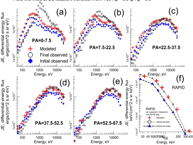
Fig. A1. Comparison of electron spectra observed before (blue diamonds) and after (black circles) the injection with the modeled spectra (red pluses). Panels(a–e)correspond to different pitch angles at PEACE, higher energy spectra part from RAPID is at panel(f).

(1999). We assume conservation of the first two adiabatic invariants for electrons, as well as phase space density (Li-ouville theorem).

As input data we use Cluster/PEACE observations from 30 energy channels in the range 0.036–24 keV for electrons with a 15-degree pitch angle resolution. Taking every energy and every pitch angle bin and using observed initial (before the injection) differential energy fluxJE(W1, αCL)we do the

following:

(1) Transform the pitch angle from the Cluster location to the equatorial plane using the magnetic configuration in state 1 to obtainJE(W1, αEQ)(in-situ pitch angles are mapped to

the equatorial ones using sin2αEQ=sin2αCL·BEQ/BCL);

(2) Calculate the increase in the perpendicular energy component due to betatron acceleration (from conservation of the magnetic moment) asWperp2=Wperp1∗Beq2/Beq1;

(3) Calculate the increase of the parallel energy com-ponent using the second adiabatic invariant conservation,

Wpar2=Wpar1∗FL2₁/FL2₂, where FL1 and FL2 are the field line lengths between the mirror points in states 1 and 2. Since the mirror point locations (FL1, FL2 as well) depend on the particle pitch angles, an iterative search is required. Pre-scribing minimum and maximum Wpar values (which corre-spond to minimum and maximum of the longitudinal invari-antJ2=Wpar2·FL2₂as well), we use the dichotomy algorithm to satisfy J2 approaching J1 to an accuracy less than 0.1%;

(4) Using the Liouville theorem

(f (W, a)=JE/W2=const) we obtain the new energy

flux valueJE(W2, a2);

In the case of Cluster observations we distribute the mod-eled fluxes among the bins for energies and pitch angles used by the Cluster/PEACE instrument. Choosing the initialKp∗

1, and taking the spectrum before the injection,J_E1(W, α), we compute the model fluxJ_Emodel(W, α)using the scheme de-scribed above. By varying the finalKp₂∗models we looked for the model that provided the best fit between modeled fluxes and those observed at the injection peak, J_E2(W, α). We use logarithmic standard deviation between the observed flux and the modeled flux,σ=P

log(J_Emodel/J_E1)

, summed

over energies and pitch angles. Only bins with E>5 keV are used, because the presence of a field-aligned potential drop may cause serious distorsions for low-energy and low-pitch-angle particles (see Fig. A1a). The results of the comparison for the best fit are shown in Fig. A1. Calculated standard de-viations for the resultingK_p∗ pairs are presented in Table 1. Theσ values are in the range 0.20–0.25 when including the contribution from low pitch angles (<7.5◦); for larger pitch angles only the standard deviation is much smaller,σ≈0.1. For comparison, the difference between the observed initial and observed accelerated distributions,σ=P

log(J_E2/J_E1) ,

is 0.45.

Acknowledgements. The preliminary AE index data were made available at Kyoto WDC-C data base. The electric field data are thanks to Cluster EFW instrument (M. Andre, PI). DMSP data was produced JHU/APL. ACE spacecraft data provided by N. Ness (Bartol Research Institute). The midlatitude magnetometer data was provided by INTERMAGNET. The work by S. V. Apatenkov was supported by INTAS-05-109-4496 grant. The research was also supported by INTAS 03-51-3738 grant and president grant for Leading Scientific Schools 8667.2006.5. S. V. Apatenkov and V. A. Sergeev thank the Austrian Academy of Sciences for the sup-port during their stay in Graz.

Topical Editor I. A. Daglis thanks two referees for their help in evaluating this paper.

References

Arnoldy, R. L. and Chan, K. W.: Particle substorm observed at the geostationary orbit, J. Geophys. Res., 74, 5019–5028, 1969. Baker, D. N., Higbie, P. R., Hones, E. W., and Belian, R. D.:

High-resolution energetic particle measurements at 6.6RE 3. Low-energy electron anisotropies and short-term sustorm predictions, J. Geophys. Res., 83(A10), 4863, 1978.

Balogh, A., Carr, C. M., Acuna, M. H., et al.: The Cluster magnetic field investigations: overview of in-flight performance and initial results, Ann. Geophys., 19, 1207–1217, 2001,

http://www.ann-geophys.net/19/1207/2001/.

Belian, R. D., Gisler, G. R., Cayton, T., and Christensen, R.: High-Z energetic particles at geosynchronous orbit during the great solar proton event series of October 1989, J. Geophys. Res., 97(A11), 16 897–16 906, doi:10.1029/92JA01139, 1992.

Birn, J., Raeder, J., Wang, Y. L., Wolf, R. A., and Hesse, M.: On the propagation of bubbles in the geomagnetic tail, Ann. Geophys., 22, 1773–1786, 2004,

http://www.ann-geophys.net/22/1773/2004/.

Delcourt, D. C. and Moore, T. E.: Precipitation of Ions Induced by Magnetotail Collapse, J. Geophys. Res., 97(A5), 6405–6415, doi:10.1029/91JA03142, 1992.

Gustafson, G., Andre, M., Carozzi, T., et al.: First results of electric field and density observations by Cluster EFW based on initial months of operation, Ann. Geophys., 19, 1219–1240, 2001, http://www.ann-geophys.net/19/1219/2001/.

Johnstone, A. D., Alsop, C., Burge, S., et al.: Peace: a Plasma Electron and Current Experiment, Space Sci. Rev., 79, 351–398, 1997.

Kubyshkina, M. V., Sergeev, V. A., and Pulkkinen, T.

I.: Hybrid Input Algorithm: An event-oriented

magneto-spheric model, J. Geophys. Res., 104(A11), 24 977–24 994, doi:10.1029/1999JA900222, 1999.

Kubyshkina, M. V., Sergeev, V. A., Dubyagin, S. V., Wing, S., Newell, P. T., Baumjohann, W., and Lui, A. T. Y.: Construct-ing the magnetospheric model includConstruct-ing pressure measurements, J. Geophys. Res., N6, 1070, doi:10.1029/2001JA900167, 2002. Li, X., Baker, D. N., Temerin, M., Reeves, G. D., and Belian, R. D.:

Simulation of dispersionless injections and drift echoes of ener-getic electrons associated with substorms, Geophys. Res. Lett., 25(20), 3763–3766, doi:10.1029/1998GL900001, 1998. Li, X., Sarris, T. E., Baker, D. N., and Peterson, W. K.:

Sim-ulation of energetic particle injections associated with a sub-storm on August 27, 2001, Geophys. Res. Lett., 30(N1), 1004, doi:10.1029/2002GL015967, 2003.

Lyons L. R., Zesta, E., Xu, Y., Sanchez, E. R., Samson, J. C., Reeves, G. D., Ruohoniemi, J. M., and Sigwarth, J. B.: Auro-ral poleward boundary intensifications and tail bursty flows: A manifestation of a large-scale ULF oscillation?, J. Geophys. Res., 107(A11), 1352, doi:10.1029/2001JA000242, 2002.

Lyons, L. R., Wang, C.-P., Nagai, T., Mukai, T., Saito, Y., and Samson, J. C.: Substorm inner plasma sheet particle reduction, J. Geophys. Res., 108(A12), 1426, doi:10.1029/2003JA010177, 2003.

Moore, T. E., Arnoldy, R. L., Feynman, J., and Hardy, D. A.: Prop-agating substorm injection fronts, J. Geophys. Res., 86, 6713– 6726, 1981.

Nakamura, R., Baumjohann, W., Brittnacher, M., Sergeev, V. A., Kubyshkina, M., Mukai, T., and Liou, K.: Flow bursts and auro-ral activations: Onset timing and foot point location, J. Geophys. Res., 106(A6), 10 777–10 790, doi:10.1029/2000JA000249, 2001a.

Nakamura, R., Baumjohann, W., Sch¨odel, R., Brittnacher, M.,

Sergeev, V. A., Kubyshkina, M., and Mukai, T., and

Liou, K.: Earthward flow bursts, auroral streamers, and

small expansions, J. Geophys. Res., 106(A6), 10 791–10 802, doi:10.1029/2000JA000306, 2001b.

Ohtani, S.-I.: Earthward expansion of tail current disruption: Dual-satellite study, J. Geophys. Res., 103, 6815–6825, 1998. Reeves, G. D., Belian, R. D., and Fritz, T. A.: Numerical tracing of

energetic particle drifts in a model magnetosphere, J. Geophys. Res., 96(A8), 13 997–14 008, doi:10.1029/91JA01161, 1991. Reeves, G. D., Henderson, M. G., McLachlan, P. S., Belian, R. D.,

the identical Cluster ion spectrometry (CIS) experiment, Ann. Geophys., 19, 1303–1354, 2001,

http://www.ann-geophys.net/19/1303/2001/.

Sarris, T. E., Li, X., Tsaggas, N., and Paschalidis, N.: Mod-eling energetic particle injections in dynamic pulse fields with varying propagation speeds, J. Geophys. Res., 107(A3), doi:10.1029/2001JA900166, 2002.

Sch¨odel, R., Nakamura, R., Baumjohann, W., and Mukai, T.: Rapid flux transport and plasma sheet reconfiguration, J. Geophys. Res., 106, 8381–8390, 2001.

Sergeev, V. A., Vagina, L. I., Elphinstone, R. D., Murphree, J. S., Hearn, D. J., Cogger, L. L., and Johnson, M. L.: Comparison of UV optical signatures with the Substorm Current Wedge pre-dicted by an inversion algorithm, J. Geophys. Res., 101(A2), 2615–2628, doi:10.1029/95JA00537, 1996a.

Sergeev, V. A., Angelopoulos, V., Gosling, J. T., Cattell, C. A., and Russell, C. T.: Detection of localized, plasma-depleted flux tubes or bubbles in the midtail plasma sheet, J. Geophys. Res., 101(A5), 10 817–10 826, doi:10.1029/96JA00460, 1996. Sergeev, V. A., Shukhtina, M. A., Rasinkangas, R., Korth,

A., Reeves, G. D., Singer, H. J., Thomsen, M. F., and Vagina, L. I.: Event study of deep energetic particle injec-tions during substorm, J. Geophys. Res., 103(A5), 9217–9234, doi:10.1029/97JA03686, 1998.

Sergeev, V. A., Liou, K., Meng, C.-I., Newell, P. T., Brit-tnacher, M., Parks, G., and Reeves, G. D.: Development of au-roral streamers in association with localized impulsive injections to the inner magnetotail, Geophys. Res. Lett., 26(3), 417–420, doi:10.1029/1998GL900311, 1999.

Sergeev, V. A., Sauvaud, J.-A., Popescu, D., Kovrazhkin, R. A., Liou, K., Newell, P. T., Brittnacher, M., Parks, G., Nakamura, R., Mukai, T., and Reeves, G. D.: Multiple-spacecraft observation of a narrow transient plasma jet in the Earths plasma sheet, Geo-phys. Res. Lett., 27(6), 851–854, doi:10.1029/1999GL010729, 2000.

Sergeev, V. A., Yahnin, D. A., Liou, K., Thomsen, M. F., and Reeves, G. D.: Narrow Plasma Streams as a candidate to pop-ulate the inner magnetosphere, Geophys. Monogr. Ser., p. 155, 2005.

Smets, R., Delcourt, D., Sauvaud, J. A., and Koperski, P.: Electron pitch angle distributions following the dipolarization phase of a substorm: Interball-Tail observations and modeling, J. Geophys. Res., 104(A7), 14 571–14 576, doi:10.1029/1998JA900162, 1999.

Thomsen, M. F., Birn, J., Borovsky, J. E., Morzinski, K., McComas, D. J., and Reeves, G. D.: Two-satellite observations of substorm injections at geosynchronous orbit, J. Geophys. Res., 106(A5), 8405–8416, doi:10.1029/2000JA000080, 2001.

Tsyganenko, N. A.: A magnetospheric magnetic field with a warped tail current sheet, Planet. Space Sci., 37, 5–20, 1989.

Tsyganenko, N. A.: Modeling the Earth’s magnetospheric magnetic field confined within a realistic magnetopause, J. Geophys. Res., 100, 5599–5612, 1995.

Tsyganenko, N. A. and Mukai, T.: Tail plasma sheet models derived from Geotail particle data, J. Geophys. Res., 108(A3), 1136, doi:10.1029/2002JA009707, 2003.

Wilken, B., Daly, P. W., Mall, U., et al.: First results from the RAPID imaging energetic particle spectrometer on board Clus-ter, Ann. Geophys., 19, 1355–1366, 2001,

http://www.ann-geophys.net/19/1355/2001/.