Some Results on the Experimental Implementation
of a State-Affine Observer for a DC Motor
R. Salas-Cabrera, J. G. Gonzalez-Hernandez, J. de-Leon-Morales, J. C. Rosas-Caro, A. Gonzalez-Rodriguez,
E. N. Salas-Cabrera and R. Castillo-Gutierrez
Abstract—This work deals with the experimental results of implementing a nonlinear state-affine observer for a shunt connected DC motor. The observer is able to estimate the state variables and one unknown parameter. The rest of the parameters are modeled by algebraic functions that are based on data obtained from experimental steady state and transient tests. Estimated states are compared to the corresponding experimental states. A free open source Linux distribution and a commercial data acquisition board are used as the real-time platform.
Index Terms—state-affine observer, DC motor, data acquisi-tion, real-time.
I. INTRODUCTION
S
TATE observers are based on a dynamic model that usually supposes the exact knowledge of all of the parameters. If parameters vary, then the accuracy of the state estimation diminishes. Since an improved version of the state variables and parameters may provide a more reliable closed loop performance, it is desirable to address the estimation of most of the state variables and the dynamic identification of most of the parameters. On the other hand, it is well known that parameters of any electric machine depend on the operating conditions. In practice, they depend on steady state and even transient conditions. Therefore, variations of parameters are expected to occur during any experimental test. In this work we represent the parametric variations by defining algebraic functions depending on some of the state variables. These algebraic descriptions are derived by using the off-linedata that are obtained from experimental steady state and transient tests.Our aim is to estimate some state variables and to identify the load torque by using the nonlinear state affine observer, whereas the rest of the parameters are represented by the mentioned algebraic descriptions. Similarly, contribution [1] proposes several nonlinear observers for estimating the state and the load torque. In contrast, the interesting contribution in [1] refers to a series-connected DC motor where most of the parameters are assumed to be constant.
Manuscript received July 11, 2011; revised August 10, 2011. This work was supported by DGEST under grants No. 360710P ”Sintesis e implementacion de un emulador de un aerogenerador en tiempo real” and No. 360810P ”Analisis de topologias de convertidores de potencia con capacidad de flujo de potencia bidireccional”.
R. Salas-Cabrera, A. Gonzalez-Rodriguez, E.N. Salas-Cabrera, R. Castillo-Gutierrez and J.C. Rosas-Caro are with the Instituto Tecnologico de Ciudad Madero, Departamento de Ingenieria Electrica y Electronica, Division de Estudios de Posgrado e Investigacion, Cd. Madero, Mexico (email: [email protected];[email protected]).
J. de Leon Morales is with the Universidad Autonoma de Nuevo Leon, Facultad de Ingenieria Mecanica y Electrica, San Nicolas de los Garza, Mexico.
J.G. Gonzalez-Hernandez is with the Universidad Tecnologica de Al-tamira, Departamento de Mecatronica, AlAl-tamira, Mexico.
In our work, a ninth-order dynamic system that includes some state equations for the dynamic gains is solved by the real-time platform. The subsystem to be observed is a third order nonlinear dynamic system.
Some mathematical tools may be used to perform state estimation and parametric identification simultaneously, see [2] [3] [4] [5]. Several reduced order nonlinear observers have been proposed in the literature for sensorless appli-cations, [6]. There are some previous works related to the observation problem of MIMO state affine systems with constant unknown parameters [7]. There are other works that deal with state estimation for affine linear parameter varying systems [8]. In contrast, our investigation addresses parametric variations that are non-linear.
In this work, we employ RTAI-Lab [9]. It is a free open-source Linux-based real-time software. It has been used in previous works, [1], [10], [11], [12]. Contribution [10] describes an RTAI-Lab application for a DC motor where a discrete-time linear time-invariant observer is implemented. Contributions [1], [10] and [11] consider that all of the parameters associated to the electric subsystem of the motor are constant. In contrast, we employ a nonlinear state-affine observer with non-constant parameters. Improved results are presented in this paper since it involves the natural nonlinear behavior associated to this type of systems and considers the parametric variations.
II. MODELING OF THEDCMACHINE
A. State Space Representation
Consider the following nonlinear dynamic equation that describes the transient and steady state behavior of a shunt connected DC motor
d dt
ia
wr
if
=
−raia
Laa −
kaΦwr
Laa +
va
Laa
kaΦia
J −
TL
J
−rfif
Lf f +
va
Lf f
y=[ iaif]
T
(1)
where x = [ia wr if]T is the state, u = va is the input,
y= [iaif]T is the measured output,Φ is the direct-axis air gap flux and ka is a constant defined by the design of the winding. Standard notation is employed for the rest of the variables/parameters.
B. Parametric identification
was recorded. Figure 1 shows several experimental transient traces for different step voltages. An off-line calculation is then performed to obtain the field inductance. The armature inductance was obtained by carrying out similar experimental tests. Both armature and field resistances were calculated after obtaining experimental data from several steady state tests.
0 0.05 0.1 0.15 0.2 0.25 0.3
0 0.02 0.04 0.06 0.08 0.1 0.12
Time(s)
If(A)
Fig. 1. Experimental traces of the field current
All of those tests have suggested that different mathemat-ical functions are necessary for an adequate representation of the parameters. In practice, each one of the parameters depend on a particular state variable that is associated to the actual operating conditions. As an example, Figure 2 shows the self-inductance of the field winding as a function of the field current. It depicts both the experimental data and the corresponding data obtained by using a function-based representation.
−0.48 −0.2 0 0.2 0.4
10 12 14 16 18 20 22 24
if(amp.)
Lff (H)
Fig. 2. Lf f, (*) experimental data, (-) function-based data.
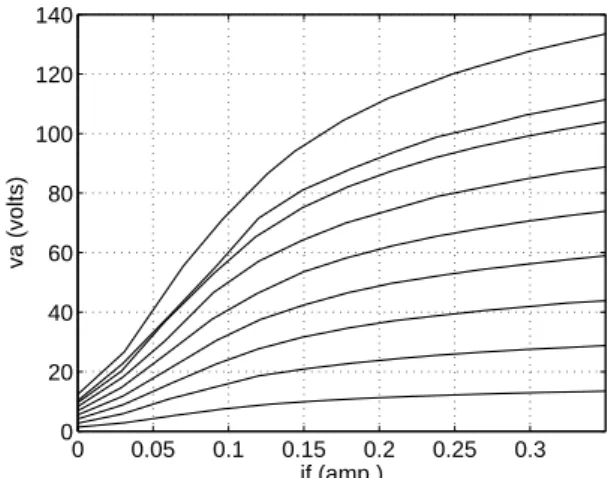
The direct-axis air gap flux, denoted by Φ, is in general associated to the field currentif. A standard assumption for the ideal DC machine is that magnetic saturation is neglected. In other words,kaΦ =LAFif. In our case, the experimental data presented in Figure 3 define a nonlinear relationship between the open circuit armature voltage va and if or equivalently between kaΦandLAFif.
Even more, using the experimental data shown in Figure 3 and the first expression of the state equation in (1) the
0 0.05 0.1 0.15 0.2 0.25 0.3
0 20 40 60 80 100 120 140
if (amp.)
va (volts)
Fig. 3. Experimental magnetization curves for different rotor speeds.
kaΦ-if relationship is obtained, see Figure 4.
0 0.1 0.2 0.3 0.4
0 0.2 0.4 0.6 0.8
if (amp.)
ka Phi (volt−sec/rad)
Fig. 4. kaΦ-if . (*) experimental data, (-) function-based data.
Considering all of the experimental data obtained from several transient and steady state tests adequate expressions for the each one of the parameters are proposed:
Lf f =A1+A2 √
|if |; Laa=B1+B2 √
|ia|
kaΦ =C1+C2 √
|if |; rf =D1i2f+D2if+D3 ra=E1i2a+E2ia+E3
(2)
It is important to note that the expression forkaΦincludes the voltage associated to the residual flux that is evident from the experimental magnetization curves, see Figure 3 . Stan-dard procedures for curve fitting are employed for calculating each constant involved in the above representations, i.e.
[A1A2] =[9.125 22.495]
[B1B2] =[5.323x10⁻³ 22.972x10⁻³]
[C1C2] =[0.0099 1.2215]
[D1D2D3] =[262.60 0 324.6772]
[E1E2E3] =[0.0788 0 7.5815]
(3)
N.m. In contrast, the load torque TL is considered as an unknown time-varying parameter to be estimated. Custom-made electronics designs are employed for the observer im-plementation and theoff-lineidentification of the parameters.
III. ANALYSIS OF OBSERVABILITY
In this section the analysis of the observability is carried out. From (1) we can write the following dynamic subsystem
˙
z = f(z, ym) +ϕ(u, ym)
h = ym (4)
where
f(z, ym) =
f1 f2 f3 =
−raia
Laa −
kaΦwr
Laa
kaΦia
J − TL J 0
ϕ(u, ym) =
va Laa 0 0 ; z=
ia wr TL
h=ym=ia; u=va The space of functions O is given by
O = {h, Lfh(z), L2fh(z)}
= {ia, −
raia
Laa
−kaΦωr
Laa
, L2fh(z)}
where
Lfh(z) =f1
and
L2fh(z) =
∂f1 ∂ia
f1− kaΦωr
LaaJ
TL=F2
Then, the observation space is given by
dO=
dh dLfh(z)
dL2fh(z)
=
1 0 0
∂F2
∂ia −
kaΦ
Laa 0
0 0 −kaΦωr
LaaJ
Calculating the determinant ofdO, we obtain
det{dO}= k
2
aΦ2
J L2
aa
ωr
Ifdet{dO}is different to zero, then the system is observable. In other words, the system (4) is not observable if
ωr= 0 or
−k
2
aΦ2
J L2
aa
= 0
IV. OBSERVER FOR A STATE AFFINE SYSTEM
Consider the state affine system defined by
˙
z = A(ym)z+ϕ(u, ym)
ym = Cz (5)
where entries of the matrix A(ym)and the vectorϕ(u, ym) are uniformly bounded continuous functions depending onu
and/or ym, [4] [5]. Then, the system
˙ˆ
z = A(ym)ˆz+ϕ(u, ym) +Sz−1CTΣ(ym−Czˆ)
˙
Sz = −ρzSz−A(ym)TSz−SzA(ym) +CTΣC (6)
is an observer for (5). WhereSz(0)>0,ρz is a sufficiently large positive constant andΣ is a bounded positive definite matrix. Moreover, the estimation error (ez := ˆz−z) con-verges exponentially to zero with a rate that is defined by
ρz. A detailed proof of the stability of the estimation error can be found in [5].
From (1) we can write the following dynamic subsystem
d dt ia wr TL =
0 −kaΦ
Laa 0
0 0 −1
J
0 0 0
ia wr TL +
−raia
Laa +
va
Laa
kaΦia
J
0
ym = Cz=[1 0 0] [ia wr TL] T
(7)
By comparing the above equation and the dynamic system in (5), it is clear the definition forz,A(u, ym),ϕ(u, ym)and
C. Parameters are defined by expressions given by (2). After a long algebraic procedure and employing equations (6) and (7), the following ninth order state equation is obtained
˙ˆ ia ˙ˆ wr ˙ˆ TL ˙ˆ S11 ˙ˆ S12 ˙ˆ S13 ˙ˆ S22 ˙ˆ S23 ˙ˆ S33 =
(kaΦ ˆwr−raia+Va)
Laa −
(S22S33−S23 2
)(ia−ˆia)
|Sz| ˆ
TL+kaΦia
J +
(S23S13−S12S33)(ia−ˆia)
|Sz| (S12S23−S22S13)(ia−ˆia)
|Sz|
−ρzS11+ 1
−ρzS11+kaLΦaaS11
−ρzS13+SJ12
−ρzS22+2kaLΦaaS12
−ρzS23+kaLΦaaS13 +SJ22
−ρzS33+2SJ23
(8)
Expression defined by (8) will be used for implementing the nonlinear state-affine observer. It is clear that some of the variables/parameters involved in (8) are calculated by the real-time software while other variables are measured by the adquisition-board/real-time-software combination.
V. RESULTS
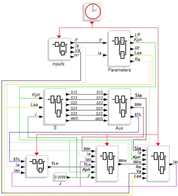
This section presents the experimental traces that result of applying the nonlinear state-affine observer to the DC motor. Expression (8) is solved by the real-time software (RTAI). The block-based main program is illustrated in Figure 5. In order to organize the block-based program several subroutines (superblocks) are included. As it is shown in Figure 5, three variables (if, ia and va ) have to be measured for solving the ninth order nonlinear state-affine observer. Several FIFO blocks are also used for recording the transient variables during the experiments. Details of the procedure for compiling the block-based program can be found in [1], [9] and [10].
Fig. 5. Main Scicos/Scilab program.
the initial 0.25 seconds. It shows the capabilities of the non-linear observer to reach the measured output. It is important to recall that the measured armature current is utilized to calculate the corrective term of the nonlinear observer. The first armature current peak in Figure 7 corresponds to the electromagnetic torque that is required to overcome the mechanical rotor inertia and the machine friction/losses during the start up. The rest of the current peaks in Figure 7 are due to the application of several random load torque steps at the shaft of the electric machine. From Figures 6 and 7 it is evident that once the observer-based variable reaches the measured variable, their behavior are identical even during the load torque disturbances. The electric machine is shut down at approximately 16 seconds. In this partic-ular test, the experimental system has the following initial conditions: [
ia(0) ωr(0) if(0)] T
= [
0 0 0]T
. The experimental initial conditions for the state affine observer
0 0.05 0.1 0.15 0.2 0.25
−1.5 −1 −0.5 0 0.5 1 1.5 2
Time(s)
Ia(A)
Observer−based
Measured
Fig. 6. Armature current.
are zˆ(0) = [ˆ
ia(0) ωˆr(0) TˆL(0)
]T
= [
2 10 1]T
;
Sz(0) =diag[1 1 1];ρz = 77;Σ = 1; andJ = 0.0058.
0 5 10 15 20
−2 −1 0 1 2 3
Time(s)
Ia(A)
Fig. 7. Armature current. (-) observer-based, (-) measured.
Figures 8 and 9 present the transient behavior of the rotor speed. Figure 8 corresponds to the initial 0.25 seconds of the experiment. It is clear that eventually, the observer-based state variable is very similar to the measured variable. Figure 9 shows the speed variations due to the start-up and the random application of the load torque. The experiment shows that the dynamic system in (7) holds the observability prop-erty even during non-power-up conditions. The experimental rotor speed is not strictly equal to zero due to the typical noise that appears normally during experimental tests (see Figure 8). As a consequence, the system (7) is observable. It is important to note that the non-linear observer is able to provide a reliable motor speed even during the random application of the load torque.
0 0.05 0.1 0.15 0.2 0.25
−10 −5 0 5 10 15
Time(s)
Wr (rad/s)
Observer−based
Measured
Fig. 8. Rotor speed.
The load torque is a parameter that is estimated by the non-linear observer. Figure 10 shows the transient behavior of the load torque. As it is expected, the peaks of the observer-based load torque illustrated in Figure 10 correspond to the rotor speed variations in Figure 9.
0 5 10 15 20 −20
0 20 40 60 80
Time(s)
Wr (rad/s)
Measured
Observer−based
Fig. 9. Rotor speed.
0 5 10 15 20 −0.5
0 0.5 1 1.5
Time(s)
TL(Nm)
Fig. 10. Observer-based load torque
nonlinear observer is required to work during an initial non steady state operation of the electric machine. These are more demanding conditions compared to the conditions of the previous test where the observer started to work during a steady state condition of the machine. Similar to the first test, several random load torque steps are applied to the shaft of the electric machine. The electric machine is shut down at 15.5 seconds approximately.
0 0.1 0.2 0.3 0.4 0.5
−20 −15 −10 −5 0 5 10
Time(s)
Ia(A)
Measured
Observed−based
Fig. 11. Armature current.
0 5 10 15 20 −20
−15 −10 −5 0 5 10
Time(s)
Ia(A)
Fig. 12. Armature current. (-) observer-based, (-) measured.
Figures 11 and 12 illustrate the dynamics of the measured armature current and its corresponding observed based version. Figure 11 presents the transient behavior during the initial 0.5 seconds. It is interesting to note how the value provided by the non-linear observer reaches the measured version of the armature current at 0.22 seconds approximately. Due to the simultaneous start up of the observer and the electric machine, increased estimated values are obtained, e.g. the observed based armature current is in the range of -20 to 7 amperes.
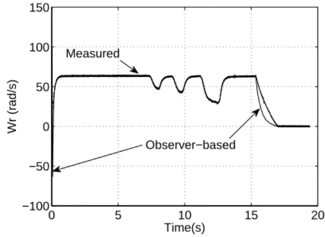
Figures 13 and 14 show the dynamics of the rotor speed. Figure 13 illustrates the initial 0.5 seconds. Increased val-ues are obtained due to the simultaneous start up of the observer and the electric machine. The nonlinear observer even reached negative rotor speeds. At approximately 0.22 seconds both the observer estimation and the measured rotor speed have almost the same values.
0 0.1 0.2 0.3 0.4 0.5
−100 −50 0 50 100 150
Time(s)
Wr (rad/s)
Observer−based Measured
Fig. 13. Rotor speed.
Figure 15 shows the transient behavior of the estimated load torque during this second test. The load torque provided by the observer reaches 12 Nm during the start up; this is about 10 times the peak value estimated during the first test. As it is expected, eventually the range of the estimated transient value for the load torque was similar to that obtained during the first experiment.
0 5 10 15 20 −100
−50 0 50 100 150
Time(s)
Wr (rad/s)
Observer−based Measured
Fig. 14. Rotor speed.
it is evident that those variations correspond to the rotor speed and armature current variations in Figure 12 and Figure 14 respectively.
0 5 10 15 20 0
2 4 6 8 10 12
Time(s)
TL(Nm)
Fig. 15. Observer-based load torque
VI. CONCLUSIONS
This work presents the experimental results of implement-ing a state-affine observer for a shunt connected DC motor. It considers the nonlinear dynamic nature associated to the electric machine and also involves the parametric variations. As a result, improved experimental transients have been obtained compared to those transients presented in previous works (see [1], [10], [11]).
REFERENCES
[1] N. Boizot, E. Busvelle, and J. Sachau. High-gain observers and Kalman filtering in hard real-time. RTL 9th Workshop, 2007.
[2] M. Ghanes, G. Zheng and J. De-Leon-Morales, On simultaneous parameter identification and state estimation for cascade state affine systems. Proc. of the American Control Conference, Seattle, WA, USA. 2008. pp. 45-50.
[3] Zhang Q., Adaptive observers for MIMO linear time-varying systems, IEEE Trans. on Automatic Control, Vol. 47, 2002, pp.525–529. [4] Besanc¸on G. and J. De-Le´on-Morales and O. Huerta, On
Adap-tive Observers for State Affine Systems, Internal Report-Laboratoire d’Automatique de Grenoble, France, 2005.
[5] Hammouri H. and J. De-Le´on-Morales , Observers synthesis for state affine systems, Proc. of the 29th IEEE Conf. Dec. and Control, Honolulu, Hawaii, 1990, pp. 784–785.
[6] Kumar R., Singh N. and Padmanaban S.V., A Nonlinear Reduced Order Observer for Rotor Position Estimation of Sensorless Permanent Magnet Brushless DC Motor Drive, IEEE Industrial Electronics, IECON 2006 32nd annual Conference, 2006. pp. 235-240
[7] Ahmed-Ali T., Postoyan R. and Lamnabhi Lagarrigue F., Continuos-discrete adaptive observers for state affine systems, Decision and Control, 46th IEEE Conference 2007. pp. 1356-1360
[8] Bara G.I., Dafouz J., Ragot J. and Kratz F., State estimation for affine LPV systems, Decision ans Control, Proc. of the 39th IEEE Conference, 2000. pp. 4565-4570 Vol. 5.
[9] R. Bucher, S. Mannori and T. Netter. RTAI-Lab tutorial: Scilab, Comedi and real-time control. 2008.
[10] R. Cabrera, J.C. Mayo-Maldonado, E.Y. Rendon-Fraga, E. Salas-Cabrera and A. Gonzalez-Rodriguez, On the experimental control of a separately excited DC motor, Lecture Notes in Electrical Engineering, Vol. 60, Springer, 2010.
[11] R. Salas-Cabrera, J. de-Leon-Morales, J.C. Mayo-Maldonado, J.C. Rosas-Caro, E.N. Salas-Cabrera, J.C. Reyna-Lopez, Observer design of DC Electric Machines, 2009 Second International Conference on Computer and Electrical Engineering, Dubai, United Arab Emirates. December 28 - 30, 2009.