doi:10.5194/nhess-12-1561-2012
© Author(s) 2012. CC Attribution 3.0 License.
and Earth
System Sciences
Drought analysis and short-term forecast in the Aison River
Basin (Greece)
S. Kavalieratou, D. K. Karpouzos, and C. Babajimopoulos
Dept. of Hydraulics, Soil Science and Agricultural Engineering, Faculty of Agriculture, Aristotle University of Thessaloniki, Greece
Correspondence to:C. Babajimopoulos ([email protected])
Received: 29 March 2011 – Revised: 28 January 2012 – Accepted: 7 February 2012 – Published: 21 May 2012
Abstract. A combined regional drought analysis and fore-cast is elaborated and applied to the Aison River Basin (Greece). The historical frequency, duration and severity were estimated using the standardized precipitation index (SPI) computed on variable time scales, while short-term drought forecast was investigated by means of 3-D loglin-ear models. A quasi-association model with homogenous diagonal effect was proposed to fit the observed frequen-cies of class transitions of the SPI values computed on the 12-month time scale. Then, an adapted submodel was se-lected for each data set through the backward elimination method. The analysis and forecast of the drought class tran-sition probabilities were based on the odds of the expected frequencies, estimated by these submodels, and the respec-tive confidence intervals of these odds. The parsimonious forecast models fitted adequately the observed data. Results gave a comprehensive insight on drought behavior, highlight-ing a dominant drought period (1988–1991) with extreme drought events and revealing, in most cases, smooth drought class transitions. The proposed approach can be an efficient tool in regional water resources management and short-term drought warning, especially in irrigated districts.
1 Introduction
Drought is an extreme recurrent climatic event characterized by lower than normal precipitation. Although it occurs in all climatic zones, its characteristics vary significantly from one region to another. Drought conditions can have critical envi-ronmental and economical impacts, especially in high water demanding areas with intensive agricultural activity. Various definitions of drought have been used, reflecting differences in regions, needs, and disciplinary approaches. Dracup et al. (1980) associate drought with precipitation (meteorolog-ical), streamflow (hydrolog(meteorolog-ical), soil moisture (agricultural)
or any combination of these parameters. A more extended classification is provided by Wilhite and Glantz (1985), where four approaches are proposed: meteorological, hy-drological, agricultural and socio-economic. The first three approaches deal with techniques to measure drought as a physical phenomenon, while the last one relates drought and socio-economic impacts that occured when demand for eco-nomic goods exceeds supply, as a result of a weather-related shortfall in water (Mishra and Singh, 2010).
Fig. 1.Aison River Basin – Pieria (Greece).
As drought management is increasingly adopting a risk-based approach (Sene, 2010), many countries are implement-ing drought monitorimplement-ing, forecastimplement-ing and early warnimplement-ing sys-tems. Towards this direction, general guidelines to develop a drought management plan in compliance with the European Water Framework Directive 2000/60 objectives are also pro-posed by the European Group on drought and water scarcity (Rossi, 2009). In this context, the stochastic properties of the SPI time series can be used for predicting the likelihood and potential severity of future droughts, thus assisting in drought management. Forecasting techniques based on SPI include Markov chains, loglinear models (Paulo et al., 2005), neural networks (Mishra et al., 2007), renewal processes (Mishra et al., 2008), ensemble forecasting (Hwang and Carbone, 2009) and other stochastic techniques (Cancelliere et al., 2007).
Aiming to uncover drought behaviour in an agricultural region, namely the Aison River Basin in Northern Greece, a combined regional drought analysis and forecast is elab-orated and applied. The historical frequency, duration and severity of meteorological drought were estimated using the SPI computed on variable time scales, while short-term drought forecast was investigated by means of loglinear mod-els. The adopted methodology is applied at distinct sites (lo-cations of meteorological stations) as well as for the whole study area, in order to support drought management deci-sions at both farm and basin scale.
2 Study area and data
Aison River Basin is located in Northern Greece and cov-ers an extent of approximately 730 km2(Fig. 1). The Aison River drains the water of the central part of the prefecture of
Table 1.Location of the stations considered for drought analysis.
Katerini Lofos Moschopotamos Vrondou
Latitude 22◦30′ 22◦23′ 22◦19′ 22◦26′ Longitude 40◦16′ 40◦13′ 40◦20′ 40◦12′ Elevation (m) 31 250 516 182
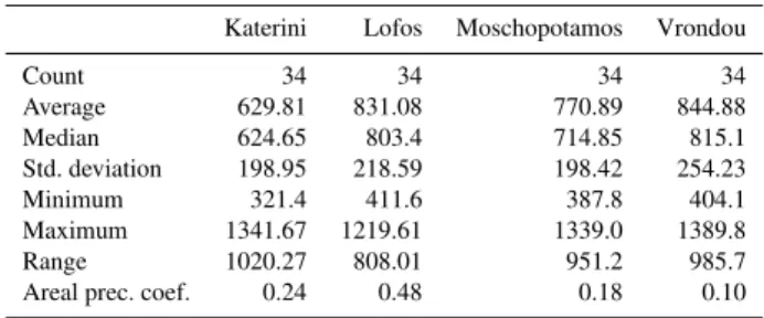
Table 2. Summary statistics of the annual precipitation time series (mm).
Katerini Lofos Moschopotamos Vrondou
Count 34 34 34 34
Average 629.81 831.08 770.89 844.88
Median 624.65 803.4 714.85 815.1
Std. deviation 198.95 218.59 198.42 254.23
Minimum 321.4 411.6 387.8 404.1
Maximum 1341.67 1219.61 1339.0 1389.8
Range 1020.27 808.01 951.2 985.7
Areal prec. coef. 0.24 0.48 0.18 0.10
Pieria and constitutes the greatest receiver of surface water. The primary economic activity in this area is agriculture, re-sulting in high irrigation needs. As drought affects the farm-ers’ choice of irrigation systems (Schuck et al., 2005), an in-vestigation of the regional drought conditions is considered as a prerequisite for adopting more technically efficient irri-gation systems, especially during low precipitation periods. In this study, precipitation measurements from four existing stations have been used: Katerini, Lofos, Moschopotamos and Vrondou. Their coordinates and elevations are presented in Table 1, while their locations are displayed in Fig. 1.
The stations have a common period of monthly data last-ing 34 yr, from 1974 to 2007. Basic summary statistics for the annual time series are presented in Table 2. The areal precipitation is calculated in a GIS environment through a modified Thiessen method where polygons are created ac-cording to both distance and elevation minimization. These polygons provide weight coefficients (Table 2) that show the influence of every individual station on the Aison Basin re-lated to distance and elevation criteria.
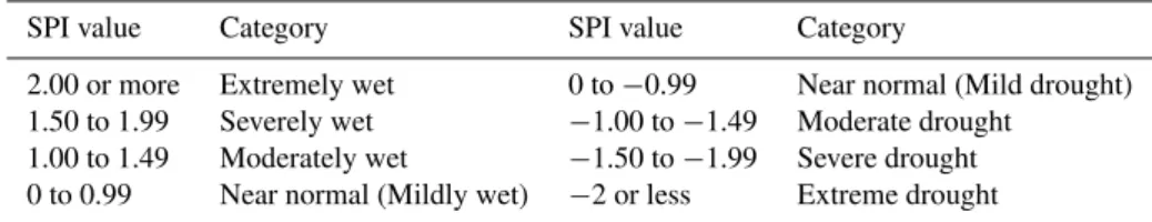
Table 3.Drought classification by SPI value.
SPI value Category SPI value Category
2.00 or more Extremely wet 0 to−0.99 Near normal (Mild drought) 1.50 to 1.99 Severely wet −1.00 to−1.49 Moderate drought
1.00 to 1.49 Moderately wet −1.50 to−1.99 Severe drought 0 to 0.99 Near normal (Mildly wet) −2 or less Extreme drought
3 Methods
The Standardized Precipitation Index (SPI), developed by McKee et al. (1993), quantifies precipitation deficit for mul-tiple timescales. The SPI relies on a long-term precipitation record for a desired region, “ideally a continuous period of at least 30 yr” (McKee et al., 1993). Moreover, a 30-yr pe-riod is practically considered an adequately large data sample for which reliable estimates can be determined (Arguez and Vose, 2011). Monthly precipitation values accumulated for the time scale of interest are fitted to a probability distribu-tion, which is then transformed to the standard normal ran-dom variablezwith mean as zero and variance as one. The zscore is the value of the SPI. Positive SPI values indicate greater than mean precipitation, while negative values indi-cate less than mean precipitation. Because the SPI is stan-dardized, wetter and drier climates can be represented in the same way. Wet periods can also be monitored using SPI.
The classification system shown in Table 3 (McKee et al., 1993) is used to define the strength of the precipitation anomaly. The SPI value of−1 is commonly used as thresh-old for drought event definition (Cancelliere et al., 2005). The duration of the drought event is defined by its beginning and end, while its severity is the accumulated SPI values for the duration of the event and its intensity is measured as the drought severity divided by the drought duration.
Computation of the SPI involves fitting a gamma probabil-ity distribution to a given frequency distribution of precipita-tion totals for a staprecipita-tion. The gamma distribuprecipita-tion is considered to fit well to monthly precipitation time series and was orig-inally used in the development of the SPI method. However, other distributions can also be used if they better fit a partic-ular time series (Guttman, 1999). An extended description of the method used for the SPI computation can be found in Edwards and McKee (1997).
Two-dimensional (2-D) and three-dimensional (3-D) log-linear models have been successfully used to model the ex-pected frequencies of class transitions of SPI values and served as a tool for short-term forecasting of drought. Paulo et al. (2005) used 2-D loglinear models to fit drought class transitions matrices constructed for several sites in south-ern Portugal. Based on SPI values, four drought classes were considered: non drought (SPI≥0), mild drought (−1<SPI<0), moderate drought (−1.5<SPI≤ −1) and severe or extreme drought (SPI≤ −1.5). The computed
odds and respective confidence intervals were used to predict drought class transitions one month ahead, given the drought class of a certain month. The 2-D quasi-association model sufficiently fitted five of the data series used, while the 2-D quasi-symmetry model was selected for two series.
Moreira et al. (2008) extended the work of Paulo et al. (2005) using the same drought classification and 3-D log-linear models to predict drought class transitions one month ahead, given the drought class for the last two months, which also allows for extending the prediction to two months ahead. The quasi-association model adequately fitted their data (14 sites in southern Portugal).
In the present work, a 3-D loglinear models approach was used to investigate drought class transitions in the Aison River Basin, based on the SPI values computed on a 12-month time scale. Since in our study the SPI value of−1 was the threshold for the definition of drought, the four drought classes used were non drought (SPI>−1), moderate drought (−1.5<SPI≤ −1.0), severe drought (−2<SPI≤ −1.5) and extreme drought (SPI≤ −2).
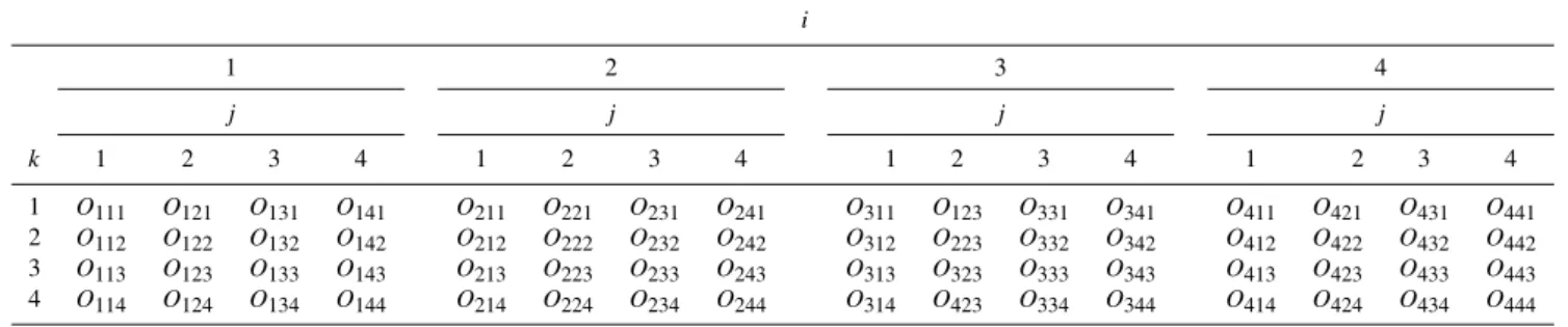
The aim of this analysis is knowing the drought class of two consecutive months to predict the drought class for the following month. For this purpose a 3-dimension contin-gency table is constructed for each station and for the areal time series. A 3-D contingency table has three categories (A,B,C) representing the three consecutive months (t−2, t−1 and t, respectively). Each category has a level (i,j,k forA,B,C,respectively). The level of a category (month) represents its drought class (1=non drought, 2=moderate drought, 3=severe drought and 4=extreme drought). Each cell of the contingency table shows the observed counts of the transitions between the levels of the three categories, as displayed in Table 4. For example, O421 is the number of the occurrences of the three consecutive months with drought classes 4, 2 and 1, respectively.
The construction of the contingency table is based on the assumption that the monthly SPI series are homogeneous and disregards which months the 3-month sequence involves. Loglinear models with Poisson sampling (Agresti, 2002) are used to fit the observed frequencies Oij k and estimate the corresponding expected frequencies Eijk.
Table 4.Three-dimensional contingency table of observed drought class transitionsOij k.
i
1 2 3 4
j j j j
k 1 2 3 4 1 2 3 4 1 2 3 4 1 2 3 4
1 O111 O121 O131 O141 O211 O221 O231 O241 O311 O123 O331 O341 O411 O421 O431 O441 2 O112 O122 O132 O142 O212 O222 O232 O242 O312 O223 O332 O342 O412 O422 O432 O442 3 O113 O123 O133 O143 O213 O223 O233 O243 O313 O323 O333 O343 O413 O423 O433 O443 4 O114 O124 O134 O144 O214 O224 O234 O244 O314 O423 O334 O344 O414 O424 O434 O444
Table 5.Selected loglinear quasi-association submodels for all sites.
Site Selected submodel RD df p-value
Katerini logEij k=λ+λiA+λBj +λCk +βuivj+ηvjwk+δ4I (i=j=k) 35.774 51 0.948
Lofos logEij k=λ+λ
A
i +λBj +λCk+βuivj+αuiwk+ηvjwk+τ uivjwk
+δ4I (i=j=k) 44.262 49 0.665
Moschopotamos logEij k=λ+λAi +λBj+λCk +βuivj+ηvjwk+τ uivjwk+δ2I (i=k) 31.204 50 0.983
Vrondou logEij k=λ+λ A
i +λBj +λCk+βuivj+αuiwk+ηvjwk+τ uivjwk +δ1I (i=j )+δ3I (j=k)
38.994 49 0.846
Aison basin logEij k=λ+λ A
i +λBj +λCk+βuivj+αuiwk+ηvjwk+τ uivjwk +δ4I (i=j=k)
42.231 49 0.742
al. (2006, 2008). The general form of this model is given by the following equation:
logEij k=λ+λAi +λBj +λCk +βuivj+αuiwk
+ηvjwk+τ uivjwk+ +δ1iI (i=j )+δ2iI (i=k)
+δ3jI (j=k)+δ4iI (i=j=k)
(1)
whereEij kis the expected frequency;A,BandCare the cat-egories corresponding to three consecutive monthst−2,t−1 andt,i,j andkǫ{1,2,3,4} :1→non drought, 2→ moder-ate drought, 3→severe drought, 4→extreme drought.λis the constant term of the model;λAi ,λBj,λCk represent thei-th, j-th,k-th levels for categoriesA,B,C, respectively; ui,vj, wkare thei-th,j-th,k-th level scores of categoriesA,B,C, respectively, usually taken asui=i,vj=j,wk=k,β,α,η, τ are linear association parameters;δ1i ,δ2i ,δ4i are param-eters associated to the i-th diagonal element of categoryA; δ3j is a parameter associated with thej-th diagonal element of categoryB, andI is an indicator function defined as: I (condition)=
1 if condition is true
0 if condition is false (2)
This model comprises two components: (a) the linear-by-linear association model consisting of the first eight terms and (b) the rest four terms describing the effect of the di-agonal elements of the 3-D contingency table. These four terms reflect the persistency of drought in the same class for
consecutive months. The persistency of each drought class is associated with a different parameter value. For example having the first two months in drought class 1 (i=j=1) is associated with the parameterδ11, while having the first two months in drought class 2 (i=j=2) is associated with the parameterδ12. As a result, a maximum of 16 parameters are needed to account for drought class persistency.
Since the homogenous form of the second component of the model is more suitable for ordered variables (Lawal, 2003), which is our case, the following simplified form of the equation of the model (Eq. 1) is proposed:
logEij k=λ+λAi +λBj+λCk +βuivj+αuiwk
+ηvjwk+τ uivjwk+ +δ1I (i=j )+δ2I (i=k)
+δ3I (j=k)+δ4I (i=j=k)
(3)
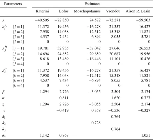
Table 6.Estimated parameter values.
Parameters Estimates
Katerini Lofos Moschopotamos Vrondou Aison R. Basin
λ −40.505 −72.850 74.572 −72.271 −59.503
λAi [i=1] 11.372 19.456 −16.278 21.357 16.427
[i=2] 7.958 14.038 −12.512 15.318 11.821
[i=3] 4.537 7.434 −6.894 8.055 5.781
[i=4] 0 0 0 0 0
λBj [j=1] 19.781 32.935 −37.042 27.646 26.553
[j=2] 14.694 24.852 −29.659 20.687 19.956
[j=3] 8.618 13.489 −16.446 11.101 10.426
[j=4] 0 0 0 0 0
λCk [k=1] 11.372 19.456 −16.278 21.357 16.427
[k=2] 7.958 14.038 −12.512 15.318 11.821
[k=3] 4.537 7.434 −6.894 8.055 5.781
[k=4] 0 0 0 0 0
β 1.294 2.726 −3.055 2.504 2.174
α 0.811 1.620 0.727
η 1.294 2.726 −3.055 2.504 2.174
τ −0.419 0.358 −0.536 −0.327
δ1 0.764
δ2 0.728
δ3 0.764
δ4 1.142 0.868 1.051
By default, due to the definition of the SPI and the relevant classification system, moderate, severe and extreme droughts (classes 2, 3, 4) comprise a relatively small portion of the SPI time series (McKee et al., 1993). Although they exhibit a similar trend for persistency with class 1, as it was observed in our data series, the numbers of the relevant observed fre-quencies are small. Hence, homogenizing drought class per-sistency and reducing the number of estimated parameters resulted in models that fitted the data better than model (1) in all our cases. Thus, in this work, a quasi-association model with homogenous diagonal effect was considered more ap-propriate to describe the observed drought class transitions.
The goodness of fit of a loglinear model is tested by a chi-square test performed on the value of the residual deviance (RD) of the model:
RD=2X i
X
j X
k
Oij klog O
ij k
Eij k
(4) The residual deviance has an approximate chi-square distri-bution with degrees of freedom equal to the number of the cells of the contingency table minus the number of linearly independent estimated model parameters. If the p-value of a model exceeds a chosen level of significanceα(in our case α=0.05), then the null hypothesis that the model fits well to the data is not rejected.
Model (3) fitted adequately all data series studied in the present work. For each station, an alternative submodel was selected, including only the most significant parame-ters through the backward elimination method. The selected submodels and the respective residual deviance, degrees of freedom (df) and p-value of the submodel are presented in Table 5. The parameters of the selected submodels were esti-mated by the maximum likelihood method. Their values are presented in Table 6. The software used for model fitting was SPSS 17.
The analysis and forecast of the drought class transition probabilities are based on the odds of the estimated expected frequencies. Odds are ratios of expected frequencies, as de-fined by the following equation:
kl|ij= Eij k Eij l
,k6=l (5)
Odds represent how more probable an event is to occur instead of another. Equation (5) means that, given that a site was in drought classiat montht−2 and in classj at month t−1, it iskl|ij times more probable that at montht, it will be in classkthan in classl.
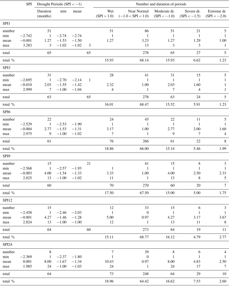
Table 7.Areal precipitation – drought analysis results for all time scales.
SPI Drought Periods (SPI<−1) Number and duration of periods
Duration min mean Wet Near Normal Moderate dr. Severe dr. Extreme dr. (months) (SPI>1.0) (−1.0<SPI<1.0) (SPI<−1.0) (SPI<−1.5) (SPI<−2.0)
SPI1
number 51 51 86 51 21 5
min −2.742 1 −2.74 −2.74 1 1 1 1 1
mean −0.001 1.27 −1.53 −1.50 1.27 3.23 1.27 1.29 1.00
max 3.283 3 −1.02 −1.02 3 13 3 3 1
total 65 65 278 65 27 5
total % 15.93 68.14 15.93 6.62 1.23
SPI3
number 31 28 41 31 15 5
min −2.695 1 −2.70 −2.14 1 1 1 1 1
mean −0.010 2.03 −1.55 −1.42 2.32 1.00 2.03 1.60 1
max 2.999 7 −1.00 −1.04 4 1 7 4 1
total 63 65 278 63 24 5
total % 16.01 68.47 15.52 5.91 1.23
SPI6
number 22 24 45 22 11 5
min −2.529 1 −2.53 −1.90 1 1 1 1 1
mean −0.004 2.77 −1.53 −1.31 3.17 1.00 2.77 2.00 1.60
max 2.975 9 −1.00 −1.02 7 1 9 7 4
total 61 76 266 61 22 8
total % 18.86 66.00 15.14 5.46 1.99
SPI9
number 15 21 41 15 8 3
min −2.568 1 −2.57 −1.93 1 1 1 1 1
mean −0.003 4.00 −1.54 −1.33 3.33 1.00 4.00 2.50 2.33
max 2.825 13 −1.00 −1.02 11 1 13 8 5
total 60 70 270 60 20 7
total % 17.50 67.50 15.00 5.00 1.75
SPI12
number 15 12 33 15 6 3
min −2.458 1 −2.46 −2.03 1 0 1 1 1
mean −0.001 4.27 −1.46 −1.28 5.00 0.97 4.27 3.17 3.67
max 2.824 13 −1.00 −1.00 12 1 13 11 8
total 64 60 273 64 19 11
total % 15.11 68.77 16.12 4.79 2.77
SPI24
number 8 7 39 8 6 4
min −2.369 1 −2.37 −1.80 1 0 1 1 1
mean 0.001 8.00 −1.67 −1.34 10.43 0.97 8.00 4.83 2.50
max 1.985 24 −1.00 −1.03 24 1 24 17 7
total 64 73 248 64 29 10
Table 8.Maximum values of drought characteristics for all stations and time scales.
max severity max intensity max duration
value month value period value period
SPI1
Katerini −2.41 Aug 1992 −2.11 Oct 1989 3 Nov 2006–Jan 2007
Lofos −2.30 May 2002 −2.17 May 2006 4 Jun 2000–Sep 2000
Moschopotamos −2.51 Sep 2001 −2.51 Sep 2001 3 Feb 1989–Apr 1989
Vrondou −2.61 Apr 1986 −2.61 Apr 1986 3 Jun 2000–Aug 2000
Aison Basin −2.74 Sep 2001 −2.74 Sep 2001 3 Jun 2000–Aug 2000
SPI3
Katerini −2.45 Jan 2007 −2.01 May 2000–Aug 2000 8 Oct 1989–May 1990
Lofos −2.93 Sep 2000 −2.87 Aug 2000–Sep 2000 7 Oct 1989–Apr 1990
Moschopotamos −3.05 Apr 1989 −2.54 Mar 1989–May 1989 6 Jan 1977–Jun 1977
Vrondou −2.51 Jan 2007 −1.85 Jun 1988–Sep 1988 8 Oct 1989–May 1990
Aison Basin −2.70 Jan 2007 −2.14 Jun 2005 7 Oct 1989–Apr 1990
SPI6
Katerini −2.78 Aug 2000 −2.13 Jun 2000–Sep 2000 9 Nov 1989–Jul 1990
Lofos −2.60 Jan 1990 −1.88 Nov 1989–Jul 1990 9 Nov 1989–Jul 1990
Moschopotamos −2.30 Oct 1984 −1.60 Feb 1977–Aug 1977 8 Dec 1989–Jul 1990
Vrondou −2.40 Sep 1988 −1.82 Nov 1989–Jul 1990 9 Nov 1989–Jul 1990
Aison Basin −2.53 Mar 1990 −1.90 Nov 1989–Jul 1990 9 Nov 1989–Jul 1990
SPI9
Katerini −2.73 Aug 1977 −1.88 Oct 1989–Sep 1990 12 Oct 1989–Sep 1990
Lofos −2.51 Apr 1990 −1.92 Aug 2000–Sep 2000 13 Sep 1989–Sep 1990
Moschopotamos −2.10 Jun 1990 −1.81 Apr 1977–Dec 1977 13 Sep 1989–Sep 1990
Vrondou −2.48 Apr 1990 −1.70 Aug 1989–Sep 1990 14 Aug 1989–Sep 1990
Aison Basin −2.57 Apr 1990 −1.93 Aug 2000–Sep 2000 13 Sep 1989–Sep 1990
SPI12
Katerini −2.47 Jul 1990 −2.07 Dec 1989–Nov 1990 12 Dec 1989–Nov 1990
Lofos −2.44 Mar 1990 −1.96 Nov 1989–Nov 1990 13 Nov 1989–Nov 1990
Moschopotamos −2.61 Nov 1977 −1.78 Nov 1989–Oct 1990 12 Nov 1989–Oct 1990
Vrondou −2.37 Mar 1990 −1.81 Oct 1989–Dec 1990 15 Oct 1989–Dec 1990
Aison Basin −2.46 Mar 1990 −2.03 Nov 1989–Nov 1990 13 Nov 1989–Nov 1990
SPI24
Katerini −2.47 Apr 1990 −1.58 Apr 1989–Dec 1991 33 Apr 1989–Dec 1991
Lofos −2.50 Nov 2001 −1.67 Sep 1989–Mar 1991 19 Sep 1989–Mar 1991
Moschopotamos −2.18 Aug 1978 −1.67 Jan 1998–Oct 1998 24 Mar 1989–Feb 1991
Vrondou −2.52 Apr 1990 −1.71 Oct 1988–Oct 1991 37 Oct 1988–Oct 1991
Aison Basin −2.37 Apr 1990 −1.80 Apr 1989–Mar 1991 24 Apr 1989–Mar 1991
Poisson sampling an estimator of the standard error is p
Var(logkl|ij). For the general form of the model applied in this work (Eq. 3):
logkl|ij=logEij k−logEij l=
=λCk −λCl +αui(wk−wl)+ηvj(wk−wl)
+τ uivj(wk−wl)
+δ2I (i=k)−δ2I (i=l)+δ3I (j=k)−δ3I (j=l)
+δ4I (i=j=k)−δ4I (i=j=l)
(6)
Equation (6) was used for the calculation of the variance of the logarithm of odds, since all the terms in the right hand side of this equation are known and the variances and covari-ances of the estimated parameters were computed as part of the model fitting process.
The upper and lower bounds of the log-odds asymptotic confidence interval with probability 1-a can be estimated as: logkl|ij±z1−α/2
q
Var(logkl|ij) (7)
wherez1−α/2is the 1-α/2 quantile of a standard normal vari-able.
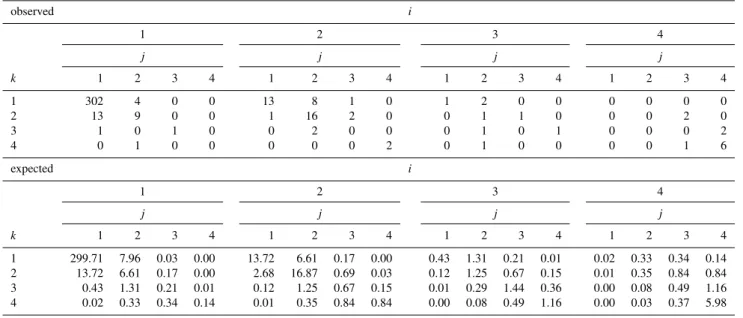
Table 9.Observed and expected drought class transitions for the Aison River Basin.
observed i
1 2 3 4
j j j j
k 1 2 3 4 1 2 3 4 1 2 3 4 1 2 3 4
1 302 4 0 0 13 8 1 0 1 2 0 0 0 0 0 0
2 13 9 0 0 1 16 2 0 0 1 1 0 0 0 2 0
3 1 0 1 0 0 2 0 0 0 1 0 1 0 0 0 2
4 0 1 0 0 0 0 0 2 0 1 0 0 0 0 1 6
expected i
1 2 3 4
j j j j
k 1 2 3 4 1 2 3 4 1 2 3 4 1 2 3 4
1 299.71 7.96 0.03 0.00 13.72 6.61 0.17 0.00 0.43 1.31 0.21 0.01 0.02 0.33 0.34 0.14 2 13.72 6.61 0.17 0.00 2.68 16.87 0.69 0.03 0.12 1.25 0.67 0.15 0.01 0.35 0.84 0.84 3 0.43 1.31 0.21 0.01 0.12 1.25 0.67 0.15 0.01 0.29 1.44 0.36 0.00 0.08 0.49 1.16 4 0.02 0.33 0.34 0.14 0.01 0.35 0.84 0.84 0.00 0.08 0.49 1.16 0.00 0.03 0.37 5.98
4 Results and discussion
SPI values, based on the monthly precipitation time series, for 1-, 3-, 6-, 9-, 12- and 24-month aggregation time scales were used for drought analysis in the study area of Pieria. The SPI value of−1 was selected as the critical value for the definition of drought events. For the computation of the SPI values, all precipitation time series were assumed to be gamma distributed. The results of the drought analysis for the Aison River Basin (areal precipitation) are presented in Table 7.
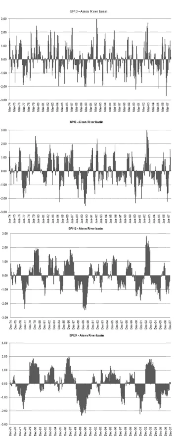
Different aggregation time scales were used, as they re-flect drought impacts on different types of water resources. For all time scales, it can be seen in Table 7 that 30–45 % of the total number of months with SPI<−1 belong to se-vere or extreme drought classes. In most of the cases and especially for small time scales, SPI values remained nega-tive after the termination of a drought event, sometimes for the whole period until the initiation of the next drought event. Usually, on larger time scales the two events and the period in between were considered as a continuous drought episode. Consequently, longer aggregation time scales led to less but more persisting drought events, as it is evident in the follow-ing graphs of SPI3, SPI6, SPI12 and SPI24 for the Aison River Basin in Fig. 2 (SPI9 graph is omitted due to space limitations). This should be taken into account when SPI is used as a drought indicator in the context of a drought mon-itoring and early warning system, where certain SPI values are selected as triggers for drought management. Although the value of−1 is frequently used as the threshold defining the initiation and termination of a drought event, it should not be considered as the trigger for ending an issued warning or a drought management action.
According to the applied drought event definition, the SPI value can become negative without a drought necessarily oc-curring. In Fig. 2, it can be noted that as the time scale increases, the percent of the times that a negative SPI re-sults in drought (SPI<−1) decreases. For example, 53 % of the times the SPI3 goes below zero result in drought. This percentage is 44 %, 41 % and 34 % for the SPI6, SPI12 and SPI24, respectively.
Table 8 summarises for each drought characteristic its maximum value and the period this value was recorded, for all stations and aggregation time scales.
Among the identified drought periods at the local and re-gional level, the period from October 1988 to July 1991 is pointed out as it includes almost all the drought events with maximum duration (for all stations and all aggregation time scales), and also most of the drought events with maxi-mum intensity, especially in aggregation time scales equal or greater than six months. During this period, almost the whole Greek territory suffered from severe or extreme droughts (Li-vada and Assimakopoulos, 2007). Similar drought condi-tions were also observed in Italy (Rossi and Somma, 1995). Other significant drought periods that were also identified have an impact degree depending on the time scale and site location. The drought period around the middle of the 1970s was also reported by Loukas and Vasiliades (2004) in their work concerning the region of Thessaly in Greece, which is located southwest of the present study area.
Fig. 2.SPI values of variable time scales for the Aison River Basin.
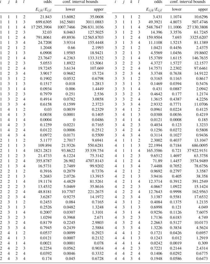
The odds of the expected frequencies and the respective confidence intervals of these odds, which serve as a tool for short-term drought forecasting, were computed for all sites. In Table 10 odds and confidence intervals for the Aison River basin data set are presented.
From a total of 96 odds for each site (all possible combina-tions), the number of confidence intervals, not including the unit, was 71 for Katerini, 70 for Lofos, 78 for Moschopota-mos, 60 for Vrondou and 59 for the areal precipitation data series. The results were quite satisfying, considering the fact that due to the small number of the defined drought events, many of the three month drought class combinations had an observed frequency equal to zero. For the Aison River Basin data set, for instance, zero observed frequencies were 38 out of 64 (see Table 9).
Based on the computed odds and respective confidence in-tervals, all possible combinations of drought classes for two consecutive months (t−1,t) and the most probable drought class for the following month (t+1), for each data series, are presented in Table 11.
According to Table 11, smooth drought class transitions appear to be more probable than transitions to classes two or three levels more (or less) severe. Also, in most of the cases the second month’s drought class is preserved in the third month. These conclusions are in accordance with the results of former studies (Paulo et al., 2005; Mishra et al., 2007; Moreira et al., 2008) and with the fact that droughts usually do not initiate or come to an end suddenly.
5 Concluding remarks
In the present work, the frequency, duration and severity of meteorological drought in the Aison River Basin were analysed using the SPI computed on variable time scales. Monthly precipitation time series from four meteorological stations operating in the study area and the areal precipitation resulting from them composed the data sets for this analysis. A number of drought events of different classes were de-fined for all the time scales at the local (sites) and basin scale. Most of them belonged to the moderate drought class, but “extreme drought” events were also identified. Especially, during the period from October 1988 to July 1991, the study area suffered the longest-lasting and most severe drought. Also, most of the months with maximum drought intensity were observed in this time period.
Table 10.Odds and respective confidence intervals for the Aison River Basin.
i j k l odds conf. interval bounds i j k l odds conf. interval bounds
Eij k/Eij l lower upper Eij k/Eij l lower upper
1 1 1 2 21.843 13.6082 35.0608 3 1 1 2 3.431 1.1074 10.6296
1 1 1 3 699.6305 162.5601 3011.0883 3 1 1 3 49.3921 4.8073 507.4746
1 1 1 4 17 295.3904 1007.7466 296 831.1036 3 1 1 4 548.7847 11.1006 27 130.3808
1 1 2 3 32.03 8.0463 127.5025 3 1 2 3 14.396 3.3576 61.7245
1 1 2 4 791.8061 49.8936 12 565.8703 3 1 2 4 159.9504 7.693 3325.6207
1 1 3 4 24.7208 3.9314 155.4448 3 1 3 4 11.1108 1.5215 81.1389
1 2 1 2 1.2048 0.66 2.1993 3 2 1 2 1.0421 0.4456 2.4375
1 2 1 3 6.0908 1.9585 18.9421 3 2 1 3 4.5569 1.0456 19.8602
1 2 1 4 23.7647 4.2363 133.3152 3 2 1 4 15.3789 1.6115 146.7635
1 2 2 3 5.0553 1.8922 13.5061 3 2 2 3 4.3727 1.5727 12.1577
1 2 2 4 19.7245 3.6134 107.669 3 2 2 4 14.7571 2.2302 97.6461
1 2 3 4 3.9017 0.9682 15.724 3 2 3 4 3.3748 0.7638 14.9122
1 3 1 2 0.1902 0.0532 0.6798 3 3 1 2 0.3165 0.1163 0.8617
1 3 1 3 0.1517 0.018 1.2813 3 3 1 3 0.1469 0.0394 0.5476
1 3 1 4 0.0934 0.006 1.4449 3 3 1 4 0.431 0.0887 2.0942
1 3 2 3 0.7979 0.251 2.536 3 3 2 3 0.4642 0.177 1.2174
1 3 2 4 0.4914 0.0782 3.0858 3 3 2 4 1.3615 0.4387 4.2256
1 3 3 4 0.6158 0.1599 2.3723 3 3 3 4 2.9332 0.7771 11.0706
1 4 1 2 0.03 0.0039 0.2329 3 4 1 2 0.0961 0.0224 0.4125
1 4 1 3 0.0038 0.0001 0.1405 3 4 1 3 0.0388 0.0036 0.4219
1 4 1 4 0.0004 0 0.0486 3 4 1 4 0.0121 0.0008 0.185
1 4 2 3 0.1259 0.0221 0.7165 3 4 2 3 0.4034 0.123 1.3233
1 4 2 4 0.0122 0.0006 0.2512 3 4 2 4 0.1256 0.0272 0.5808
1 4 3 4 0.0972 0.0171 0.5509 3 4 3 4 0.3114 0.1027 0.9436
2 1 1 2 5.1177 2.7017 9.6941 4 1 1 2 2.3002 0.4037 13.1047
2 1 1 3 109.894 21.9326 550.6281 4 1 1 3 22.1994 0.7184 686.0095
2 1 1 4 1821.2821 93.8622 35 339.754 4 1 1 4 165.3586 0.721 37 922.9151
2 1 2 3 21.4733 6.1224 75.3142 4 1 2 3 9.6512 1.4697 63.3758
2 1 2 4 355.8787 26.902 4707.8143 4 1 2 4 71.89 1.4457 3574.9489
2 1 3 4 16.5731 2.7489 99.9202 4 1 3 4 7.4488 0.7052 78.6756
2 2 1 2 0.3916 0.2079 0.7376 4 2 1 2 0.9692 0.2797 3.3587
2 2 1 3 5.2683 2.0726 13.3915 4 2 1 3 3.9416 0.405 38.358
2 2 1 4 19.1174 4.4829 81.5261 4 2 1 4 12.3714 0.3912 391.2549
2 2 2 3 13.4532 5.0469 35.8616 4 2 2 3 4.0667 1.0922 15.1424
2 2 2 4 48.8181 10.7707 221.2675 4 2 2 4 12.7643 0.9998 162.9563
2 2 3 4 3.6287 0.9275 14.1972 4 2 3 4 3.1387 0.5581 17.6532
2 3 1 2 0.2453 0.084 0.7165 4 3 1 2 0.4084 0.1375 1.2135
2 3 1 3 0.2526 0.0482 1.3248 4 3 1 3 0.6998 0.121 4.049
2 3 1 4 0.2007 0.0307 1.3101 4 3 1 4 0.9256 0.1126 7.6075
2 3 2 3 1.0294 0.3968 2.671 4 3 2 3 1.7136 0.6183 4.749
2 3 2 4 0.8179 0.2245 2.9803 4 3 2 4 2.2663 0.5127 10.0173
2 3 3 4 0.7945 0.2439 2.5884 4 3 3 4 1.3226 0.3834 4.5624
2 4 1 2 0.0537 0.0099 0.2923 4 4 1 2 0.1721 0.0426 0.6957
2 4 1 3 0.0121 0.0007 0.2132 4 4 1 3 0.1243 0.012 1.2919
2 4 1 4 0.0021 0.0001 0.078 4 4 1 4 0.0242 0.0019 0.309
2 4 2 3 0.2254 0.0562 0.9034 4 4 2 3 0.7221 0.2144 2.4314
2 4 2 4 0.0392 0.0046 0.3332 4 4 2 4 0.1406 0.0292 0.6775
Table 11.Most probable drought class for montht+1, given the drought classes of the two previous months (t−1,t).
Katerini Lofos Moschopotamos Vrondou Aison R. Basin
t-1 t t+1 t+1 t+1 t+1 t+1
1 1 1 1 1 1 1
1 2 1 2, 1 2, 1 2, 1 2, 1
1 3 1, 2, 3, 4 2, 3, 4 3, 4 2, 3, 4 2, 3, 4
1 4 4, 3 4 4 4 4
2 1 1 1 1 1 1
2 2 2, 1 2 2, 1 2 2
2 3 1, 2, 3, 4 2, 3, 4 2, 3, 4 3 2, 3, 4
2 4 4, 3 4 4 4 4
3 1 1 1 1 1, 2 1
3 2 1 1, 2 1 2 1, 2
3 3 3 3 3 3 2, 3, 4
3 4 4, 3 4, 3 4, 3 4 4
4 1 1 1, 2 1 1, 2, 3, 4 1, 2
4 2 1 2, 3, 1 1 2, 3, 4 1, 2, 3, 4
4 3 1, 2, 3, 4 1, 2, 3, 4 1, 2, 3, 4 3, 2 1, 2, 3, 4
4 4 4 4, 3 4, 3 1, 2, 3, 4 4
Short-term forecasting of droughts was based on the odds of the expected frequencies of drought class transitions and the respective confidence intervals. The 3-D loglinear quasi-association model with homogenous diagonal effect pro-posed in this study fitted adequately to the observed data sets. The expected class transition frequencies for each data set were successfully estimated by an adapted submodel selected through the backward elimination model. The odds of the ex-pected frequencies and their confidence intervals could reli-ably predict the drought class transitions one or two months ahead, given the drought classes of the last two months, in most of the cases. The results of short-term forecasting ap-proach showed that smooth drought severity class transitions appear to be more probable than abrupt ones.
Based on the quality of the results, the proposed approach, with a continuous update of precipitation records, could be regarded as a useful tool for regional water resources man-agers and irrigators for drought analysis and short-term warn-ing at the farm and basin scale. Towards this direction, an up-graded network of on-line meteorological stations has been recently established in the Aison River Basin, supporting the viability and any future extension of the proposed models as well, as the reliability of results.
Acknowledgements. This research was supported by the Program Interreg III B- MEDOCC through the project MEDDMAN – “Integrated water resources management, development and confrontation of common and transnational methodologies for combating drought within the MEDOCC region”.
Edited by: N. R. Dalezios
Reviewed by: G. Karantounias and G. Rossi
References
Agresti, A.: Categorical Data Analysis, Second Edition, Wiley Se-ries in Probability and Statistics, John Wiley & Sons Inc., Hobo-ken, New Jersey, 710 pp., 2002.
Arguez, A. and Vose, R. S: The Definition of the Standard WMO Climate Normal: The Key to Deriving Alternative Climate Nor-mals, B. Amer. Meteorol. Soc., 92, 699–704, 2011.
Cancelliere, A., Bonaccorso, B., Cavallaro, L., and Rossi G.: Re-gional Drought Identification Module REDIM, Department of Civil and Environmental Engineering, University of Catania, Catania, Italy, 43 pp., 2005.
Cancelliere, A., Di Mauro, G., Bonaccorso, B., and Rossi, G.: Drought forecasting using the Standardized Precipitation Index, Water Resour. Manage., 21, 801–819, 2007.
Dai, A.: Drought under global warming: a review, WIREs, Climate Change, 2, 45–65, 2011.
Dracup, J. A., Lee, K. S., and Paulson Jr., E. G.: On the Definition of Droughts, Water Resour. Res., 16, 297–302, 1980.
Edossa, D. C., Babel, M. S., and Gupta, A. D.: Drought in the Awash River Basin, Ethiopia, Water Resour. Manag., 24, 1441– 1460, 2010.
Edwards, D. C. and McKee, T. B.: Characteristics of 20th Cen-tury Drought in the United States at Multiple Time Scales, At-mospheric Science Paper No. 634, Climatology Report No. 97-2, Colorado State University, Fort Collins, Colorado, 155 pp., 1997. Guttman, N. B.: Comparing the Palmer Drought Severity Index and the Standardized Precipitation Index, J. Am. Water Resour. As-soc., 34, 113–121, 1998.
Guttman, N. B.: Accepting the Standardized Precipitation Index, A calculation algorithm, J. Am. Water Resour. Assoc., 35, 311– 322, 1999.
Hisdal, H. and Tallaksen, L. M.: Drought Event Definition, ARIDE Technical Report No. 6, Department of Geophysics, University of Oslo, Oslo, 41 pp., 2000.
Hwang, Y. and Carbone, G.: Ensemble Forecasts of Drought In-dices Using a Conditional Residual Resampling Technique, J. Appl. Meteorol., 48, 1289–1301, 2009.
Lawal, H. B.: Categorical data analysis with SAS and SPSS ap-plications, Lawrence Erlbaum Associates, New Jersey, 561 pp., 2003.
Livada, I. and Assimakopoulos, V. D.: Spatial and temporal analysis of drought in Greece using the Standardized Precipitation Index (SPI), Theor. Appl. Climatol., 89, 143–153, 2007.
Loukas, A. and Vasiliades, L.: Probabilistic analysis of drought spatiotemporal characteristics in Thessaly region, Greece, Nat. Hazards Earth Syst. Sci., 4, 719–731, doi:10.5194/nhess-4-719-2004, 2004.
McKee, T. B., Doesken, N. J., and Kleist, J.: The relationship of drought frequency and duration to time scale, Eighth Conference on Applied Climatology, Anaheim, CA, 179–186, 1993. Mishra, A. K. and Singh, V. P.: A review of drought concepts, J.
Hydrol., 391, 202–216, 2010.
Mishra, A. K., Desai, V. R., and Singh, V. P.: Drought Forecasting Using a Hybrid Stochastic and Neural Network Model, J. Hydrol. Eng., 12, 626–638, 2007.
Mishra, A. K., Singh, V. P., and Desai, V. R.: Drought characteriza-tion: a probabilistic approach, Stoch. Environ. Res. Risk Assess., 23, 41–55, 2008.
Moreira, E. E., Paulo, A. A., Pereira, L. S., and Mexia, J. T.: Anal-ysis of SPI drought class transitions using loglinear models, J. Hydrol., 331, 349–359, 2006.
Moreira, E. E., Coelho, C. A., Paulo, A. A., Pereira, L. S., and Mexia, J. T.: SPI-based drought category prediction using log-linear models, J. Hydrol., 354, 116–130, 2008.
Paulo, A. A. and Pereira, L. S.: Drought concepts and Characteri-zation, Water Int., 31, 37–49, 2006.
Paulo, A. A., Ferreira, E., Coelho, C. A., and Pereira, L. S.: Drought class transition analysis through Markov and Loglinear models, an approach to early warning, Agr. Water Manage., 77, 59–81, 2005.
Rossi, G.: European Union policy for improving drought prepared-ness and mitigation, Water Int., 34, 441–450, 2009.
Rossi, G. and Somma, F.: Severe drought in Italy: charac-teristics, impact and mitigation strategies. Drought Network News: October 1995, available at: http://drought.unl.edu/ archive/dnn-archive/arch6.pdf, last access: January 2012. Sene, K.: Hydrometeorology, Forecasting and Applications,
Springer, Dordrecht Heidelberg London New York, 355 pp., 2010.
Schuck, E. C., Frasier, W. M., Webb, R. S, Ellingson, L. J., and Umberger, W. J.: Adoption of more technically efficient irriga-tion systems as a drought response, Int. J. Water Resour. Dev., 21, 651–662, 2005.
Wilhite, D. A. and Buchanan-Smith, M.: Drought as Hazard: Un-derstanding the Natural and Social Context, in: Drought and Wa-ter Crises, edited by: Wilhite, D. A., Taylor and Francis Group, New York, 3–32, 2005.