A hybrid approach based on EP and PSO for proficient solving of Unit Commitment Problem

A HYBRID APPROACH BASED ON EP AND PSO FOR PROFICIENT

SOLVING OF UNIT COMMITMENT PROBLEM

R LAL RAJA SINGH*

Research Scholar, Sathyabama University, Chennai

Assistant Professor, Marthandam College of Engineering and Technology, Kuttakuzhi, India. lalrajasinghphd@gmail.com

Dr. C.CHRISTOBER ASIR RAJAN

Associate Professor, Department of Electrical Engineering Pondicherry Engineering College, Pondicherry, India.

Abstract

Unit Commitment Problem (UCP) is a nonlinear mixed integer optimization problem used in the scheduling operation of power system generating units subjected to demand and reserve requirement constraints for achieving minimum operating cost. The task of the UC problem is to determine the on/off state of the generating units at every hour interval of the planning period for optimally transmitting the load and reserve among the committed units. The importance for the necessity of a more effective optimal solution to the UCP problem is increasing with the regularly varying demand. Hereby, we propose a hybrid approach which solves the unit commitment problem subjected to necessary constraints and gives the optimal commitment of the units. The possible combination of demand and their corresponding optimal generation schedule can be determined by the PSO algorithm. Being a global optimization technique, Evolutionary Programming (EP) for solving Unit Commitment Problem, operates on a method, which encodes each unit’s operating schedule with respect to up/down time. When the demand over a time horizon is given as input to the network it successfully gives the schedule of each unit’s commitment that satisfies the demands of all the periods and results in minimum total cost. Because hybridization is dominating, this approach for solving the unit commitment problem is more effective.

Keywords: Generation schedule, Unit commitment problem (UCP), Evolutionary Programming (EP), Particle Swarm Optimization (PSO), Power Flow Constraints (PFC).

1. Introduction

In any power station, investment cost is quite high and the resources required for operating them are quickly becoming inadequate [1]. The cyclic fluctuations in the demand for electricity on a daily and weekly basis has made determination of the best way of meeting these fluctuating demands a problem for the power system [2]. Knowledge of the future demand is a major issue in planning. Accurate forecasting is necessary for the efficient functioning of basic operating functions like thermal and hydrothermal UC, economic dispatch, fuel scheduling and unit maintenance [3]. The production cost for energy varies significantly between different energy sources present in a power system. Moreover a tool is necessary for balancing demand and generation and also for dispatching the generation in an optimal and most economical manner [4].

Power system operators encounter a wide-range of decision-making problems on account of these difficulties. One of the decision making problems is related to the scheduling of the generators at any particular time in a power system. It is not economical to operate all the units necessary to satisfy the peak load during low load periods [5]. The principal aim of a power system is to minimize the power generation expenses while satisfying the hourly forecasted power demand. The UCP method obtains an optimal turn on and turn off schedule for a group of power generation units for each time slot over a given time range [10].

The UCP is an essential area of research which draws more attention from the scientific society due to the fact that even small savings in the operation costs every hour can result in considerable overall economic savings [6]. Unit Commitment (UC) is the best option for determining which of the available power plants should be incorporated for supplying the electricity [7]. UCP is a part of production scheduling which is concerned with the determination of the ON/OFF status of the generating units during each interval of the scheduling period. This is necessary to minimize the cost while meeting the system load and reserve requirements which are open to many types of equipment, system and environmental constraints [8]. The UC should minimize the production cost of the system while satisfying the load demand, spinning reserve, ramp constraints and the operational constraints of the individual units [9].

based on EP-PSO which solves the UCP is detailed in Section 6 with illustrations and mathematical formulations. Section 7 discusses the implementation results and Section 8 concludes the paper.

2. Related works

U.BasaranFilik and M.Kurban [3] have utilized a Fuzzy Logic (FL) method in solving the UC problem of the four-unit Tuncbilek thermal plant of Turkey for an optimum schedule of the generating units subjected to load data constraints forecasted using conventional ANN (ANN) and an improved method which is a combination of ANN and Weighted Frequency Bin Blocks (WFBB). Kaveh Abookazemi et al [8] have presented and identified the alternative strategies with the advantages of Genetic Algorithm for solving the Thermal Unit Commitment (UC) problem. A Parallel Structure has been developed to handle the infeasibility problem in a structured and improved Genetic Algorithm (GA) which provides an effective search and therefore greater economy. Their proposed method leads us to obtain better performance by using both computational methods and classification of unit characteristics. Typical constraints such as system power balance, minimum up and down times, start up and shut-down ramps have been considered. A number of effective parameters related to UC problem have been identified.

S. Prabhakar Karthikeyan et al [9] have proposed an algorithm which solves a security constrained UC problem subjected to both operational and power flow constraints (PFC) and obtains a secure and economical hourly generation schedule. They have adopted an efficient unit commitment (UC) approach with PFC for achieving minimum system operating cost and at the same time satisfying both unit and network constraints with regards to uncertainties. S.Chitra Selvi et al. [13] have presented an innovative approach that utilizes particle swarm optimization technique in solving the Multi- Area Unit Commitment and obtains the optimal or near optimal commitment strategy for the generating units. Their technique has improved efficiency with respect to cost and computation time compared to traditional Dynamic Programming and Evolutionary Programming Methods.Nidul Sinha et al [32] have described the hybridization between PSO and self-adaptive evolutionary programming techniques for solving economic dispatch (ED) problem with non-smooth cost curves where conventional gradient based methods were in-applicable. The convergence capability of evolutionary programming technique was enhanced with hybridization of self-adaptive evolutionary programming technique with PSO intelligence.

D.P. Kothari et al [33] have proposed a hybrid approach consisting of Lagrange Relaxation (LR) and Evolutionary Programming (EP) that maximizes the profit of GENCOs for solving the profit based unit commitment problem subjected to fuel and emission constraints under deregulated environment. Deregulation in power sector results in increased electricity production and distribution efficiency, lower prices and higher quality and a secure and more reliable product. The objective of their algorithm was to maximize the profit of the Generation Company in the deregulated power and reserve market. The Unit Commitment Problem is an optimization problem of the generating units in a power system subjected to various constraints. UC schedule is based on the market price in the deregulated market. The number of units for maximizing the profit varies proportionately with the market price. Consideration for generation, spinning reserve, non-spinning reserve, and system constraints are included in their formulation. Simulation results using MATLAB has confirmed the usefulness and effectiveness of their approach in deregulated markets.

3. Evolutionary Programming (EP)

Evolutionary Programming (EP) invented by D. Fogel in 1962 is a natural generation based stochastic optimization technique extended by Burgin [18] for optimization process. It is one of the efficient models utilized to solve optimization problems. Hence, EP can be made exceedingly robust and efficient, capable of faster convergence to global optimum by the incorporation of constraint handling techniques based constrained optimization [34]. The process starts with the generation of random number which represents the parameters responsible for the optimization of the fitness value [17]. Then a new generation is created by statistical evaluation, fitness calculation, mutation and selection. The fittest individual is found by evolving a population of individuals over a number of generations.

The basic EP method consists of 3 steps which should be repeated until either a threshold for iteration is exceeded or an adequate solution is obtained:

(1) Choose an initial population of trial solutions at random. The speed of optimization is highly dependant on the number of solutions in a population, but definite answer regarding how many solutions are appropriate is not available (other than >1).

(2) A new population is generated by replicating each solution and each of these offspring solutions are mutated in accordance with a continuous distribution of mutation types which ranges from minor to extreme types. The functional change forced on the parents assesses the severity of the mutation.

(3) The fitness of each offspring solution is computed in order to assess the solution. Though traditionally the N solutions that are to be retained for the population of solutions is determined by performing a stochastic contest, sometimes it is determined deterministically. There is no necessity to keep a constant population size or to restrict the parents to have only one offspring.

According to [35], the optimization process of EP can be reduced to the following two major steps: 1. Mutate all the solutions in the current population

2. Select the next generation from the mutated and the current solutions.

These two methods can be considered as two population based versions of the classical “generate and test method”, where mutation is used for generation of new solutions (offspring) and selection is used for testing the current and newly generated solutions to determine which of them should survive for the next generation. The generate and test versions of EP indicates that mutation is a key search operator which generates new solutions from the current ones [37]. EP [29, 30] has the advantages of good convergence property and it is significantly faster than traditional GAs. Moreover it is capable of obtaining high quality solutions surmounting the “Curse of dimensionality” and its computational burden is almost linear with the problem scale.

4. Particle Swarm Optimization (PSO)

PSO is a population based stochastic optimization technique first introduced by Eberhart and Kennedy in 1995 for simulating the natural animal’s behavior to adapt to the best of the characters among the entire populations like bird flocking, fish schooling, and swarm theory [22]. The basic concepts of PSO algorithm can be explained as follows: A possible solution to the existing optimization problem is represented by each particle in the swarm. During PSO iteration, every particle moves towards its own personal best solution it achieved so far, as well as towards the global best solution which is best among the best solutions achieved so far by all particles present in the population. Therefore, whenever a promising new solution is found by a particle, all other particles will move towards it, in order to explore the solution space more carefully [24]. A population (swarm) of processing elements called particles each of which representing a candidate solution forms the basis of computation in PSO [20]. The PSO algorithm relies on the social interaction that takes place between independent particles when they search for an optimum solution [21].

good solution the PSO algorithm is becoming very popular. Today, successful applications of PSO algorithm include power system optimization, traffic planning, engineering design and optimization, and computer system and more [25].

5. Problem formulation

The main aim is to find the generation scheduling so that the total operating cost can be reduced when it is exposed to a variety of constraints [28]. An interesting solution will reduce the total operating cost of the generating units by satisfying many constraints while considering the UCP. The overall objective function of the UCP is given below,

( )

(

)





= = + = N i it it it it it T t T h Rs V S U P F F 1 1 (1)

where, U_it is the status of unit

i

at hour

t

, U_it =1

(

if unitisON

)

=0

(

if unitisOFF

)

, V_it unit

i

start up/shut down status at hour

t

, V_it =1if the unit is started at hour t and

0

otherwise; F_Tis the total operating cost over the schedule horizon

(

Rs h

)

and

S

_itis the startup cost of unit i at hour t (Rs). For thermal and nuclear units, the most important component of the total operating cost is the power production cost of the committed units. The quadratic form for this is given as

( )

h Rs C P B P A P

F_{it it} = _i 2it + _{i it}+ _i (2)

In equation (2), A_i,B_iandC_irepresents the cost function parameters of the ithunit in

h Rs/ and MWh Rs./ , h MW

Rs./ 2 respectively, F_it

( )

P_it is the production cost of unit

i

at a timet

(

Rs/h

)

, P_it is the output power from unit i at time

t

(

MW

)

nomenclature. The startup value depends upon the downtime of the unit. When the unit

i

is started from the cold state then the downtime of the unit can vary from a maximum value. If the unit i has been turned off recently, then the downtime of the unit varies to a much smaller value. During the downtime periods, the startup cost calculation depends upon the treatment method for the thermal unit. The startup cost S_it is a function of the downtime of unit

i

and it is given as

Rs E Tdown Toff D So S _i i i i i it +              − −

= 1 exp (3)

where,So_iis the unit i cold start-up cost

( )

Rs , D_iandE_iis the startup cost coefficients for unit

i

.

Constraints: The UCP is focused to several constraints depending upon the nature of the power system which is still under study. In such case the main constraint is the load balance and the spinning reserve, while the other constraints include the thermal constraints, fuel constraints, security constraints etc [33].

(i) Load Balance Constraints: The real power produced must be sufficient to satisfy the load demand and the constraint to be satisfied can be given as

t it it N i PD U P =



=1 (4)

where, PD_t is the system peak demand at hour t

(

MW

)

and Nis the number of available generating units.

(ii) Spinning Reserve Constraints: The total amount of real power generation available from all synchronized units minus the present load plus the losses gives the spinning reserve. The reserve is assumed as a pre-specified amount or a given percentage of the estimated peak demand. Moreover, it must be sufficient to meet the loss of the most heavily loaded unit in the system. This has to satisfy the equation given below

(

PD R

)

;1 t T U

max

P _{i it t t}

N i ≤ ≤ + >=



=1 (5)

where, P_maxi is the maximum generation limit of unit i,

R

_t is the spinning reserve at time t

(

MW

)

, Tis the scheduled time horizon

(

24h

)

.

downtime of the units. The thermal constraints are managed by the factors like minimum uptime, minimum downtime and crew constraints.

(iv) Minimum uptime: If the units are shut down already, then there will be a minimum time before they are restarted. The constraint is given in equation (6)

i up i

on T

T ≥ (6)

where, T_oniis the duration for which unit i is continuously ON (in hours),

i up

T is the unit i minimum up time

(in hours).

(v) Minimum downtime: If all the units are running already, they cannot be shut down simultaneously and the constraint is given as

i down i

off T

T ≥ (7)

where, T_downi is the unit

i

minimum down time (in hours),

i off

T is the duration for which unit i is

continuously OFF (in hours).

(vi) Must Run Units: Generally, in order to provide voltage support for the network some of the units are given as a must run status.

(vii) Ramping Constraints: The quality of the solution will be improved if the ramping constraints are included. But the state space of the production simulation can be significantly expanded by the attachment of the ramp-rate limits which increases its computational requirements. Therefore, this significantly results in the development of more states and more strategies to be saved. Hence, the CPU time will be increased.

6. Proposed Hybrid Technique in Solving UCP based on PSO-EP

The proposed hybrid intelligence technique for UCP utilizes PSO Algorithm and EP. PSO is used to determine the units and their optimum generation schedule for a particular demand with minimum cost. Evolutionary Programming assisted by PSO is used to determine the unit commitment that minimizes the cost for different possible demands. Based on previous period demand, the Evolutionary Programming technique determines the optimal schedule that satisfies the current period demand. Thus, the problem is divided into two stages; one for determining the unit commitment for a particular demand and the other for determining the unit commitment for all the periods that result in minimum cost. As the demand varies with time, the demand is different for each period and hence different possible demands needs to be optimized which can be performed by EP.

6.1 Determining Generation Schedules by PSO

In order to find an optimal solution to an objective function (fitness function) in a search space, PSO method is used which belongs to the group of direct search methods. PSO is used to determine the optimal generation schedule for a particular demand. In PSO, a swarm is made up of many particles, and each particle represents a potential solution (i.e., individual).

In PSO,

p

th particle can be represented asλ_p =

{

λ_p1,λ_p2,,λ_pN

}

, where λ_pj is the value of th

j coordinate in the N dimensional space. The best visited position of pth particle can be represented

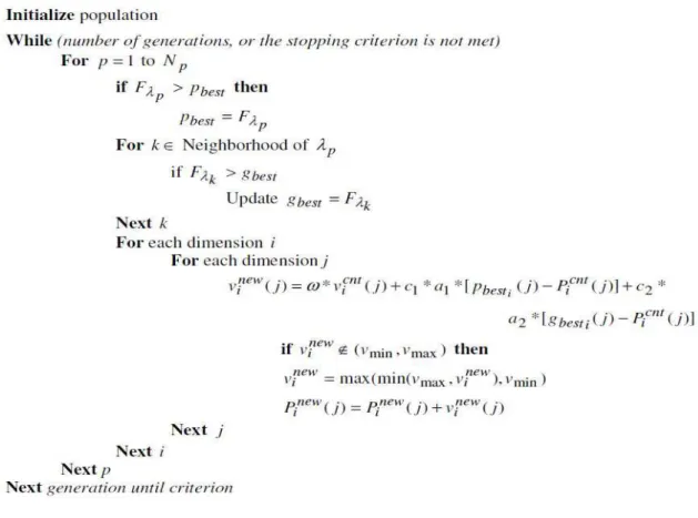
Fig. 1. Pseudo code for PSO method

In this pseudo code, v_icnt(j)stands for current velocity of the particle, v_inew(j)stands for new velocity of a particle, a₁and a₂ are arbitrary numbers in the interval[0,1], c₁and c₂ are acceleration constants (often chosen as 2.0) andωis inertia dampener which indicates the impact of the particle’s own experience on its next movement. Under the guidance of these two updating rules, the particles are attracted to move towards the best position found thus far. That is, the optimal solutions can be sought out due to this driving force. The corresponding optimum generation schedule is generated using the proposed PSO technique.

The major steps of PSO described in the pseudo code are discussed below:

a) Initialization

Initially, the particles of the swarm are selected randomly with the size ofN_p.Initialize a population of particles with random positions and velocities on N dimensions in the problem space. For each particle, evaluate the optimum fitness function in variables using eqn. (8). And compare the particles fitness evaluation with particlesp_best. If the current value is greater thanp_best, then setp_bestvalue equal to the current value and the pbest location equal to the current location in the dimensional space.

p N

i

j cnt

i j D ; j 1,2,...,N

P SC

FC F

p p

p  =

   

  

− +

+

=



=1 ) ( λ

λ

λ (8)

To calculate the pbest by using the fitness function, if the current value is greater than the previous pbest, then set the p_best value equal to the current value, and computeg_best, if the current value is better than g_best

then reset to the current particles.

b) Updating the Velocity

The velocity is updated by considering the current velocity of the particles and the best value obtained in fitness function among the particles in the swarm. The velocity of each particle is modified by using the updating rules mentioned in the pseudo code.

The value of the weighting factor ω is modified by the following eqn. for quick convergence.

iter iter * /

)

( _{max min max}

max ω ω

ω

Whereω_minand ω_maxare the minimum and maximum inertia weight factors respectively. iter is the current number of iterations and iter_max is the maximum number of iterations. The term ω < 1 is known as the “inertia weight”, and it is a friction factor chosen between 0 and 1 in order to determine to what extent the particle remains along its original course unaffected by the pull of the other two terms. It is very important to prevent oscillations around the optimal value.

c) Updating the Position

The velocity of each dimension has upper and lower limit,

v

_minand

v

_max and they are defined by the user. The velocity of such newly attained particle should be within the limits. Before proceeding further, this would be checked and corrected.

    < > = ) ( ) ( ; ) ( ) ( ) ( ; ) ( ) ( min min max max j v j v j v j v j v j v j v new i new i new

i (10)

Depend upon the newly obtained velocity vector; the position of each particle is updated by adding the updated velocity with current position of the individual in the swarm. The newly obtained particles are evaluated as mentioned earlier and so p_best for the new particles are determined.

With the concern of p_best and theg_best, new g_best is determined. Again by generating new particles, the same process is repeated until the process reaches the maximum iteration iter_max. Once the iteration reaches the iter_max, the process is terminated and so that a generation schedule of all the units with minimum cost is obtained which will meet the demand at the particular period. In the similar fashion, the optimum generating schedule for all the possible demand set is determined.

6.2 Determining Optimal Generation Schedule by EP

Evolutionary Programming (EP) is an optimization technique based on the natural generation. It involves random number generation at the initialization process. The generated random numbers represent the parameters responsible for the optimization of the fitness value. In addition, EP also involves fitness calculation, mutation and finally the new generation will be taken as a result of the selection. The basic steps of the original Evolutionary Programming Technique is as follows

1. Start with a random population of solutions.

2. For each of these, produce an offspring by mutation (produce a mutated form, which is its offspring). 3. The fitness of each population member is calculated.

4. Keep the best half of the population and remove the rest.

5. The best values of the first generation and their mutated offspring are combined as a new population. Using this new population as a starting point, repeat the process again until the solutions improve enough.

In the proposed method, there are two cases: the first case is finding the optimal generation schedule with minimum operating cost using only the current demand. But in the second case, we use both current and previous power demands to generate the optimal schedule with minimum operating cost and minimum CPU time. Both cases use the same processing steps, only the fitness calculation is different.

Case 1:

Step 1: Initialization of parent population

Initial population is one of the deciding factors for reaching the optimum; it should be carefully generated but always from the possible intervals. The initial population is composed by the

N

_p parent individuals. The elements of the parent are the randomly created permutation of the input variables of the generated units. Each element in a population is uniformly distributed with its feasible range. Each individual is taken as a pair of real valued vectors. } , , 2 , 1 { ) ,

(pi si ∀i∈  Np (11)

Where pi are the objective variables and determined by setting the jth component,

n j ; p p U ~

p_j ( _jmin, _jmax) =1,2,, whereU(pj_min,pj_max)denotes the uniform random variable

Evaluate the objective function, f(p) for each individual(p_i, s_i)∀i∈{1,2,,N_p}. The objective function

) (p

f is generated as

| |

min )

(p D D₁

f = _q− (12)

2 1|

| min )

(p D_qi D_i

f = − i=1,2 (13)

Step 2: Fitness calculation

Putative solutions to the target problem are evaluated using "Fitness functions", otherwise known as "Objective functions". The fitness of all individuals in a population is calculated to determine the degree of optimality. The fitness function for each parent (p_i, s_i)∀i∈{1,2,N_p}of the initial population is computed as

)

( _{q i}

i D D

F = − i=1,2,,N_p (14)

Here D_q is the query demand and Di is the demand in the optimum generation schedule already obtained

by PSO.

Step 3: Mutation

Mutation is the random occasional alteration of the information contained in the individual. It is performed on each element by adding a normally distributed random number with mean few and standard deviation. Create the offspring population p 'i using the mutation process.

) , 0

( 2

, N σ

p

p'_i = _{i j}+ (15)

      − = max min max

2 _{( )}

F F p

p_{j j} i

β

σ (16)

p

N

i=1,2 and j=1,2N_p

Where the p_i,j denotes the jth element of ith individual and N(0,σ2) is a Gaussian random variable with mean and standard deviation. F_maxis the maximum fitness value of old generation. p_jmax and p_jmin are the maximum and minimum limits of the jth element. β is the mutation scale which is given as 0 ≤β≤ 1. Add the Gaussian random variable N(0,σ2) to the entire state variable of p_i to getp'_i. Here 0 is a mean and σ2is a standard deviation. The fitness value corresponding to each offspring obtained from mutation is computed by running a load flow with the unit generations of each offspring and using equation.

Step 4: Competition and Selection

Each individual in the combined population of N_p parent trial vectors and their corresponding N_p

offspring has to compete with

r

number of individuals, randomly chosen from the combined population, to have a chance to survive to the next generation. The value of

r

may be equal to the population size of the

parent population. Select the N_p individuals from the total 2N_p individuals of both p_i and p'_i using the following rule

Evaluate each trail vector by



= = p N x x pi W W 1

where i=1,2,,2N_psuch that

 

 < + <

= otherwise ; f f f 0 if ;

W_x t t i

0 1 ) ( 1 (17)

where Wpiis a weight value assigned to each individual. ft is the fitness of the tth competitor randomly

 

 + >

=

otherwise ;

f f f if

W_x t t i

0

5 . 0 ) /( ; 1

(18)

The weight assignment is found to yield the proper selection and good convergence. When all the 2N_p

individuals are obtain their weights, they are ranked in descending order and the first Np individuals are

selected as parents along with their fitness values with their next generation.

Step 5: Convergence

During initialization the maximum number of generation is fixed and it is checked for convergence. If the convergence condition is not met, the mutation and competition process is run again. The maximum generation number is used for convergence condition. The process is terminated if the maximum number of generations are reached otherwise the above procedure is repeated from step (2 - 4). Generations are also repeated until

f

f_avg / )≥δ

( _max (19)

Here f_avg is the average fitness value and f_maxis the maximum fitness value and

δ

should be very close to 1, which represents the degree of satisfaction.

Case 2:

In case 2, all the processing steps are same as case 1 and only the fitness calculation is different. For case 2, both current and previous demands are used to optimize the schedule. So the fitness can be calculated as

2

) ' (

) '

( 2 2

2

1 i q i

q i

D D D

D

F = − + − i=1,2 (20)

Where, Dq₁ and Dq2are the query demand and Di' are the offspring created during the mutation. These steps

are repeated until the optimum fitness is reached. Eventually, by using both case 1 and case 2, the commitments of units in an optimal manner are obtained so as to fulfill the demand at the particular period by satisfying the mentioned constraints.

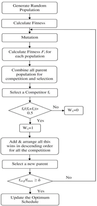
Fig .2. Steps involved in EP to determine the optimal generation schedule

7. Results and Discussion

Table 1. Operation data of IEEE-30 bus utility system

Unit A, US$ B, $/MW _{C, $/MW2} PSi min, MW

PSi max, MW

1 77.84 6.42 0.003 12 50 250

2 95.14 5.94 0.005 45 75 250

3 235.97 7.46 0.004 13 75 250

4 276.54 8.35 0.002 54 145 310

5 216.54 8.15 0.002 72 150 310

6 312.76 9.54 0.002 15 150 320

7 262.63 8.94 0.002 56 160 350

8 237.21 7.42 0.003 32 167 350

9 327.32 6.77 0.004 76 180 380

10 337.42 7.74 0.003 78 180 412

11 213.43 5.56 0.001 25 188 412

12 123.56 6.67 0.003 21 188 125

13 129.34 6.43 0.005 12 75 125

14 145.56 5.56 0.008 16 75 150

15 178.34 5.89 0.007 76 80 150

16 234.89 4.32 0.007 21 80 220

17 211.78 3.67 0.006 12 85 220

18 206.23 7.45 0.003 21 85 230

19 206.75 6.56 0.006 78 90 230

20 145.34 4.43 0.009 12 90 250

21 123.56 5.56 0.007 15 95 250

22 119.34 5.12 0.005 43 95 250

23 112.51 8.43 0.003 89 90 300

24 178.67 7.48 0.005 41 110 300

25 150.55 5.89 0.006 98 110 320

26 150.21 5.12 0.001 89 110 320

27 150.54 9.21 0.005 67 110 320

28 145.55 5.87 0.003 61 110 330

29 178.21 9.65 0.005 60 120 330

30 176.78 8.34 0.004 52 120 330

Table 2: Optimal generation schedule for IEEE-30 bus utility system satisfying 24 hours demand along with its Total Operating Cost.

Tim

e 1 2 3 4 5 6 7 8 9 10 11 12 13 14 15 16 17 18 19 20 21 22 23 24

T

o

ta

l O

p

er

at

in

g C

o

st

(p.

u

)

P

owe

r Dem

a

nd

(MW)4560 4570 4560 4570 4580 4590 4600 4650 4660 4690 4800 4850 4900 4700 4800 4850 4860 4870 4900 4950 4960 4970 4700 4610

Unit s

0.989 6

1 250 184 184 146 148 184 189 0

206.

5 109 199 203.5 255.5 0 223. 5

112.

5 0 194 0 0 0 0 194 189.5

2 0 0 0 0 0 0 0 0 0 0 0 0 0 0 0 0 0 84 0 0 0 0 84 0

3 0 0 0 0 0 0 0 0 0 0 0 0 0 0 0 0 0 0 0 0 0 0 0 0

4 310 310 310 310 310 310 310 180 310 310 310 310 310 272 310 310 226 310 238 223 225.5 241.

5 310 310

5 0 276 286 310 310 286 0 9.5

303.

5 310 310 306.5 310 180 0 310 180 282 180 180 180 180 282 299.5

6 320 0 0 320 0 0 320 412 320 320 320 320 320 380 320 320 380 320 380 380 380 380 320 320

7 340 350 350 350 350 350 350 412 350 350 350 350 350 380 330 350 380 350 380 380 380 380 350 350 8 340 350 350 350 350 350 301 412 350 350 350 350 350 380 330 350 380 350 380 380 380 380 350 291 9 340 360 360 380 360 360 380 412 380 370 380 380 360 266 330 360 348 380 334 354 349 337 380 380 10 340 360 360 390 360 360 410 254 410 370 390 410 360 380 330 360 380 390 380 380 380 380 390 410 11 340 360 360 390 360 360 410 412 410 370 390 410 360 380 330 360 380 390 380 380 380 380 390 410

12 0 0 0 0 0 0 0 0 0 0 0 0 0 0 0 0 0 0 0 0 0 0 0 0

14 0 0 0 0 0 0 0 0 0 0 0 0 0 0 0 0 0 0 0 0 0 0 0 0

15 0 0 0 0 0 0 0 0 0 0 0 0 0 0 0 0 0 0 0 0 0 0 0 0

16 0 0 0 0 0 0 0 0 0 0 0 0 0 0 0 0 0 0 0 0 0 0 0 0

17 0 0 0 0 0 0 0 0 0 0 0 0 0 0 0 0 0 0 0 0 0 0 0 0

18 0 0 0 0 0 0 0 0 0 0 0 0 0 0 0 0 0 0 0 0 0 0 0 0

19 0 0 0 0 0 0 0 0 0 0 0 0 0 0 0 0 0 0 0 0 0 0 0 0

20 0 0 0 0 0 0 0 0 0 0 0 0 0 0 0 0 0 0 0 0 0 0 0 0

21 0 0 0 0 0 0 0 0 0 0 0 0 0 0 0 0 0 0 0 0 0 0 0 0

22 0 0 0 0 0 0 0 0 0 0 0 0 0 0 0 0 0 0 0 0 0 0 0 0

23 0 0 0 284 262 0 0 0 0 300 291 0 294.5 92 246.5300 46 0 58 43 45.5 61.5 0 0

24 0 0 0 0 0 0 0 0 0 0 0 0 0 0 0 217.50 0 0 0 0 0 0 0

25 320 320 320 320 320 320 320 412 320 320 320 320 320 380 320 320 380 320 380 380 380 380 320 320 26 320 320 320 320 320 320 320 379 320 320 320 320 0 380 320 320 380 320 380 380 380 380 320 320

27 320 320 320 320 320 320 320 189.5 320 320 320 320 320 380 320 0 380 320 380 380 380 380 320 320

28 330 330 330 0 330 330 330 412 330 201 0 330 330 380 330 330 380 330 380 380 380 380 330 330 29 330 330 330 330 330 330 330 412 330 330 330 330 330 380 330 330 380 330 380 380 380 380 330 330 30 330 330 330 330 330 330 330 412 330 330 330 330 330 380 330 330 380 330 380 380 380 380 330 330

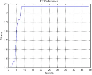
The demand for 24 hour time horizon is just a simulation and not the actual demand which the units satisfy practically. Evolutionary Programming (EP) is used to obtain an optimum generation schedule for each period and the total operating cost for the whole 24 hour period. The optimal generation schedule for a particular demand is determined by the contribution of PSO-EP. Fig 3 depicts the performance of EP for a particular demand.

Fig .3. Convergence characteristics of Evolutionary Programming approach

PSO generates an optimal unit commitment with minimum cost for a given demand. Fig 3, illustrates the improvement in fitness with reference to minimum cost operation of the commitment units. The graph is obtained by solving the power demand of 4700 MW by IEEE 30 bus system. The fitness value is optimized in all iterations. After a certain number of iterations, the fitness value does not change, which means that the optimum fitness value is converged. For the evaluation of performance, we have solved the UCP by using PSO and EP and the computational time taken by the proposed hybrid approach has been compared with that of the previous hybrid approach PSO-ANN. The comparison result between the proposed hybrid approach and the previous PSO-ANN is tabulated in Table 3.

Table 3. Comparison between the Proposed PSO-EP approach and the PSO-ANN approach in solving the UCP by means of CPU time

CPU time (sec) Proposed PSO EP Hybrid

approach IEEE-30 bus utility System 0.141552

Proposed PSO ANN

The proposed PSO-EP hybrid approach takes considerably less CPU time for generating the optimal schedule of IEEE-30 bus utility system compared with the previous hybrid approach which is based on PSO-ANN. Hence it can be confirmed that the proposed hybrid approach is capable of generating effective optimum generation schedules in less time.

8. Conclusion

The proposed hybrid approach which uses PSO and EP exhibits good performance in solving the UCP by recognizing the optimal generation schedule. In the proposed method, mutation, competition and selection are the essential processes simulated in the procedure. The approach has been tested for the IEEE-30 bus utility system with consideration to the most significant load balance and spinning reserve constraints. Prior to the system test, we have different possible combinations of the demand set and its corresponding optimal schedule. For the test demand set, which consists of demand for a 24 hour period, the hybrid approach effectively yields optimal generation schedule for all the periods. Moreover, we have compared the test results of the proposed hybrid approach with the discrete performance of the previous hybrid approach PSO-ANN. For UCP more efficient solutions are produced by the hybridized PSO-EP method. Hence, it could be concluded that the approach gives optimal commitment schedule of units for any given demand that satisfies the defined constraints as well as the demand with minimum cost.

References

[1] S. Senthil Kumar and V. Palanisamy, "A Hybrid Fuzzy Dynamic Programming Approach to Unit Commitment", Journal of the Institution of Engineers (India) Electrical Engineering Division, Vol. 88, No. 4, 2008.

[2] Christober C. Asir Rajan, "Genetic Algorithm Based TABU Search Method for Solving Unit Commitment Problem with Cooling Banking Constraint", Journal of Electrical Engineering, Vol. 60, No. 2, pp. 69-78, 2009.

[3] U. Basaran Filik and M. Kurban, "Fuzzy Logic Unit Commitment based on Load Forecasting using ANN and Hybrid Method", International Journal of Power, Energy and Artificial Intelligence, Vol. 2, No.1, pp. 78- 83, March 2009. [4] Jorge Pereira, Ana Vienna, Bogdan G. Lucus and Manuel Matos, "Constrained Unit Commitment and Dispatch

Optimization", 19th Mini-EURO Conference on Operation Research Models and Methods in the Energy Sector, Coimbra, Portugal, 2006.

[5] R. Nayak and J.D. Sharma, "A Hybrid Neural Network and Simulated Annealing Approach to the Unit Commitment Problem", Computers and Electrical Engineering, Vol. 26, No. 6, pp. 461-477, 2000.

[6] Ali Keles, A. Şima Etaner-Uyar and Belgin Türkay, "A Differential Evolution Approach for the Unit Commitment Problem", In ELECO 2007: 5th International Conference on Electrical and Electronics Engineering, pp. 132-136, 2007. [7] Kris R. Voorspools and William D. D’haeseleer, "Long Term Unit Commitment Optimization for Large Power

Systems; Unit Decommitment versus Advanced Priority Listing", Applied Energy, Vol. 76, No. 1-3, pp. 157-167, 2003. [8] Kaveh Abookazemi, Mohd Wazir Mustafa and Hussein Ahmad, "Structured Genetic Algorithm Technique for Unit

Commitment Problem", International Journal of Recent Trends in Engineering, Vol. 1, No.3, May 2009.

[9] S. Prabhakar karthikeyan, K.Palanisamy, I. Jacob Raglend and D. P. Kothari, "Security Constrained UCP with Operational and Power Flow Constraints", International Journal of Recent Trends in Engineering, Vol. 1, No. 3, May 2009.

[10]Ali Keles, "Binary Differential Evolution for the Unit Commitment Problem", In Proceedings of the 2007 GECCO conference companion on Genetic and evolutionary computation, pp. 2765-2768, 2007.

[11]V. Senthil Kumar and M.R. Mohan, "Genetic Algorithm with Improved Lambda- Iteration Technique to solve the Unit Commitment Problem", In proc. of Intl. Journal on Electrical and Power Engineering, Vol. 2, No. 2, pp. 85- 91, 2008. [12]A. Sima Uyar and Belgin Turkay, "Evolutionary Algorithms for the Unit Commitment Problem", In proc. of Turkish

Journal on Electrical Engineering, vol. 16, no. 3, pp. 239- 255, 2008.

[13]S.Chitra Selvi, R.P.Kumudini Devi and C.Christober Asir Rajan, "Hybrid Evolutionary Programming Approach to Multi-Area Unit Commitment with Import and Export Constraints", In proc. of International Journal on Recent Trends in Engineering, Vol. 1, No. 3, May 2009.

[14]Antonio Frangioni and Claudio Gentile, "Solving Nonlinear Single-Unit Commitment Problems with Ramping Constraints", Operations Research, vol. 54, no. 4, pp. 767- 775, July- August 2006, Doi: 10.1287/opre.1060.0309. [15]Xiaohong Guan, Sangang Guo, and Qiaozhu Zha, "The Conditions for Obtaining Feasible Solutions to

Security-Constrained Unit Commitment Problems", IEEE Transactions on Power Systems, Vol. 20, No.4, November 2005. [16]Erlon C. Finardi, Edson L. Da Silva And Claudia Sagastizábal, "Solving the unit commitment problem of hydropower

plants via Lagrangian Relaxation and Sequential Quadratic Programming", Computational and Applied Mathematics, Vol. 24, no. 3, pp. 317- 341, 2005.

[18]Abdul Rahman Minhat, Ismail Musirin and Muhammad Murtadha Othman, "Evolutionary Programming based Technique for secure Operating Point Identification in Static Voltage Stability Assessment", Journal of Artificial Intelligence, Vol. 1 pp.12-20, 2008.

[19]Ling-Feng Hsieh, Chao-Jung Huang and Chien-Lin Huang, "Applying Particle Swarm Optimization To Schedule Order Picking Routes In A Distribution Center", Asian Journal Of Management And Humanity Sciences, Vol. 1, No. 4, Pp. 558-576, 2007.

[20]Rabab M. Ramadan and Rehab F. Abdel-Kader, "Face Recognition Using Particle Swarm Optimization-Based Selected Features", International Journal of Signal Processing, Image Processing and Pattern Recognition, Vol. 2, No. 2, 2009. [21]W. T. Li, X. W. Shi and Y. Q. Hei, "An Improved Particle Swarm Optimization Algorithm For Pattern Synthesis Of

Phased Arrays", Progress In Electromagnetics Research, pp. 319–332, 2008.

[22]Ching-Yi Chen, Hsuan-Ming Feng and Fun Ye, "Hybrid Recursive Particle Swarm Optimization Learning Algorithm in the Design Of Radial Basis Function Networks," Journal Of Marine Science And Technology, Vol. 15, No. 1, pp. 31-40, 2007.

[23]D. Nagesh Kumar and M. Janga Reddy, "Multipurpose Reservoir Operation Using Particle Swarm Optimization", Journal of Water Resources Planning and Management, Vol. 133, No. 3, pp. 192-201, 2007.

[24]Faten Ben Arfia, Mohamed Ben Messaoud, Mohamed Abid, "Nonlinear adaptive filters based on Particle Swarm Optimization", Leonardo Journal of Sciences, No. 14, pp. 244-251, 2009.

[25]Qi Kang, Lei Wang and Qi-di Wu, "Research on Fuzzy Adaptive Optimization Strategy of Particle Swarm Algorithm", International Journal of Information Technology, Vol.12, No.3, pp.65-77, 2006.

[26]Rehab F. Abdel-Kader, "Particle Swarm Optimization for Constrained Instruction Scheduling", VLSI Design, Vol. 2008, No. 4, pp. 1-7, 2009.

[27]R.Karthi, S.Arumugam and K. Rameshkumar, "Comparative Evaluation of Particle Swarm Optimization Algorithms for Data Clustering using real world data sets", International Journal of Computer Science and Network Security, Vol. 8, No.1, 2008.

[28]A. J. Wood and B. F. Woolenberg, “Power Generation and Control”, II edition, New York: Wiley, 1996.

[29]K.A. Juste, H. Kita, E. Tanaka, J. Hasegawa,” An Evolutionary Programming Solution to the Unit Commitment Problem”, IEEE Transaction on Power Systems, Vol. 14, No. 4, pp. 1452-1459, 1999.

[30]H.T. Yang, P.C. Yang, and C.L. Huang, ”Evolutionary Programming Based Economic Dispatch for Units with Non-smooth Fuel Cost Functions”, IEEE Transaction on Power Systems, Vol. 11, No. 1, pp. 112-118, 1996.

[31]C. Christober Asir Rajan and M. R. Mohan, "An Evolutionary Programming-Based Tabu Search Method For Solving The Unit Commitment Problem", IEEE Transactions On Power Systems, Vol. 19, No. 1, February 2004.

[32]Nidul Sinha, Bipul Syam Purkayastha and Biswajit Purkayastha,"Hybrid Pso/ Self-Adaptive Evolutionary Programs For Economic Dispatch With Non smooth Cost Function", International Journal of Recent Trends in Engineering, Vol. 1, No. 3,pp.195-200, May 2009.

[33]B Saravanan C. Rani, S.Prabhakar Karthikeyan, I. Jacob Raglend and D.P. Kothari, “Profit based Unit Commitment Problem with Fuel and Emission Constraints using LR-EP approach”, Emerging Journal of Engineering Science and Technology, Vol. 3, No.5, pp. 53-66, August 2009.

[34]Yuan-Yin Hsu, Chung-Ching Su, Chih-Chien Liang, Chia-Jen Lin and Chiang-Tsung Huang, "Dynamic security constrained multi-area unit commitment", IEEE Transactions on Power Systems, Vol. 6, Issue 3, pp. 1049-1055, August 2002.

[35]Xin Yao, Yong Liu, and Guangming Lin, "Evolutionary Programming Made Faster", IEEE Transactions On Evolutionary Computation, Vol. 3, No. 2, July 1999.

[36]N Sinha, R Chakravarthi, and P K Chattopadhyay, “Improved Fast Evolutionary Program for Economic Load Dispatch with Non-Smooth Cost Curves”, Institute Of Engineers Journal-EL, Vol. 84, pp. 110-114, September 2004.

[37]Grzegorz Dudek, "Adaptive simulated annealing schedule to the Unit Commitment Problem”, Electric Power Systems Research, Vol. 80, No. 4, pp. 465-472, April 2010.

R Lal Raja Singh, born on 1979 and received his BE Electrical and Electronics degree from university of Madras, Chennai and M.Tech degree in Power Electronics and Drives degree from Uttar Pradesh Technical University, Lucknow, India in 2001 and 2003respectively. He is currently pursuing the Ph.D degree in Electrical Engineering at Sathyabama University, Chennai, India. Currently, he is an Assistant Professor in the Electrical and Electronics Engineering Department at Marthandam College of Engineering and Technology, Kuttakuzhi, India.