1
A Novel MILP Model to Solve Killer Samurai
Sudoku Puzzles
Jose B. Fonseca
Department of Electrical Engineering and Computer Science Faculty of Sciences and Technology
New University of Lisbon
Monte de Caparica, 2829-516 Caparica, Portugal Email:[email protected]
Abstract—A Killer Samurai Sudoku puzzle is a NP-Hard problem and very nonlinear since it implies the comparison of areas or cages sums with their desired values, and humans have a lot of difficulty to solve these puzzles. On the contrary our mixed integer linear programming (MILP) model, using the Cplex solver, solves easy puzzles in few seconds and hard puzzles in few minutes. We begin to explain why humans have such a great difficulty to solve Killer Samurai Sudoku puzzles, even for low level of difficulty ones, taking into account the cognitive limitations as the very small working memory of 7-8 symbols. Then we briefly review our previous work where we describe linearization techniques that allow solving any nonlinear problem with a linear MILP model [1]. Next we describe the sets of constraints that define a Killer Sudoku puzzle and the definition of the objective variable and the implementation of the solution of a Killer Samurai Sudoku puzzle as a minimization problem formulated as a MILP model and implemented with the GAMS software. Finally we present the solutions of a hard Killer Samurai Sudoku puzzles with our MILP model using the Cplex solver.
Keywords–Intelligence; OR; AI; MILP; Puzzles
I. INTRODUCTION
The first problems solved by Artificial Intelligence (AI) and Operations Research (OR) were toy problems, games and more recently puzzles. In the eighties there were annual tournaments of chess computer programs and Kasparov was even defeated by one of these chess programs. More recently Sudoku appeared in Japan and then Kakuro and Killer Sudoku puzzles that were rapidly disseminated through the rest of the world. More recently arose the Killer Samurai Sudoku puzzles that consist of five Killer Sudoku puzzles with the fifth puzzle overlapping over the remaining four puzzles. As an alternative approach to AI, in this work we formulate the Killer Sudoku puzzle problem solution as an optimization problem with constraints in the framework of a Mixed Integer Linear Program (MILP) model and then solve it using the Cplex solver with the GAMS software. A Killer Sudoku puzzle consists of a matrix of dimension 9x9 where each line and column must be a permutation of integers between 1 and 9, each sub-matrix 3x3 must be a permutation of these numbers and there are a set of colour areas or cages that must have a predefined sum. The runtimes of the solution of a black belt Killer Sudoku puzzle [1] using our MILP model were very
small, just some few seconds. To our knowledge this is the first proposal to solve a Killer Sudoku puzzle. Nevertheless in a previous work [1] we solved Kakuro puzzles with a MILP model and the runtimes showed to be much lower than then the runtimes of previous proposals [2-3].
II. WHAT ISMATHEMATICALPROGRAMMING? WHAT IS AMILP MODEL?
A mathematical program is a set of inequalities and equalities defined in terms of the model variables, one of them defining the objective variable that must be maximized or minimized. In a linear model all constraints are linear and it cannot be applied any nonlinear operation over a model variable neither exists the product between two model variables. A mixed integer linear program (MILP) is a linear model with integer, binary and continuous variables. In this work we used the GAMS modeling language to formulate the puzzle as an optimization problem and solve it with an algorithm, the Cplex solver. For example the simplified code that implements a MILP model to obtain the maximum and minimum of a given array would be:
sets i /1*20/; parameter a_p(i); a_p(i)=ord(i)-10;
variable a(i), minimum, maximum, obj; **CONSTRAINTS**
**set the array elements: set_a(i).. a(i)=e=a_p(i);
**the minimum is less or equal to all elements of a(i): calc_min(i).. minimum =l= a(i);
**the maximum is greater or equal to all elements of a(i): calc_max(i).. maximum =g= a(i);
**to prevent trivial solutions we must maximize the minimum and minimize the maximum: calc_obj.. obj=e= minimum - maximum;
Model MaxMin /all/;
Solve MaxMin using MIP maximizing obj; display a.l, obj.l, maximum.l, minimum.l;
The constraint calc max(i) implements the setof inequali-ties (1).
∀i, maximum ≥ a(i) (1)
GAMS Rev 229 WIN-VIS 22.9.2 x86/MS Windows 03/09/16 17:01:32 Page 6 G e n e r a l A l g e b r a i c M o d e l i n g S y s t e m
E x e c u t i o n ---- 26 VARIABLE a.L
1 -9.000, 2 -8.000, 3 -7.000, 4 -6.000, 5 -5.000, 6 -4.000 7 -3.000, 8 -2.000, 9 -1.000, 11 1.000, 12 2.000, 13 3.000 14 4.000, 15 5.000, 16 6.000, 17 7.000, 18 8.000, 19 9.000 20 10.000
---- 26 VARIABLE obj.L = -19.000 VARIABLE maximum.L = 10.000 VARIABLE minimum.L = -9.000
EXECUTION TIME = 0.078 SECONDS 3 Mb WIN229-229 Dec 1, 2008
III. DESCRIPTION OF OURMILP MODEL TOSOLVE
KILLERSUDOKUPUZZLES
The main element of our Killer Sudoku MILP model is an indexed binary variable with three indexes that defines the 9x9 matrix which must be filled with integer numbers between 1..9. The first and second indexes represent the line and column of the matrix element, respectively, and the third index represents the value of the matrix element, i.e. there is only value of the third index for which the binary variable is one and all the remaining are zero for a given line and column. This way the order of the last index of this indexed binary variable is translated into the value of the Killer Sudoku matrix element. This is the main idea to linearize this so nonlinear problem. With this approach the constraints, like the all different constraints, are very elegant and simple and the runtimes are very small. First we must impose that each matrix element has only one value, which seems obvious but must be declared since the value of the matrix element is expressed by the order of the third index of the indexed binary variable a bin(l,c,v),landcbeing the line and column of the matrix element and the order of index vits value. This condition is expressed by the set of equality constraints (2).
∀l, c,X
v
a bin(l, c, v) = 1 (2)
The set of constraints (1) can be implementated with GAMS syntax as:
only one(l,c).. sum(v,a bin(l,c,v))=e=1;
Next we must impose that there are no repetitions in each line l, the all different constraint, i.e. for each pair of values (l, v) summing the binary indexed variable a bin(l,c,v) over all columns c, this sum must be equal to 1, since in a Killer Sudoku puzzle each line is a permutation of integer numbers between 1 and 9. This set of logical conditions or constraints is expressed by the set of nonlinear constraints (3).
∀l, v,X
c
a bin(l, c, v) = 1 (3)
The set of constraits (2) can be implementated with GAMS syntax as:
all different line(l,v).. sum(c,a bin(l,c,v))=e=1;
In other words (3) ensures that each line is a permutation of integer numbers between 1 and 9. And there must not exist repetitions in each column, what is expressed by the similar set of logical conditions or constraints (4), the all different constraint for each column c.
∀c, v,X
l
a bin(l, c, v) = 1 (4)
The set of constraits (4) can be implementated with GAMS syntax as:
all different column(c,v).. sum(l,a bin(l,c,v))=e=1;
Next we impose that each sub-matrix 3x3 must be a per-mutation of integers between 1 and 9. To express this set of logical conditions we created an auxiliary indexed parameter, square(l1,c1,l,c), which is initialized by the set of equations (5),
∀l1, c1, l, c, (5)
square(l1, c1, l, c) = (l≥((l1−1)Order+ 1))
(l≤((l1−1)Order) +Order)
(c≥((c1−1)Order+Order)) .
In (5) the multiplication of inequalities must be interpreted as the logical AND of the logical values of the inequalities. The scalar Orderdefines the dimension of the Killer Sudoku puzzle sub-matrix and for the classical Killer Sudoku puzzles Order=3. Then the set of logical conditions or constraints that impose that each sub-matrix Order x Order must have no repetitions is expressed by the set of equations (6).
∀l1, c1, v1,
X
(l,c): square(l1,c1,l,c)=1
a bin(l, c, v1) = 1 (6)
Equation (6) can be written using GAMS syntax as:
all different square(l1,c1,v1).. sum((l,c)$(square(l1,c1,l,c)), a bin(l,c,v1)) =e=1;
∀col, (7)
X
v,(l,c):colour bin(col,l,c)=1
v a bin(l, c, v) =sum colour(col)
Equation (7) can be written using GAMS syntax as:
sum colour segment(col).. sum((l,c,v1)$(colour bin(col,l,c) ),ord(v1)*a bin(l,c,v1)) =e=sum colour(col);
Finally to prevent trivial solutions with all values of a bin(i,j,v)=1 we must minimize the objective variable defined as the number of matrix elements, which is expressed by equation (8).
obj=X
i,j,v
a bin(i, j, v) (8)
Equation (8) can be implemented in GAMS code as:
calc obj..obj=e=sum((i,j,v),a bin(i,j,v));
IV. SOLUTION OFTWOBlack BeltKILLERSUDOKU
PUZZLES WITH OURMILP MODEL
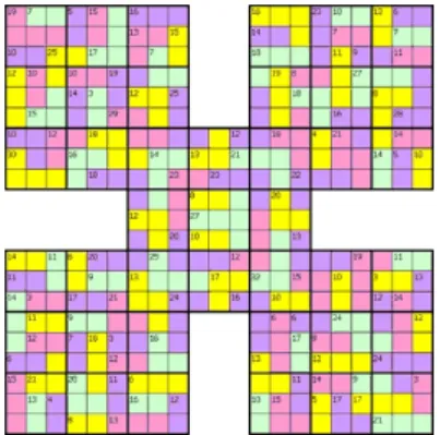
In figure 1 we show a hard Killer Sudoku puzzle taken from [2] that we solved with our MILP model in just few seconds in a PC with 2GHz clock and in appendix 2 we show the output of the GAMS software code that corresponds to the first solution. Note that in this hard Killer Sudoku puzzle each different area of matrix elements whose sum must be equal to the number printed in the region. Moreover these puzzle has two regions with four elements which contribute to the combinatorial explosion in the ways the matrix elements may be filled.
Figure 1: Killer Sudoku puzzle solved by our MILP model
V. CONCLUSIONS ANDFUTUREWORK
We showed that our MILP model to solve Killer Sudoku puzzles is very efficient and elegant. In a near future we plan to expand our MILP model to solve variants of Killer Sudoku like Killer Sudoku Greater Than and then adapt them to develop a MILP model to make production planning based on a MILP model and the Cplex solver. In appendix 1 we show the GAMS code that implements our MILP model with some instructions of parameter definition omitted. In a near future we plan to adapt our MILP model to solve a variation of Killer Sudoku puzzles, the Killer Sudoku Greater Than puzzles where there are also logical conditions between cages sums.
REFERENCES
[1] J. Barahona da Fonseca, Solving Any Nonlinear Problem with a MILP Model. Proceedings of Escape-19 Conference, 2009.
[2] djape, Killer Sudoku and other puzzle variants, 2010.
[3] R. P. Davies, An Investigation into the Solution to, and Evaluation of, Kakuro Puzzles, MSc thesis, University of Glamorgan, 2009.
[4] H. Simonis, Kakuro as a Constraint Problem, in Proceedings of Modref Conference, 2008.
APPENDIX
GAMS Implementation of our Novel MILP Model to Solve Any Killer Sudoku Puzzle
In the following GAMS code the names of constraints always finish with .. .
sets l /1*21/; alias(c, l); set v1 /1*9/; alias(v, v1); set c1 /1*3/; alias(l1, c1); set col /1*129/;
*121-*positive variable a(l,c); binary variable a_bin(l,c, v1); scalar Order /3/;
Parameter square(l1,c1,l,c), square2(l1,c1,l,c), square3(l1,c1,l,c), square4(l1,c1,l,c), square5(l1,c1,l,c), cor_bin(col, l, c), soma_cor(col);
square(l1,c1,l,c)=(ord(l) ge ((ord(l1)-1)*Order+1) )*(ord(l) le ((ord(l1)-1)*Order+Order)) *(ord(c) ge ((ord(c1)-1)*Order+1))*(ord(c) le ((ord(c1)-1)*Order+Order));
square2(l1,c1,l,c)=(ord(l) ge ((ord(l1)-1)*Order+1) )*(ord(l) le ((ord(l1)-1)*Order+Order)) *(ord(c) ge (12+(ord(c1)-1)*Order+1))*(ord(c) le (12+(ord(c1)-1)*Order+Order));
square3(l1,c1,l,c)=(ord(l) ge (12+(ord(l1)-1)*Order+1) )*(ord(l) le (12+(ord(l1)-1) *Order+Order))
*(ord(c) ge ((ord(c1)-1)*Order+1))*(ord(c) le ((ord(c1)-1)*Order+Order)); square4(l1,c1,l,c)=(ord(l) ge (12+(ord(l1)-1)*Order+1) )*(ord(l) le (12+(ord(l1)-1)* Order+Order))
*(ord(c) ge (12+(ord(c1)-1)*Order+1))*(ord(c) le (12+(ord(c1)-1)*Order+Order)); square5(l1,c1,l,c)=(ord(l) ge (6+(ord(l1)-1)*Order+1) )*(ord(l) le (6+(ord(l1)-1) *Order+Order))
*(ord(c) ge (6+(ord(c1)-1)*Order+1))*(ord(c) le (6+(ord(c1)-1)*Order+Order)); *Next we define the cages of the first puzzle
soma_cor(’1’)=6;
************************************* cor_bin(’2’, ’1’, ’2’)=1;
cor_bin(’2’, ’2’, ’2’)=1; cor_bin(’2’, ’3’, ’2’)=1; cor_bin(’2’, ’3’, ’1’)=1; soma_cor(’2’)=23;
************************************* cor_bin(’3’, ’1’, ’3’)=1;
cor_bin(’3’, ’1’, ’4’)=1; soma_cor(’3’)=13;
************************************* cor_bin(’4’, ’1’, ’5’)=1;
cor_bin(’4’, ’1’, ’6’)=1; soma_cor(’4’)= 17;
************************************* cor_bin(’5’, ’1’, ’7’)=1;
cor_bin(’5’, ’1’, ’8’)=1; cor_bin(’5’, ’1’, ’9’)=1; soma_cor(’5’)=8;
************************************* cor_bin(’6’, ’2’, ’3’)=1;
cor_bin(’6’, ’2’, ’4’)=1; cor_bin(’6’, ’2’, ’5’)=1; cor_bin(’6’, ’2’, ’6’)=1; soma_cor(’6’)=15;
* snip! some instructions omitted variable obj;
* CONSTRAINTS:
*only_one(l,c).. sum(v1, a_bin(l,c,v1))=e=1;
only_one(l,c)$( (ord(l) ge 1) * (ord(l) le 9) * (ord(c) le 9) * (ord(c) ge 1) ).. sum(v1, a_bin(l,c,v1))=e=1;
only_one2(l,c)$( (ord(l) ge 1) * (ord(l) le 9) * (ord(c) le 21) * (ord(c) ge 13) ) .. sum(v1, a_bin(l,c,v1))=e=1;
only_one3(l,c)$( (ord(l) ge 7) * (ord(l) le 15) * (ord(c) le 15) * (ord(c) ge 7) ).. sum(v1, a_bin(l,c,v1))=e=1;
only_one4(l,c)$( (ord(l) ge 13) * (ord(l) le 21) * (ord(c) le 9) * (ord(c) ge 1) ).. sum(v1, a_bin(l,c,v1))=e=1;
only_one5(l,c)$( (ord(l) ge 13) * (ord(l) le 21) * (ord(c) le 21) * (ord(c) ge 13) ).. sum(v1, a_bin(l,c,v1))=e=1;
all_different_line(l,v1)$( ord(l) le 9).. sum(c$(ord(c) le 9), a_bin(l,c,v1))=e=1; all_different_line2(l,v1)$( ord(l) le 9)..
sum(c$( (ord(c) le 21) * (ord(c) ge 13) ), a_bin(l,c,v1))=e=1; all_different_line3(l,v1)$( (ord(l) le 15) * (ord(l) ge 7) )..
sum(c$( (ord(c) le 15) * (ord(c) ge 7) ), a_bin(l,c,v1))=e=1; all_different_line4(l,v1)$( (ord(l) le 21) * (ord(l) ge 13) )..
sum(c$( (ord(c) le 9) * (ord(c) ge 1) ), a_bin(l,c,v1))=e=1; all_different_line5(l,v1)$( (ord(l) le 21) * (ord(l) ge 13) )..
sum(c$( (ord(c) le 21) * (ord(c) ge 13) ), a_bin(l,c,v1))=e=1;
all_different_column(c,v1)$(ord(c) le 9).. sum((l)$(ord(l) le 9), a_bin(l,c,v1))=e=1; all_different_column2(c,v1)$( (ord(c) le 21) * (ord(c) ge 13) )..
sum((l)$( ord(l) le 9 ), a_bin(l,c,v1))=e=1;
all_different_column3(c,v1)$( (ord(c) le 15) * (ord(c) ge 7) ).. sum((l)$( (ord(l) le 15) * (ord(l) ge 7) ), a_bin(l,c,v1))=e=1; all_different_column4(c,v1)$( (ord(c) le 9) * (ord(c) ge 1) )..
sum((l)$( (ord(l) le 21) * (ord(l) ge 13) ), a_bin(l,c,v1))=e=1; all_different_column5(c,v1)$( (ord(c) le 21) * (ord(c) ge 13) ).. sum((l)$( (ord(l) le 21) * (ord(l) ge 13) ), a_bin(l,c,v1))=e=1;
zero_elements(l,c,v)$( (ord(l) le 6)* (ord(l) ge 1) * (ord(c) ge 10) * (ord(c) le 12) + (ord(l) ge 16) * (ord(l) le 21) * (ord(c) ge 10) *(ord(c) le 12) + (ord(l) ge 10) *
(ord(l) le 12) * (ord(c) le 6)+
(ord(l) ge 10) * (ord(l) le 12) * (ord(c) ge 16) * (ord(c) le 21) ).. a_bin(l,c,v)=e=0; all_different_square(l1,c1,v1)..
sum((l,c)$(
square(l1,c1,l,c) *(ord(l) ge 1) * (ord(l) le 9)*(ord(c) le 9)*(ord(c) ge 1) ), a_bin(l,c,v1)) =e= 1;
all_different_square2(l1,c1,v1).. sum((l,c)$(
square2(l1,c1,l,c) *(ord(l) ge 1) * (ord(l) le 9)*(ord(c) le 21)*(ord(c) ge 13) ),
a_bin(l,c,v1)) =e= 1; all_different_square3(l1,c1,v1)..
sum((l,c)$(
square3(l1,c1,l,c) *(ord(l) ge 13) * (ord(l) le 21)*(ord(c) le 9)*(ord(c) ge 1) ), a_bin(l,c,v1)) =e= 1;
all_different_square4(l1,c1,v1).. sum((l,c)$(
square4(l1,c1,l,c) *(ord(l) ge 13) * (ord(l) le 21)*(ord(c) le 21)*(ord(c) ge 13) ), a_bin(l,c,v1)) =e= 1;
all_different_square5(l1,c1,v1).. sum((l,c)$(
square5(l1,c1,l,c) *(ord(l) ge 7) * (ord(l) le 15)*(ord(c) le 15)*(ord(c) ge 7) ), a_bin(l,c,v1)) =e= 1;
sum_color_segment(col)..
sum((l,c,v1)$(cor_bin(col,l,c)=1), ord(v1)*a_bin(l,c,v1)) =e=soma_cor(col); calc_obj.. obj=e=sum((l,c,v1), a_bin(l,c,v1));
model KillerSamuraiSudoku /all/; option IterLim=1000000000; option ResLim=1000000000; option optcr=0; option optca=0;
solve KillerSamuraiSudoku using MIP minimizing obj; display a_bin.l, obj.l;
APPENDIX
Output of the Run of the MILP Model for the Presented Puzzle
Next we show the output of the Cplex solver that results from a run of the GAMS model that corresponds to the puzzle presented in figure 1.
---- 910 VARIABLE a_bin.L
1 2 3 4 5 6 1 .1 1.000
1 .2 1.000
1 .3 1.000
1 .7 1.000 1 .8 1.000
1 .9 1.000 1 .13 1.000
1 .14 1.000
1 .15 1.000
1 .16 1.000
1 .18 1.000 1 .21 1.000
2 .1 1.000 2 .4 1.000
2 .5 1.000
2 .6 1.000
2 .7 1.000
2 .9 1.000
2 .14 1.000 2 .16 1.000
2 .17 1.000
2 .19 1.000
2 .20 1.000
2 .21 1.000
3 .1 1.000 3 .3 1.000
3 .4 1.000
3 .5 1.000
3 .6 1.000
3 .9 1.000
3 .14 1.000
3 .15 1.000
3 .16 1.000
3 .17 1.000
3 .19 1.000
3 .20 1.000 4 .2 1.000
4 .3 1.000
4 .5 1.000
4 .7 1.000
4 .8 1.000
4 .9 1.000
4 .13 1.000
4 .14 1.000
4 .15 1.000 4 .18 1.000
4 .19 1.000
4 .20 1.000
5 .1 1.000
5 .4 1.000
5 .5 1.000
5 .7 1.000
5 .8 1.000
5 .13 1.000
5 .15 1.000
5 .16 1.000
5 .18 1.000 5 .19 1.000
5 .21 1.000 6 .1 1.000
6 .2 1.000
6 .4 1.000
6 .5 1.000
6 .6 1.000
6 .8 1.000
6 .13 1.000
6 .16 1.000
6 .17 1.000
6 .18 1.000 6 .20 1.000
6 .21 1.000
7 .2 1.000
7 .3 1.000
7 .6 1.000
7 .7 1.000
7 .8 1.000 7 .9 1.000
7 .10 1.000
7 .11 1.000
7 .12 1.000
7 .16 1.000
7 .17 1.000
7 .18 1.000
7 .19 1.000
7 .20 1.000
7 .21 1.000 8 .2 1.000
8 .4 1.000 8 .6 1.000
8 .7 1.000
8 .8 1.000
8 .9 1.000
8 .13 1.000 8 .14 1.000
8 .15 1.000
8 .17 1.000
8 .18 1.000
8 .19 1.000
9 .1 1.000
9 .2 1.000
9 .3 1.000
9 .4 1.000
9 .5 1.000 9 .6 1.000
9 .10 1.000 9 .11 1.000
9 .12 1.000
9 .13 1.000
9 .14 1.000
9 .15 1.000
9 .17 1.000 9 .20 1.000
9 .21 1.000
10.7 1.000
10.8 1.000 10.9 1.000
10.12 1.000
10.13 1.000 10.15 1.000
11.8 1.000
11.10 1.000
11.11 1.000
11.12 1.000
11.13 1.000
11.14 1.000
12.7 1.000
12.8 1.000 12.11 1.000
12.12 1.000
12.13 1.000
**snip! some lines omitted**