Ensaios Econômicos
Escola de
Pós-Graduação
em Economia
da Fundação
Getulio Vargas
N◦ 733 ISSN 0104-8910
Tax Filing Choices for the Household under
Separable Spheres Bargaining*
Carlos E. da Costa, Érica Diniz
Os artigos publicados são de inteira responsabilidade de seus autores. As
opiniões neles emitidas não exprimem, necessariamente, o ponto de vista da
Fundação Getulio Vargas.
ESCOLA DE PÓS-GRADUAÇÃO EM ECONOMIA Diretor Geral: Rubens Penha Cysne
Vice-Diretor: Aloisio Araujo
Diretor de Ensino: Carlos Eugênio da Costa
Diretor de Pesquisa: Luis Henrique Bertolino Braido Direção de Controle e Planejamento: Humberto Moreira Vice-Diretor de Graduação: André Arruda Villela
E. da Costa, Carlos
Tax Filing Choices for the Household under Separable Spheres Bargaining*/ Carlos E. da Costa, Érica Diniz – Rio de Janeiro : FGV,EPGE, 2012
27p. - (Ensaios Econômicos; 733)
Inclui bibliografia.
Tax Filing Choices for the Household under Separable
Spheres Bargaining
∗
Carlos E. da Costa
FGV/EPGE
Érica Diniz
FGV/EPGE
June 18, 2012
Abstract
If household choices can be rationalized by the maximization of a well defined util-ity function, allowing spouses to file individually or jointly is equivalent to offering the envelope of the two tax schedules. If, instead, household ’preferences’ are con-stantly being redefined through bargaining, the option to file separately may affect outcomes even if it is never chosen. We use Lundberg and Pollak’s (1993) separate spheres bargaining model to assess the impact of filing options on the outcomes of primary and secondary earners. Threat points of the household’s bargain are given for each spouse by the utility that he or she attains as a follower of a counter-factual off-equilibrium Stackelberg game played by the couple. For a benchmark tax system which treats a couple’s average taxable income as if it were that of a single individual, we prove that if choices are not at kinks, allowing couples to choose whether to file jointly or individually usually benefits the secondary earner. In our numeric exercises this is also the case when choices are at kinks as well. These findings are, however, quite sensitive to the details of the tax system, as made evident by the examination of an alternative tax system.Keywords: Household Taxation; Nash Bargaining; Filing Op-tions. J.E.L. codes: H2; D63.
1
Introduction
Tax systems in many countries leave to spouses the option to choose whether to file individually or jointly. If couples behave as individuals, i.e., if their choices can be ratio-∗da Costa gratefully acknowledges financial support from CNPq project 301047/2010-3. Diniz
nalized by the maximization of a well defined household utility function,1 allowing for such choice is innocuous. The whole system could be replaced by one that generates the envelope of the relevant budget sets and the same choices would be made. When one departs from the most traditional unitary models, however, this needs no longer to be the case. If couples are continuously bargaining over how to split the surplus welfare that marriage entails, the mere existence of an option to choose may lead to different al-locations than those that would result if the envelope was offered instead. Our goal is to investigate this possibility.
We introduce a collective decision process within a household by assuming that choices
are the equilibrium outcome of a Nash bargain.2 Because this imposes efficiency on
house-hold choices, allocations are necessarily on the envelope of the two schedules. This does
notmean that the system may be replaced by one that defines the envelope budget set.
The non-chosen schedule may still play a role by affecting the specific allocation in the Pareto set that will be chosen.
Our analysis uses Lundberg and Pollak’s (1993) separate spheres bargaining model.3
Couples’ choices result from a Nash Bargaining game, as in Manser and Brown (1980) and McElroy and Horney (1981), but threat points are determined on a non-cooperative game — which we call the counter-factual game — that would be played by the couple if they could not efficiently bargain, instead of resulting from the utility attained outside marriage.
Once we accept that threat points result from a non-cooperative game within marriage, the logic of our discussion is straightforward. Consider our benchmark tax system: a single progressive schedule that applies to the income of single persons, married persons
filing individually and to the average income of couples filing jointly.4 Absent the option
to file individually, the counter-factual game that defines the threat points is played under the joint tax schedule. When the schedule may be chosen, however, one of the spouses may opt (in the counter-factual game) to file individually. This will be the case whenever
1Two alternative justifications for such approach are presented in Samuelson (1956) and Becker (1974,
1991).
2This approach to household’s decision process take seriously the fact that there are two self-interested,
al-though possibly altruistic, decision-makers and does not impose the conditions under which a unitary model arises. In particular, one does not allow for a single bargain that decides once and for all on Pareto weights thus ruling out the strong form of commitment that such approach requires. Such view of household’s choices is in realm of the bargaining based collective approach, as defined by Chiappori (1988); Chiappori and Bour-guignon (1992).
3Early versions of this model are Ulph (1988) and Wooley (1988).
4Except for the taxation of singles, this roughly corresponds to the US current system. The combination of
individual filing increases his or her utility, when compared to the one that would result
from the counter-factual game played over the common budget set.5 Choices that never
actually take place may change the relative bargaining power of spouses thus affecting allocations.
A crucial element of our analysis is the nature of the counter-factual game that defines the relative bargaining power between spouses. There is no ’natural’ or ’conventional’ way or modeling this counter-factual game. Indeed, for some, e.g. Pollak (2011), the problem is ill defined in the absence of a ’default’ tax schedule — which in our case would be the individual one. We, instead, think that the problem should be faced and check how robust our results are to alternative, theoretically sound, modeling choices.
We consider a Stackelberg game for which we assume that one of the spouses, the leader, chooses his or her taxable income, pays taxes, collects eventual benefits from the tax system, and leaves the residual budget set for the other spouse. The utility each spouse
attains as afollowerof such a game is the threat point of the Nash bargain that determines
the equilibrium distribution of the couple’s surplus. By focusing on the residual budget set of a follower in a Stackelberg game we aim at capturing a worse case scenario type of threat point for each spouse.
For our benchmark tax system the follower’s budget set is decreasing in the taxable income of the leader. As a consequence, the secondary earner faces a smaller budget set as a follower than the primary earner in the same condition. Under many circumstances this is sufficient to pin down the secondary earner as the main beneficiary of allowing the option to file individually. In fact, if spouses’ choices are not at the kinks of the tax schedule filing choices always benefits the secondary earner. In our numeric exercises, the same is true for choices at kinks.
When alternative tax systems are considered, this need no longer be the case Who ben-efits from the existence of an option crucially depends on the details of the tax system. We provide an example of a tax system for which, for many couples it is the primary earner who benefits from the option to file individually. This alternative tax system highlights another important issue. In contrast with our benchmark example, individual filing is not always dominated by joint filing under this alternative tax system. As a result the relevant budget set is no longer convex, which leads to discontinuities in agents choices. Somewhat surprisingly, equilibrium utilities that arise in the Stackelberg game may dis-play discontinuity in the sense that very similar couples may end up with very different surplus sharing.
For robustness we consider an alternative counter-factual game, under our benchmark
5We assume throughout that any spouse may decide to file separately, while joint filing requires both
tax system. We consider a Cournot-Nash counter-factual game under the assumption that taxes are shared in proportion to taxable income. Once again, our numeric exercises find that it is always the secondary earner that benefits from having the option to file individually.
This paper is organized as follows. Section 2 describes the economic environment we study. Section 3 presents the main results for our prototype joint taxation scheme. The alternative tax system is presented in Section 4. Section 5 concludes the paper. Theoret-ical discussions regarding the Cournot-Nash counter-factual game are presented in the appendix.
2
The Environment
The economy is inhabited by individuals of two different types i = m,f. For ease
of exposition we shall assume that all couples are made of one individual of each type.
Individuals have preferences defined over a consumption good,x, and effortl, only. We
shall, in this sense, abstract from public goods and externalities in consumption that may take place between couples.
We assume that all individuals of the same type, i, have identical preferences
repre-sented by a strictly quasi-concave utility function,ui(xi,li), increasing inxi, decreasing in
li.
Individuals in this economy differ with respect to their labor market productivityw.
We shall, then, identify a couple with a pair (wf,wm)of productivities associated with
member f – henceforth, the wife – and memberm– henceforth, the husband. Due to the
empirical evidence which points out that it is usually the male partner the primary earner,
we shall considerwf <wm and use the masculine pronoun to refer to the primary earner
and the feminine pronoun to refer to the secondary earner.
The main advantage of marriage in our model arises through gains of scale in con-sumption. This is an important reason why a couple benefits from marrying and implies
that, with total expendituresc, a couple may consumexm+xf ≤ zc,z > 1, whereas the
same expenditures would only allow two single individuals to consumexm+xf ≤ c.6
Marriage may, therefore, increase the utility of both members with respect to the sit-uation in which they are single. To make our point as stark as possible, we assume that
6There are, we believe, other reasons why people get married; love being one of them. To incorporate
preferences for the two types are identical and quasi-linear, i.e.,
ui(xi,li) =xi−v(li),
wherev′,v′′ >0.
The main reason why we focus on quasi-linear preferences is to concentrate on distri-bution issues within the couple. That is, by eliminating income effects we guarantee that equilibrium labor supply choices are independent of the distribution of power within the household. As a consequence, any tax scheme that does not affect the budget set chosen by couples leaves tax revenues unaltered. As we shall see this will be key for us. We may, under this assumption, easily compare the redistributive effects of different tax systems while holding tax revenues constant.
We define the maximum surplus from marriage as the difference between the sum of utilities for a married couple at the Pareto Frontier and the sum of the maximum utilities they obtain if single. Because utility is transferable, an efficient allocation is simply one
which maximizes this surplus. To represent this, letBM(wf,wm)be the relevant budget
set for a married couple,(wf,wm), and BU(wi)the relevant budget set for a non-married
person of typeiand productivitywi. Total surplus,S(wf,wm), is, in this case,
S(wf,wm) = max
(xf,lf,xm,lm)∈BM(wf,wm)
∑
i=m,f
{xi−v(li)}
−
∑
i=m,f
max
(xi,li)∈BU(wi)
{xi−v(li)}
We compare tax systems that induce the same budget sets in the sense that any bundle that is feasible in one tax system is also feasible in the other. Our main goal is to investigate how the surplus division is affected when governments allow couples to choose whether to file individually or jointly instead of simply offering them the envelope of these two schedules. This is where the quasi-linearity assumption facilitates our analysis. Under quasi-linear preferences, the way surplus is split does not affect labor supply choices. Because the same bundles are available for the tax systems we compare, the same labor supply and total consumption will be optimal under either system, which allows us to focus on surplus division alone.
Underlying the surplus maximization problem above is the assumption that a couple’s choices may be rationalized as a solution of a Nash Bargaining game. That is, for a couple
(wf,wm), the chosen allocation is found by solving
max
(xf,lf,xm,lm)∈BM(wf,wm)
xf −v(lf)−U¯f
where ¯Ui,i= f,mare the threat points.
Next, we further characterize the budget sets induced by different tax system and explain how one finds the threat points in (1).
The Budget Sets Letyi = wili be a person’s labor income. If the person is single his or
her budget set is simply
xi ≤yi−TU(yi),
where subscriptUstands for unmarried.
If the person is married, the couple’s budget set is
xf +xm
z ≤yf +ym−TM(yf,ym),
where subscriptMstands for married.
Notice that, in principle, a joint tax system can be any function taking(yf,ym)intoR.
In particular, we may haveTM(a,b)6= TM(b,a)for someb 6= a. We shall however focus
on a symmetric tax system in the sense thatTM(a,b) = TM(b,a)for all a,b ∈ R+. We,
therefore, refrain from discussing gender based taxes.7
As the governments of many countries design tax systems that allow couples to choose whether to file individually or jointly, we shall consider this two extreme albeit very
com-mon types of joint schedules. The first one is represented by TM(yf,ym) = TI(yf) +
TI(ym), where TI denotes the relevant schedule for a married person filing individually.
It treats each individual as if he or she were single. This schedule does not take into account the marital status of an individual when defining the taxes that are due, nor, therefore, the income of a possible partner. When the couple files jointly the tax
sys-tem will be denoted TJ and will be a function of a couple’s total income, yf +ym. I.e.,
TM(yf,ym) =TJ(yf +ym).8
When spouses choose to file individually, having the option to file jointly is innocu-ous.This must be the case since, if filing individually is optimal, at least one of the two spouses must necessarily lose by filing jointly. He or she would then block this choice in a non-cooperative game by filing individually. But when the choice is to file jointly, the possibility of individual filing may lead to different allocations. So, henceforth, we restrict our analysis to equilibria in which couples choose to file jointly, and compare utilities of
7See, for example, Alesina et al. (2011).
8Note that we are assuming throughout that the tax schedule that applies for a married person filing
individually is the same as that of an unmarried person, TI = TU. Not all tax systems treat singles and
the threat points of this situation.
Threat Points All the action in our model will result from the way that counter-factual
choices determine the threat points used in the Nash bargain. Therefore, a more careful discussion of how these are determined is due.
To define the threat points we follow the lead of Ulph (1988); Wooley (1988); Lundberg and Pollak (1993) in considering separate spheres of bargaining. That is, threat points for the Nash bargain that defines household choices, are given by the equilibrium utility profile of a (counter-factual) non-cooperative game played by the couple. I.e., we consider
a non-cooperative equilibrium within marriage as the threat point.9
More specifically, the threat points result from the solution of a non-cooperative game in which each spouse maximizes his or her own utility subject to a budget set of the form
xi
z ≤yi− T(yi;y−i).
As our goal is to investigate if allowing couples to decide whether to file jointly or individ-ually may imply different allocations from those that result if the envelope were offered, we shall compare the threat points for each of these situations.
If a couple does not have the option of filing individually in the non-cooperative game, spouses must decide how to assign the tax burden to each other, i.e., how to share the joint tax payments. Under the option of individual filing, however,T(yi;y−i) =TI(yi). In this
case there remains no strategic interactions between spouses in the counter-factual game. In a broad sense, we would like to consider the highest utility level that one is ’as-sured’ to get when cooperation breaks down. The term assured here is important because the counter-factual utility one obtains depends on the specifics of the game that would be played if spouses could not reach an agreement. Because these games are never ob-served in equilibrium (thus the term counter-factual), any attempt of empirical identifica-tion must be based on the predicted effect on actual choices through their impact on threat points.
We assume that the counter-factual game is a Stackelberg game in which a leader chooses how much to work, pays the taxes that would have to be paid if he were a single earner but were allowed to use the schedule of a couple fling jointly, reaps the benefits associated with this choice, and leaves the residual budget set to the follower. Our focus here is not on the choices of the leader but rather on the utility that is attained by the
9A frequently used alternative is the utility profile associated with being single. In most cases, this is
follower of this Stackelberg game. In other words, we calculate the equilibria of the two games that correspond to assigning each of the individuals as a follower and the other as
leader. We use the utility attained by each individual in the game that he or she playsas a
follower.10
Formally, letyL
−i be the leader’s choice. Our assumption is that the follower faces the
residual tax function,
TS
F(yi;yL−i) =TJ(yi+yL−i)−TJ(y−Li).
We define ˜τS(y;y−i) ≡ ∂TFS(y;yL−i)/∂yas the individually effective marginal tax ratefaced
by individual i. Under this assumption about how taxes are shared, the individually
marginal tax rate faced by the Stackelberg follower is the marginal tax rate of the house-hold, ˜τS(y;y
−i) =T′J(yi+yL−i).
Before we move on to the analysis of specific tax systems, it is important to note that it will not always be the case that the counter-factual utility of remaining married is higher than that of breaking up marriage if the possibility of filing individually is not available — see Section 3.3. When separation is better, it is always the primary earner that benefits from the existence of an option to file individually; a simple envelope argument shows that the gains from marriage are proportional to taxable income.
In what follows we focus on the cases in which divorce never dominates being
mar-ried, i.e., we assume thatzis ’high enough’.
3
Main Results
A prototypical joint taxation scheme is one which treats the average taxable income of a couple as if it was the taxable income of a single agent. That is, the household budget set is of the form,
xm+xf ≤ ym+yf −2T
y
m+yf
2
.
This textbook version of a joint tax scheme seams to bear on the idea of income pooling of households; the typical view of economists, at least until the late 1980’s.
We study a special case of such tax scheme in whichT(.)is a piecewise progressive tax
schedule. More precisely, the tax system we study is as follows. If an individual files alone (either he or she is single or is married filing individually), then total taxes as a function
10We shall also consider a Cournot- Nash counter-factual game in which individuals simultaneously choose
of taxable income are
TI(y) =
(
0 fory≤y¯I,
τ[y−y¯I] fory>y¯I,
(2)
whereτ, ¯yI >0. If instead the couple files jointly, then
TJ(ym+yf) =
(
0 forym+yf ≤y¯J,
τ[ym+yf −y¯J] forym+yf >y¯J,
(3)
where ¯yJ =2 ¯yI.
It is apparent that the tax system treats the average household income(ym+yf)/2 as
if it were the income of a single person. Note also that TJ(.)is itself the envelope of the
whole tax system; the couple can never do better by filing individually.11 I.e., under this
tax system, the efficient allocation for a couple is always the joint taxation. Yet,TI(.)may
still play a role as we shall see.
To start the analysis, we letyL(w−i)be the taxable income chosen by a person of
pro-ductivityw−iwhen he or she is the Stackelberg leader. We then define the residual budget
set,BF(yL(w−i)), available to the follower as
BF(yL(w−i))≡
n
(x,y)∈R2
+;x≤y− h
TJ(y+yL(w−i))−TJ(yL(w−i))
io
(4)
When the tax system is the one defined by (2) and (3) the efficient allocation for a
cou-ple is always the joint taxation, and BF(y) ⊆ BF(y′) ⇔ y ≥ y′. This is an immediate
consequence of the convexity of the joint budget set.
By construction ifmis the primary earner,ym ≥ yf no matter what the tax system is.
LetyI(w)denote the taxable income of someone who is married, is filing individually and
whose skill isw. 12 Note, in this case, thatyL
J(wi) ≥ yI(wi)fori = f,m. Indeed,
quasi-linearity means that only the marginal tax rate matters for determining taxable income while progressivity guarantees that marginal tax rates are non-decreasing in income.
Be-cause the taxable income for the Stackelberg leader isyL/2 of what would be calculated in
case of individual filing, we have that he or she faces a (weakly) lower marginal tax rate than he or she would be facing if filing individually.
To summarize, the residual budget set is weakly smaller for the secondary earner than for the primary earner. Of course, this is not enough for one to determine who benefits
11This is an immediate consequence of Jensen’s inequality when the tax system is progressive in the sense
of displaying weakly increasing marginal and average tax rates.
12Because we treat individuals symmetrically we need not index the functiony
and who is hurt from moving from one system to the other. In particular, it is important to check whether, for each spouse, the chosen bundle remains in his or her budget set when one is a follower in the Stackelberg game instead of one filing individually. A general answer is not possible for all couples, hence, our goal in the next paragraphs is to try and figure out who gets more (loses less) utility when one moves from joint filing to individual filing.
We need to break the analysis in different cases. First, ifyI(wf) < yI(wm) < y¯I then
there is no change in moving from individual to joint filing. Both individuals make exactly the same choices. Therefore, for the reform to produce any effect, it must be the case that
at least one of the two spouses would earn no less than ¯yIunder individual filing.
Let us for the moment disregard choices at the corneryI(w) =y¯I, and begin our
anal-ysis with the caseyI(wf) < y¯I < yI(wm). The primary earner increases his utility when
one moves from individual to joint taxation while the secondary earner either reduces her utility or gains nothing. To understand why, just note that the only thing that happens to the primary earner is to increase his exemption level, whereas for the secondary earner the effect is either not to change anything or to induce her to pay taxes, which is something she was not doing with individual filings.
Next, assume thatyI(wm)>yI(wf)>y¯I. In this case, both individuals face a marginal
tax rate ofτin both situations, individual and joint taxation, independently of who is the
leader.
This is true because, sinceyLJ(w−i)≥yI(w−i), ¯yJ−yLJ(w−i)≤y¯I(wi), and the follower
reaches the exemption level at a lowerythan he or she would reach with individual filing.
Therefore, yFJ(wi) = yI(wi)for i = f,msince yI(wi) > y¯I. Hence, the only impact on
spouses’ utilities is through the value maxny¯J−yLJ(w−i); 0
o
that one gets as exemption. IfyLJ(wi)>y¯J =2 ¯yIfori=m, f, then, followers get no exemption. Both individuals lose
exactly the same utility in absolute value when going from individual to joint taxation as a Stackelberg follower. Assume, however that for the secondary earneryLJ(wi) < y¯J. In
this case, the secondary earner necessarily loses more when moving from individual to joint taxation.
If choices are in the interior of the segments of the budget set, it is never the case that both individuals are induced to change their choices at the same time. Indeed, the only way for the bundle chosen by the primary earner not to be available to him as a
Stackelberg follower is if yI(wf) ≥ y¯I. Since we are assuming that choices are not at
corners,yI(wf)>y¯I, which implies that both spouses make the same choices under either
joint or individually filings. Both have their utilities lowered as a consequence of reduced virtual income, but this reduction is never greater for the primary earner.
con-25 27 29 31 33 35 37 39
Co
n
s
u
m
p
ti
o
n
Taxable Income
B B'
A
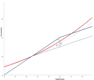
Figure 1: This figure shows how one can decom-pose the utility loss from becoming a Stackelberg follower in the drop in virtual income (A) and gains from re-optimization (B and B’). It is apparent that the second factor is greater for less productive indi-viduals.
creteness, assumeyI(wm)> yI(wf) = y¯I. Assume also that ¯yJ >yLJ(wm)> yLJ(wf)> y¯I.
BecauseyLJ(wi)>y¯Ifori=m,f, both spouses get a lower virtual income as a Stackelberg
follower than what they would obtain if filing individually. For the primary earner this drop in virtual income — represented in Figure 1 by the vertical line A – is all that takes place in terms of utility change. As for the secondary earner, it is useful to decompose her utility change in two parts. First, there is the drop in virtual income — line A. There is, however, another change which is a utility gain due to reduced labor supply by the sec-ondary earner. Note that, at the corner, the secsec-ondary earner, is working more than she
would like to for a marginal tax rate ofτ. At the budget set induced by the leader’s choice,
the secondary earner reduces her labor supply, and consumption. Because her disutility
of effort was greater than the net benefit given the marginal rate of τ, this reduction in
effort is utility increasing. This gain is represented by the segment B in Figure 1.
Figure 1 also represents the relative efficiency gains for individuals of different pro-ductivities. It is apparent that the gain is larger for the least productive individual —
B> B′. Recall, however that the drop in virtual income is larger for the secondary earner.
Whether the efficiency gain from reduced taxable income will compensate for a larger drop in virtual income, is something we cannot a priori tell. The primary earner will loose more as a Stackelberg follower than the secondary earner whenever
zyFJ(wf)−v
yF J(wf)
wf
!
>z[y¯I−∆I]−v
¯
yI
wf
,
where∆I denotes the drop in virtual income for the primary earner as a follower when
To summarize, it is usually, i.e., baring corners, the secondary earner that experiences the largest utility drop as a Stackelberg follower. It is, therefore, the secondary earner that tends to benefits most from allowing for individual filing in the sense that she obtains a larger utility gain than the primary earner. These counter-factual utility gains impact the share of surplus that each individual gains, increasing that of the secondary earner and reducing that of the primary earner, despite not changing labor supply choices.
3.1 Cournot-Nash
An alternative approach adopted in the literature is to consider a Cournot-Nash game in which individuals simultaneously choose their allocations and split taxes proportion-ately to their earnings. An individual’s share of tax duties is his or her participation in taxable income,
TCN(y
i;y−i) = yi
yi+y−iTJ
(yi+y−i). (5)
Notice that the individually effective marginal tax rate faced by an individual in the
Cournot-Nash game is not the marginal tax rate for the couple. Instead, it is a weighted average of the marginal, T′(yi +y−i), and the average,T(yi+y−i)/(yi +y−i), tax rates
faced by the couple. Precisely,
˜
τCN(yi;y−i) = (1−ωi)TJ
(yi+y−i)
yi+y−i
+ωiTJ′(yi+y−i), (6)
whereωi = yi/(yi+y−i).
In the case of progressive taxes, this means that both individuals face individually effective marginal taxes that are lower than the actual one. The logic here is that taxes over any extra dollar earned by an individual are partly transferred to the other thus reducing the tax payments at the margin (which explains how the marginal tax matters). There is, however, an extra effect that arises due to the fact that increased earnings raise the share of taxes that one is responsible for paying (which explains why average tax matters).
0 20
40 60
0 10 20 30 40 50 60 −200 0 200 400 600 800
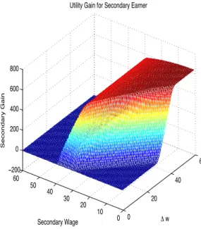
Δ w Utility Gain for Secondary Earner
Secondary Wage
Secondary Gain
Figure 2: This figure displays the difference be-tween the utility gain that the secondary and the primary earners obtain when, instead of a Stackel-berg follower under joint taxation the file individu-ally. In the figure,∆w=wm−wf.
3.2 Numeric Results
For the numeric exercises we run, we assume that the disutility of work is of the form
v(l) = l
1+γ
1+γ,
where 1/γis the elasticity of labor supply. The results we present are for the caseγ= 1,
a quadratic disutility of labor.
Our main findings for the Stackelberg counter-factual game are obtained as follows. We first calculate the utility attained by each spouse as the follower of a Stackelberg game that has the other spouse as the leader. The utility gain from having the option to file individually is the utility attained under individual taxation minus the utility attained as a Stackelberg follower. Figure 2 displays the utility gain for the secondary minus the utility gain for the primary earner. Given the structure of the bargain game we model, this counter-factual utility gain becomes the actual utility gain for the secondary earner given the couple’s allocative choices.
It is apparent that, for all couples, the difference is positive. It is, therefore, the sec-ondary earner who always benefits from the availability of a choice of schedule in our
numeric exercises. When ¯yI ≥ yI(wm) ≥ yI(wf)there is no change for either spouse in
choose the tax system. The second region illustrates this result for ¯yJ > yI(wm) +yI(wf),
and the third, foryI(wm) +yI(wf) >y¯J. The possibility of a greater gain for the primary
user whenyI(wf) =y¯Idoes not materialize in our exercises.
Allowing spouses to file individually always benefits the secondary earner in our nu-meric exercises. Our theoretical analysis in Section 3 has shown that this has to be the case provided that all choices are interior. The numeric results above generate the same
pattern at corners. In our exercise we assume thatτ < 0.5. Whenτ > 0.5, although the
leader choosesyL
J(wi)≥ y¯J, thus inducing a choice ofyFJ(wi)in the taxed region, the
op-timal choice for individual taxation might be at the kinkyI(wi) = y¯I.13 It is then possible
to easily create examples for which it is the primary that benefits most from allowing for individual filing.14
It is important to note that the utility differences are non-trivial, which shows that the non-chosen schedule plays an important role by affecting the specific allocation that is chosen in the Pareto set defined by the Nash bargain between the two spouses.
Next, we examine the consequences of adopting an alternative approach to the counter-factual game. Namely, a Cournot-Nash game with proportional tax splitting.
3.2.1 Cournot-Nash
When ¯yI ≥ yI(wm) ≥ yI(wf), it is straightforward to see that filing individually or
jointly leads to the same choices, and consequently, the same utility in the Cournot-Nash game with proportional tax sharing. This result is illustrated by the first flat region on Figure 3, which shows that the utility gain for the secondary earner is zero.
IfyI(wm)>y¯I >yI(wf), but ¯yJ > yI(wm) +yI(wf), it is always the secondary earner
who benefits from the availability of a choice between schedules. The analysis for the
same case, but when yI(wm) +yI(wf) > y¯J goes in the same direction, with identical
findings. These results are represented in Figure 3 by the second and the third region, respectively.
Finally, for the case in whichyI(wm)≥ yI(wf)> y¯I we find that allowing couples to
file individually always benefits the secondary earner. Although we have not been able to prove that this needs always happen, our numeric findings suggest that this is the most likely case. This case is represented in Figure 3 by last region, when, for a fixed secondary
13For a genericγthe equivalent condition isτ>1−2−1/γ.
14Letyτ(w
i)denote the optimal choice for an individualiwho faces a linear budget set with a marginal
0
20 40
60
0 20 40 60
0 200 400 600 800 1000
Δ w Utility Gain for Secondary Earner
Secondary Wage
Secondary Gain
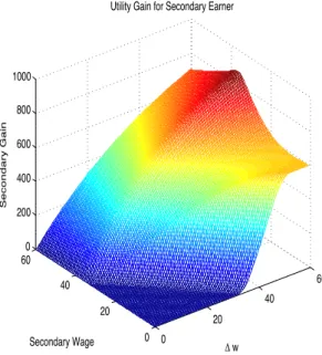
Figure 3: This figure displays the main results for the Cournot-Nash case. As we vary the productiv-ity differential between spouses the gain for the sec-ondary earner rises for any given level ofwf, pro-vided that total income is greater than the thresh-old. Utility gain is not monotonic for the secondary earner as her productivity increases for fixed pro-ductivity differences between the spouses.
earner wage, the utility gain is increasing in the productivity differential of spouses, but for a fixed productivity differences, it is decreasing in the secondary wage.
To summarize, both spouses have their utility increased in the counter-factual game when they are allowed to file individually, but the secondary earner’s utility increases more than the primary’s. I.e., the secondary earner benefits from the option to choose the tax system, corroborating that the non-chosen schedule plays an important in the Nash bargain game between the two spouses.
3.3 Break up of Marriage as the Relevant Threat
Before we close this section we address a lose end of our analysis. We discuss the possibility of ending marriage as the relevant threat. Indeed, although we have taken non-cooperation while remaining married as the relevant threat, it is not always the case that the non-cooperative equilibrium within marriage delivers more utility than breaking
up. For the Stackelberg game it suffices to assume that the leader choosesyL(w
−i)> y¯Ifor
there to be a value ofzsufficiently close to 1 to make being single better than remaining
married.
As for the Cournot-Nash case, assume that individuals have the same productivity,
efficient choice for the couple solves
max
ym,yf
z
ym+yf −2T
y
m+yf
2
−vym w −v y f w ,
which has as first order conditions
z
1−T′
y(wm) +y(w
f)
2
=v′
y(wi)
wi
1
wi
. (7)
Becausewm =wf (7) becomes
zw
1−T′(y(w))
=v′(y(w)/w), (8)
whereT′(y(w)) = τ. That is, the efficient solution is exactly the same that obtains under
individual taxation. Note that whenz=1, (8) is exactly the breaking up solution.
The Cournot-Nash allocation, however, has
zw
1−τ
1−1
4 ¯ yJ
yCN(w)
=v′
yCN(w)
w
,
which is inefficient.
For z sufficiently close to 1 the inefficiency dominates the returns of scale and being
single is better than remaining married. It is important to note that whenever this hap-pens, the fact that the tax system allows for couples to choose benefit the primary earner. The reason is that gains from being able to file individually (in the non-cooperative game)
instead of breaking up marriage are higher for the primary earner.15
4
An Alternative Tax System
The tax system we studied in Section 3 essentially treats a couple’s average income as if it were the income of a single individual. This, combined with the convexity of the budget set means that it is never optimal for a couple to file individually. In this section, in contrast, we consider a tax system for which this need not be the case.
The tax system we study now is as follows. If spouses file individually, total taxes as a
15Indeed,
d
dzmax
n
z[y−T(y)]−vy
w
o
function of taxable income,y, are
TI(y) =
(
0 fory≤y¯I,
τ[y−y¯I] fory>y¯I,
whereτ, ¯yI >0. If, instead, the couple files jointly, then
TJ(ym+yf) =
(
−B forym+yf ≤y¯J,
−B+τ[ym+yf −y¯J] forym+yf >y¯J,
where ¯yJ = y¯I =y, and¯ B>0.
In other words, this tax system treats the income generated by couples and that gen-erated by single persons (or married persons filing individually) identically, except for the fact that married couples are entitled to a positive transfer (a demogrant or a deduc-tion). Indeed, many countries provide all types of deductions and ’subsistence transfers’ for families despite not necessarily offering special tax treatment for couples. Of course, in some places we see a mix of the two types of treatments, and we hope that our analysis will shed light on the probable consequences for the different systems.
As already mentioned, the only difference between the joint and the individual sched-ules is the demogrant, present for the former and absent for the latter. Under our
as-sumption about tax sharing in the Stackelberg counter-factual game, the demograntBis
all taken by the leader. This deduction increases the leader’s utility but has no effect on his or her choice:yLJ(wi) =yI(wi)fori= f,m. Note, however, that the leader’s utility is
not an object of our interest since we want to analyze the utility each spouse attains as a
follower. Yet,Bdoes play a role in our analysis, since its value is critical in determining the
regions for which either system dominates.
The efficient choice for couples need not to be to file jointly under this alternative tax system. The ’envelope schedule’ could, therefore, be a more complicated object than what
we were previously considering. In particular, if B ≥ τy, then filing jointly is always¯
better for a couple, whereas ifB<τy, this is not always case.¯
Let us start withB≥τy¯in which case the couple can never do better by filing
individ-ually: TJ(.)is itself the envelope of the whole tax system. Note, however, that TI(.)still
plays a role, which is different from the one in the previous tax system. The convexity of the budget set guarantees thatBF(y)⊆ BF(y′)⇔ y ≥ y′, just as in the tax system of Sec-tion 3. Yet, contrary to what happened there, a bundle chosen by the primary earner
un-der individual filing may cease to be available in the Stackelberg game even ifyI(wf)≤y.¯
0
10 20 30
0 10 20 30 −20 −15 −10 −5 0 5 10 15 20
Δ w Utility Gain for Secondary Earner
Secondary Wage
Secondary Gain
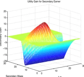
Figure 4: This graph displays the relative gain for the secondary earner for the case in whichB≥τy¯.
The negative regions of the graph indicates cou-ples, i.e., pairs (wf,wm) for which the secondary earner is hurt by the option to file individually.
choicesin the Stackelberg game, even when choices are in the interior of each bracket.16
This will, in general, preclude a general statement about who benefits most from filing individually.
When yI(wf) +yI(wm) ≤ y, the move from individual tax schedule to the joint one¯
does not change anything since both spouses make the same choices and have the same utility.
The analysis is not so straightforward when yI(wi) ≤ y¯ for i = f,m, but yI(wf) +
yI(wm)> y. As¯ yI(wi)> y¯−yLJ(w−i), the chosen bundles are no longer feasible for both
spouses in the Stackelberg game. If both spouses choose at the kink as Stackelberg
follow-ers, then their consumptions are reduced by the exact same value.17It is possible to show
that the utility drop for the secondary earner is greater.18In fact, the result is valid even if
we allow individuals not to choose at the kink, even though, the drop in consumption is no longer identical for the two individuals. As a consequence, the secondary earner is the one who benefits most from the choice of the tax filing.
When yI(wf) < y¯ < yI(wm), the primary earner utility varies only due to a drop in
consumption ofτyI(wf). As for the secondary earner, her utility changes due to both a
16Recall thatyL
J(wi)andyJF(wi)are the taxable incomes of a person of productivitywias a leader and a follower in the Stackleberg game, respectively, andBF(yL(w−i))is his or her residual budget set as in 4. In
the benchmark example, although we could observe simultaneous changes in consumption, giveny, for both
individuals to change their choices, we needed choices to be at the kink of the tax schedule.
17Ifiremains at the kink,y
I(wi)−yFJ(wi) = yI(wi)− h
¯
y−yLJ(w−i) i
=yI(wi) +yLJ(w−i)−y¯ =yI(wi) +
yI(w−i)−y¯=yI(w−i)− h
¯
y−yL
J(wi) i
=yI(w−i)−yFJ(w−i).
18The rationale is a bit involved since it requires comparing the slopes of spousesat different bundles. A
drop in consumption and a drop in taxable income. Assume that the secondary earner
does not re-optimize, i.e., she choosesyI(wf)at the new budget set. Her utility decreases
by total taxes paid, τyI(wf) which is exactly the same drop in utility that the primary
earner experiences. Because the secondary earner re-optimizes, she is the one that expe-riences the smallest drop in utility. It is therefore the primary who benefits most from having the option to file individually. Finally, whenyI(wi)>y¯fori= f,m, both spouses
make the same choices and lose the same utility. So, no one benefits from the choice of tax filing.
Results for this case are in Figure 4. Even though the budget sets are still convex, mean-ing that the budget set of the secondary earner as a Stackelberg follower is weakly smaller
than that of the primary earner, for a large region of thewf ×wm space it is the primary
that benefits from having the option to file individually, as theoretically predicted.
When B < τy, the individual tax schedule is not dominated by the joint schedule.¯
Parts of the envelope coincide with the individual tax schedule while others, with the joint tax schedule. When one of the spouses earns very little it may be better to file jointly,
whereas for large values ofym+yf it will be better to file individually. This lack of
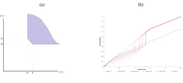
dom-inance may induce non-convexities on budget sets. Figure 5 illustrates the budget sets defined by this alternative tax structure. Non-convexity and the consequent discontinuity of choices are apparent.
(a) (b)
0 0,2 0,4 0,6 0,8 1 1,2 1,4 1,6 1,8 2
0 0,5 1 1,5 2 2,5 y(w-i) = 0 y(w-i) = B/t = 1 y(w-i) = 1.15 y(w-i) = 1.25 y(w-i) = 1.35 y(w-i) = 1.5
Once again, we break the analysis in different cases.
IfyI(wf) +yI(wm) ≤ y, the couple prefers to file jointly given the tax deduction. In¯
this sense, there is no change in moving from separate to joint filing since both spouses make the same choices under either system.
Things become more interesting whenyI(wi)≤y¯fori= f,m, butyI(wf) +yI(wm)>
¯
y. IfyI(wf) +yI(wm)≤ B/τ+y, the couple prefers to file jointly. Otherwise, they prefer¯
to file individually.
In the former sub-case, i.e.,yI(wf) +yI(wm)≤ B/τ+y, the analysis is identical to the¯
one presented for the analogous situation withB> τy, and it is the the secondary earner¯
who benefits from the availability of a choice of the tax schedule.
The second sub-case,yI(wi) +yI(w−i) > B/τ+y, leads to the non-convexity of the¯
follower’s budget set, inducing discontinuity in his or her choices with respect to the leader’s. Non-convexity arises due to the fact that the envelope results from a
maximiza-tion of two schedules, which yields regions of theym×yf space where it is efficient to file
jointly and regions where it is optimal to file individually. When it is efficient for the cou-ple to file individually, moving from separate filing to the envelope does not benefit any spouse. Note that this sub-case is only possible if the leader choosesyLJ(wi)∈(B/τ, ¯y].
Another interesting case arises whenyI(wf) < y¯ < yI(wm). Now, ifyI(wf) < B/τ,
spouses prefer joint taxation. Quasi-linearity then implies that there is no impact on the
primary earner’s labor supply, yFJ(wm) = yI(wm), since he faces the same marginal tax
rate in either situation. However, as the exemption is ¯y−yLJ(wf), his budget set reduces
and he losesτyI(wf) utility when moving from separate to joint filing. The secondary
earner, on the other hand, faces a higher marginal tax rate leading to yFJ(wf) < yI(wf).
Note, however, that similarly to the analogous situation when B > τy, the secondary¯
earner’s utility changes due to a drop in consumption and taxable income, and she is the one that experiences the smallest drop on utility since she re-optimizes.
If, however,yI(wf)> B/τ, choices take place in the region where individual taxation
is best and there is no change in equilibrium since both spouses make the same choices. The last case is whenyI(wi)>y¯fori= f,m. The couple will always prefer individual
filing. Both spouses, therefore, choose above the exemption ¯y, meaning that they will
make the same choices under either filing choice. Hence, there is no change in utility. Our numeric exercises illustrate our theoretical findings. We observe a large region in which the secondary earner is hurt by the option to file individually — Figure 6. Note that this is not a consequence of non-convexity, since this result was present in the case B>τy.¯
discontinu-0 5 10 15 20 25 30 0 10 20 30 −200 −150 −100 −50 0 50 100
Δ w Utility Gain for Secondary Earner
Secondary Wage
Secondary Gain
Figure 6: This figure displays the difference in util-ity gains for secondary and primary earners as fol-lowers of a Stackelberg game from moving to indi-vidual taxation. Negative values indicates that pri-mary earners benefit most from having the option to file individually.
0 10 20 30
75 80 85 90 95 100 Wage Difference Labor S uppl y
Secondary Wage = 7
0 10 20 30
60 70 80 90 100 Wage Difference Ut ili ty
Secondary Wage = 7
0 10 20 30
300 350 400 450 500 550 600 650 Wage Difference Labor S uppl y
Secondary Wage = 14.5
0 10 20 30
300 320 340 360 380 400 420 440 Wage Difference Ut ili ty
Secondary Wage = 14.5
0 10 20 30
600 700 800 900 1000 1100 Wage Difference Labor S uppl y
Secondary Wage = 20
0 10 20 30
720 740 760 780 800 Wage Difference Ut ili ty
Secondary Wage = 20
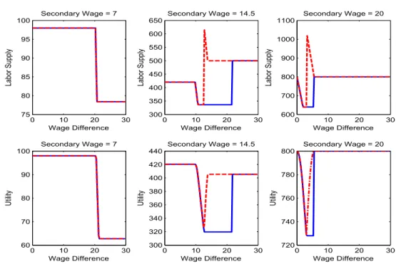
Figure 7: These figures show how labor supply (panels in the top) and the utility (panels in the bottom) of
a follower, characterized by its productivitywias a function of the leader’s labor supply choice. Each pair
ity in the equilibrium utilities that arise in the Stackelberg game. Although discontinuity in choice is immediate from the non-convexity of the budget set, discontinuity of utility is more subtle. Key to understanding this is to realize that the Stackelberg leader may be willing to distort his or her choice to induce the follower not to go to the region of the envelope that corresponds to individual taxation. This will be done up to the point where the cost of deviating from his or her preferred choice just equates the gain from remaining
in the joint schedule. There will be a threshold valuew−iabove which the leader no longer
distorts his or her choice thus jumping straight to his or her optimum. This generates a discontinuous change in the follower’s budget set that induces the discontinuity in utility.
5
Conclusion
We adopt Lundberg and Pollak’s (1993) separate spheres of bargain approach to a couple’s decision making process to analyze the consequences of tax filing options for each spouses outcomes.
We model a Stackelberg counter-factual game in which one of the spouses acting as the leader earns his or her taxable income, pays taxes and leaves the residual budget set
for the follower. We use each spouse’s utility attainedas a followeras the threat point of
the Nash bargaining game that establishes how the surplus of marriage is split between spouses.
Our benchmark tax system resembles that of the US in that joint taxation amounts to treating a couples’ average earnings as if it were the earnings of an individual. Under this benchmark tax system it is always the secondary earner that benefits from the option of filing individually. When we consider an alternative system that simply includes a de-ductible for the couple but otherwise treats total income as if it were that of a single agent,
the results are changed. For many couples, identified in this paper as a pair(wf,wm), it
is the primary earner who benefits from the option of filing individually. In all cases, the results are quantitatively relevant.
With regards to public policy recommendation, our results show that allowing couples to choose has important distributional consequences within households. It also shows that whoever will benefit crucially depends on the details of the tax system.
References
Alesina, Alberto, Andrea Ichino, and Loukas Karabarbounis, “Gender Based Taxation
1–40.
Becker, Gary S., “A Theory of Marriage (Part II),”Journal of Political Economy, 1974, 82,
511–526.
,A Treatsie on the Family, 2nd ed., Cambridge, MA: Harvard University Press, 1991.
Chiappori, Pierre-André, “Nash-Bargained Household Decisions,”International Economic
Review, 1988,32, 791–796.
and François Bourguignon, “Collective Models of Fousehold Behavior: An
Introduc-tion,”European Economic Review, 1992,36, 355–365.
Feenberg, Daniel R. and Harvey S. Rosen, “Recent Developments in The Marriage Tax,”
Technical Report, NBER Working Paper 1994.
Lundberg, Shelly and Robert A. Pollak, “Separate Spheres Bargaining and the Marriage
Market,”Journal of Political Economy, 1993,101(6), 988–1010.
Manser, Marilyn and Murray Brown, “Marriage and Household Decision Making: a
Bargaining Analysis,”International Economic Review, 1980,21(1), 31–44.
McElroy, Marjorie B. and Mary Jane Horney, “Nash-Bargained Decisions: Towards a
Generalization of the Theory of Demand,” International Economic Review, 1981,22 (2),
333–349.
Pollak, Robert A., “Family Bargaining and Taxes: A Prolegomenon to the Analysis of
Joint Taxation,”CESifo Economic Studies, 2011,57(2), 216–244.
Samuelson, Paul, “Social Indifference Curves,” Quarterly Journal of Economics, 1956, 70,
1–22.
Ulph, David, “A General Non-cooperative Nash Model of Household Consumption
Be-havior,” 1988. Working Paper 88-205 - Department of Economics, University of Bristol.
Wooley, Frances, “A Non-cooperative model of family decision making,” 1988. TIDI
A
The Cournot-Nash Game
LetyI(w)denote the taxable income of someone who is married, is filing individually
and whose skill isw.19
In most of what follows we shall use the expression ’the’ Nash equilibrium, even though there might be multiple equilibria at the kink of the couple’s budget set. We dis-cuss this case at the end of this section and explain how we deal with it in practice in our numeric exercises. In this case, the Nash equilibrium should be understood a selection from the set of Nash equilibria. We shall also focus on pure strategy Nash-equilibria. As we shall make clear, such an equilibrium may not exist when we consider in Section 4 a non-convex budget set.
We start our analysis by noting that filing individually or jointly leads to the same choices and utility if ¯yI ≥yI(wm)≥yI(wf).
Let us, then, assume that yI(wm) > y¯I > yI(wf), but ¯yJ > yI(wm) +yI(wf). We
would like to construct the counter-factual choices of this couple if they decided to file
jointly but act non-cooperatively. Holding yf, the consequence of moving to joint filing
for individualmis to reduce his marginal tax rate and to increase his labor supply. Let
yCN(w
i)be the equilibrium choice of an individual with productivitywifor the
Cournot-Nash joint taxation game. Ifym does not increase very much, then there is no impact on
f’s labor supply and utility. If, on the other hand,mincreases enough his labor supply,
we may haveyCN(w
m) +yCN(wf)≥y¯Jin which case (6) becomes
˜
τCN(yi;y−i) =τ
1−ω−i
¯ yJ
yi+y−i
.
Because the effective marginal tax rate for f increases,yI(wf)≥yNC(wf).
What happens to the utility ofm and f? Recall that total taxes paid by each spouse
under joint filing is
TCN(yi;y−i) =τ
yi− yi
yi+y−i
¯ yJ
ifyCN(wm) +yCN(wf)≥y¯Jand 0, otherwise.
Since ¯yI >yI(wf), we have thatTCN(ym;yf)< TI(ym)for allym > y¯I.20 As taxes are
always lower for the primary earner, given that he can transfer part of his tax payments to the secondary earner, his budget set is larger under Cournot-Nash game. The opposite occurs for the secondary earner which confirms the idea that the option to allow couples
19Because we treat individuals symmetrically we need not index the functiony
I(.)with the individual’s type.
1,8 2 2,2 2,4 2,6 2,8 3
C
o
n
s
u
m
p
ti
o
n
1 1,2 1,4 1,6
1 1,5 2 2,5 3 3,5 4
Taxable Income
Individual y(wf)=0 y(wf)=0.25 y(wf)=0.50 y(wf)=0.75 y(wf)=1
Figure 8: The lower curve (continuous in blue) de-fines the budget set for the primary earner under individual filing. The upper, continuous curve in red is the Cournot-Nash budget set for the primary earner wheny(wf) =0. The following dotted lines are his budget sets fory(wf) =0.25,y(wf) =0.5,
y(wf) =0.75 andy(wf) =1.
to file individually favors her in this situation.
A similar analysis applies ifyI(wm) > y¯I > yI(wf), andyI(wm) +yI(wf) > y¯J. With
joint taxation, the ’effective’ marginal tax rate faced by the primary earner decreases,
while that of the secondary earner will not decrease and may in fact increase ifyCN(wm) +
yCN(wf) ≥ y¯J. Either way, it is clear again that allowing individuals to file individually
will not hurt and will sometimes help the secondary earner.
Finally, assume thatyI(wm)≥yI(wf)>y¯I. In this case, the Cournot-Nash equilibrium
of the joint taxation case entails necessarily a higher taxable income by both individuals. With regards to utility, things get a little more complicated in this case. Let us start our analysis by considering the secondary earner.
As long asyf ≤ym, we haveTCN(yf;ym)>TI(yf). This means that the set of feasible
choices that will arisein equilibriumfor the secondary earner is a subset of what is possible
under individual filing. The secondary earner, therefore, always loses by not having the option to file individually when a Cournot-Nash game is played.
Things are somewhat more subtle for the primary earner. The feasible sets are, once
again, defined byTCN(y
m;yf), withTCN(;yf)≤ TI()wheneverym >yf. We know that,
in equilibrium, this must be the case. Therefore, the observed choice ofmwill be such that
total taxes paid will not exceed whatmwould have paid if the sameywere chosen, under
TI, i.e., TCN(yCN(wm);yCN(wf)) ≤ TI(yCN(wm)). This does not allow us to conclude,
however, thatm’s utility is higher. The budget set ’available’ to a primary earner under
joint taxation is no larger than that which is available under individual taxation.21
It is apparent that, provided that the taxable incomes — or, more fundamentally,
pro-21For example, ify
ductivity of the two individuals — are not too close, the primary earner’s utilitycannot increase when one moves to joint taxation. Although we are not able to rule out the possi-bility that, when productivities are close, the utility of the secondary earner increases more than that of a primary earner, we were not able to numerically find counter-examples that generate this result.
We have so far disregarded the possibility of multiple equilibria. As it turns, the exis-tence of a kink in the budget set creates the possibility of multiple equilibria; a continuum
of combinations of taxable incomesym andyf such thatym+yf = y¯J being equilibria of
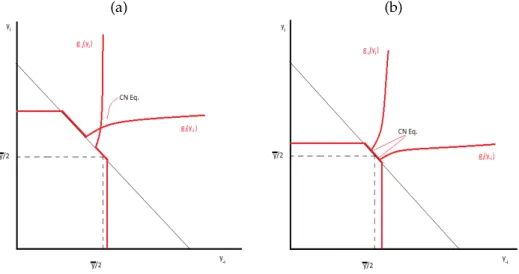
the Cournot-Nash game played by the couple. The left side of Figure 9, Fig. A, displays a situation with a unique equilibrium at which both individuals pay taxes, while the figure at the right, Fig. B, displays a situation with multiple equilibria taking place at the kink of the couple’s budget set.
(a) (b)
Figure 9: These figures illustrate a situation with a unique equilibrium at which the couple is taxed — panel (a), and a situation with multiple equilibria — panel (b) — in which the couple stays at the kink of its budget set,yCN(wm) +yCN(wm) =y¯J.